Velocity-Free Formation Control and Collision Avoidance for UUVs via RBF: A High-Gain Approach

Abstract

This paper designs an adaptive formation control system for unmanned underwater vehicles (UUVs) in the presence of unmeasurable states and environmental disturbance. To solve the problem of unmeasurable UUV states, a filtered high-gain observer (FHGO) is employed to estimate the states, despite measurement noise. Then, an adaptive control scheme is designed to achieve UUV formation collision avoidance. The radial basis function (RBF) is used to estimate the unknown disturbance. The stability of UUV formation with collision avoidance is proven by using the Lyapunov theorem. Numerical simulation is carried out to demonstrate that the proposed filtered high-gain observer is successful in estimating the states of UUVs. The control law can keep the UUV formation from collision with good performance.

1. Introduction

Due to its high efficiency and wide searching area, formation control for multiple agents has become a hot topic. In the research process, there are a lot of challenges to address, such as nonlinearity in parameters, communication constraints and dynamic environmental disturbance. Various methods have been proposed for the formation control of autonomous underwater vehicle (AUV) groups in a decentralized manner, which is also known as high-level control, examples of which include artificial potential field or methods based on agreement protocol such as leader–follower, virtual structure and behavioral approaches [1,2,3]. In [4], an adaptive neural network formation controller was developed for multiple AUVs with unknown model coupling terms and unknown disturbances. A neuroadaptive sliding mode formation controller was proposed for multiple AUVs with environmental disturbances [5]. Gao proposed a fixed-time sliding control scheme with a disturbance observer to solve the compound disturbance, including both external environment disturbance and parameter uncertainties [6]. Based on the minimal learning parameter algorithm, Lu proposed a robust adaptive formation controller to achieve the formation control of multiple underactuated surface vessels (USVs) [7]. Due to the complicated underwater situation, the research progress of UUV formation is relatively slow, but research on unmanned aerial vehicle (UAV) formations, autonomous ground vehicles and multiagents is advancing. In [8], an adaptive neural network control scheme was investigated to address the formation control problem of multi-USVs with data dropout and time delays [9].

Based on the approximation of a partial differential equation modeling the nonlinear steady state, the characterization of the low-pass filtering to high-frequency measurement noise of high-gain observers has been proved in [10]. High-gain observers are a good choice for dealing with the influence of noise. It is fundamental to recall that the performance of a high-gain observer in the presence of colored measurement noise is mainly characterized by its dominant linear behavior, if the frequency of the noise is large enough, as shown in [10,11]. In [12], a fixed-time state observer was designed to estimate velocity state, and a fuzzy adaptive sliding mode control law was proposed to achieve trajectory tracking. In the absence of high-frequency measurement noise, high-gain observers can simultaneously reject modeling uncertainty and quickly reconstruct the system states. In fact, to achieve the objectives of fast state estimation, the chosen observer gain must be sufficiently high. However, measurement noise introduces an upper limit for the gain when good performance is considered. Prasov applied a nonlinear gain approach to overcome the trade-off between fast state reconstruction and measurement noise attenuation [13]. The idea behind the inclusion of dead-zone nonlinearity in a high-gain observer is to achieve a large gain when the system is still in the transient phase. Hence, state estimations can approach the true state values significantly fast. When the estimation error is sufficiently small, the observer gain is small. Thus, the measurement noise can be attenuated. The second solution is a modified high-gain observer, which applies a low-pass filter to standard high-gain observers to reduce the effect of measurement noise [11].

In [14], an adaptive neural tracking control scheme was designed to solve a class of uncertain switched stochastic nonlinear pure-feedback systems, and radial basis function (RBF) neural networks were used to approximate the unknown nonlinear functions. The RBFNN was also adopted in the uncertain switched nonlinear systems to estimate nonstrict-feedback forms, and the error caused by the RBFNN was compensated [15]. The uncertain switched nonstrict-feedback nonlinear systems used the RBFNN to cope with uncertain nonlinear parts [16].

Research on the collision avoidance strategy of multiagents has been deepened. In [17,18], types of potential functions were designed to achieve connectivity preservation and collision avoidance, and the Lyapunov function was used for stability analysis. For multiagent systems, the virtual potential force of the artificial potential field (APF) was treated as an external disturbance, which proved to be robust based on H ∞ analysis in [19]. Bong investigated a USV formation system that suffered from heterogeneous limited communication ranges and designed a novel nonlinear transformed formation error for achieving initial connectivity preservation and collision avoidance [20]. In [21], a distributed control strategy was presented for a multiagent system to reach the target plane with a predesigned orientation, circulate around the target with a prescribed radius, and avoid collisions among multiagents. He and Wang proposed a formation control method with collision avoidance for actuated multi-USVs to address parametric and nonparametric uncertainties and external disturbances by imposing proper prescribed performance [22]. By integrating the gradient of a repulsive APF with a fast terminal sliding mode surface, a novel sliding mode surface-like variable was improved for a position control scheme of USV formation [23].

Motivated by the above observations, this paper presents an adaptive neural network control scheme for UUV formation with unmeasurable states. The specific contributions of this paper can be summarized as follows:

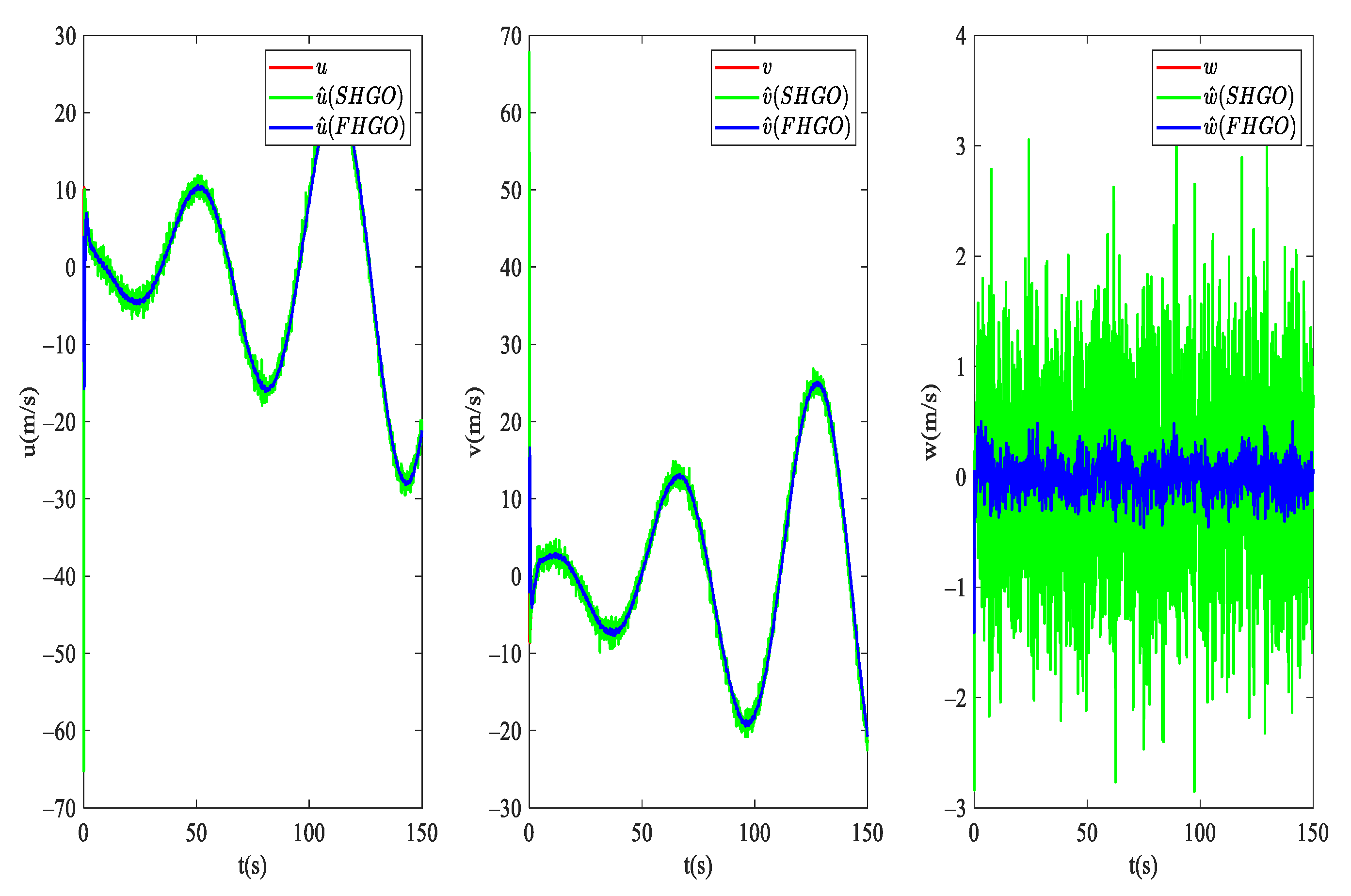
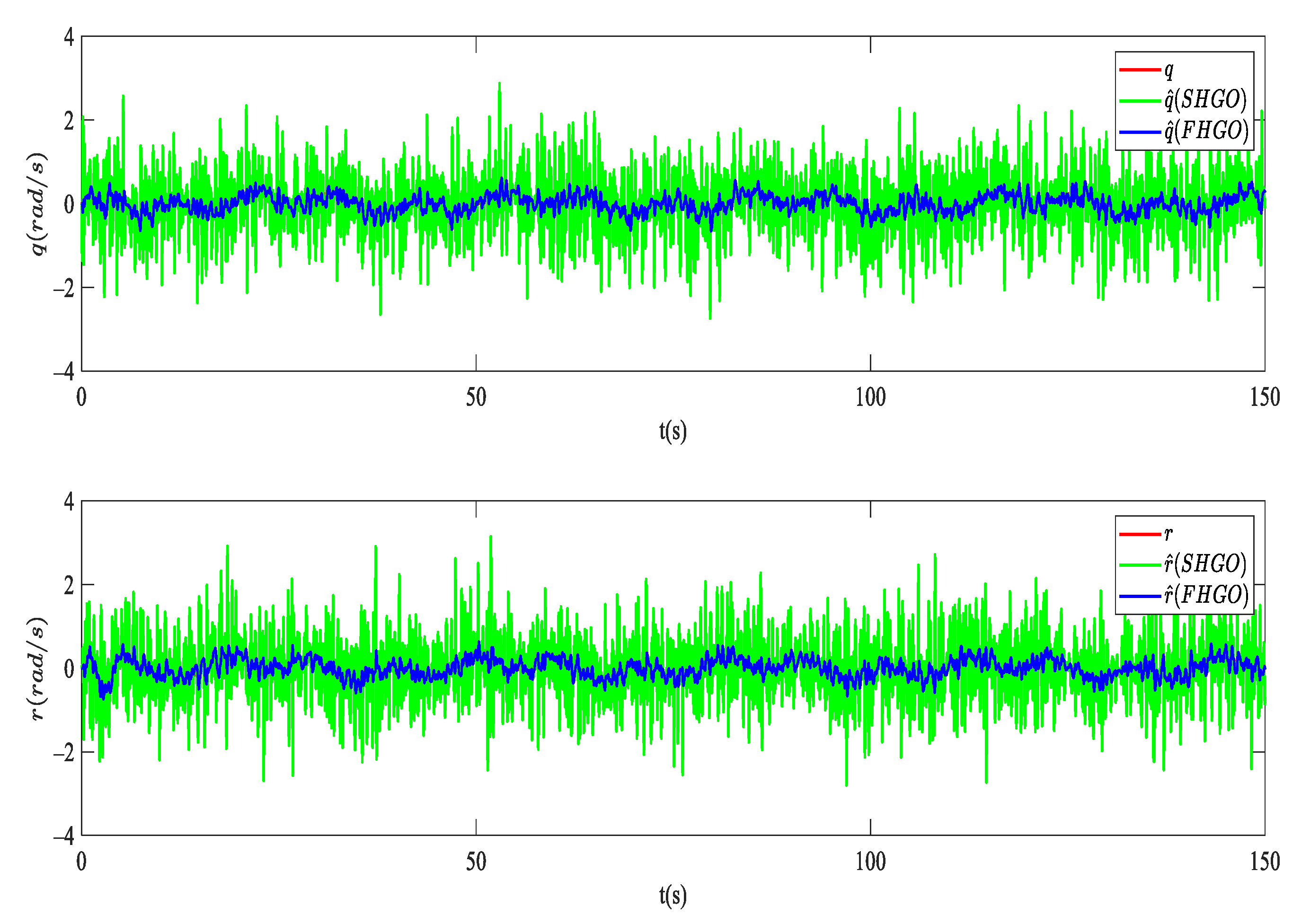
• An FHGO is designed to exactly estimate the states of UUVs to satisfy the so-called observer matching condition. Differently from [10], the input-to-state stability property of the estimation error is still preserved in the presence of measurement noise;
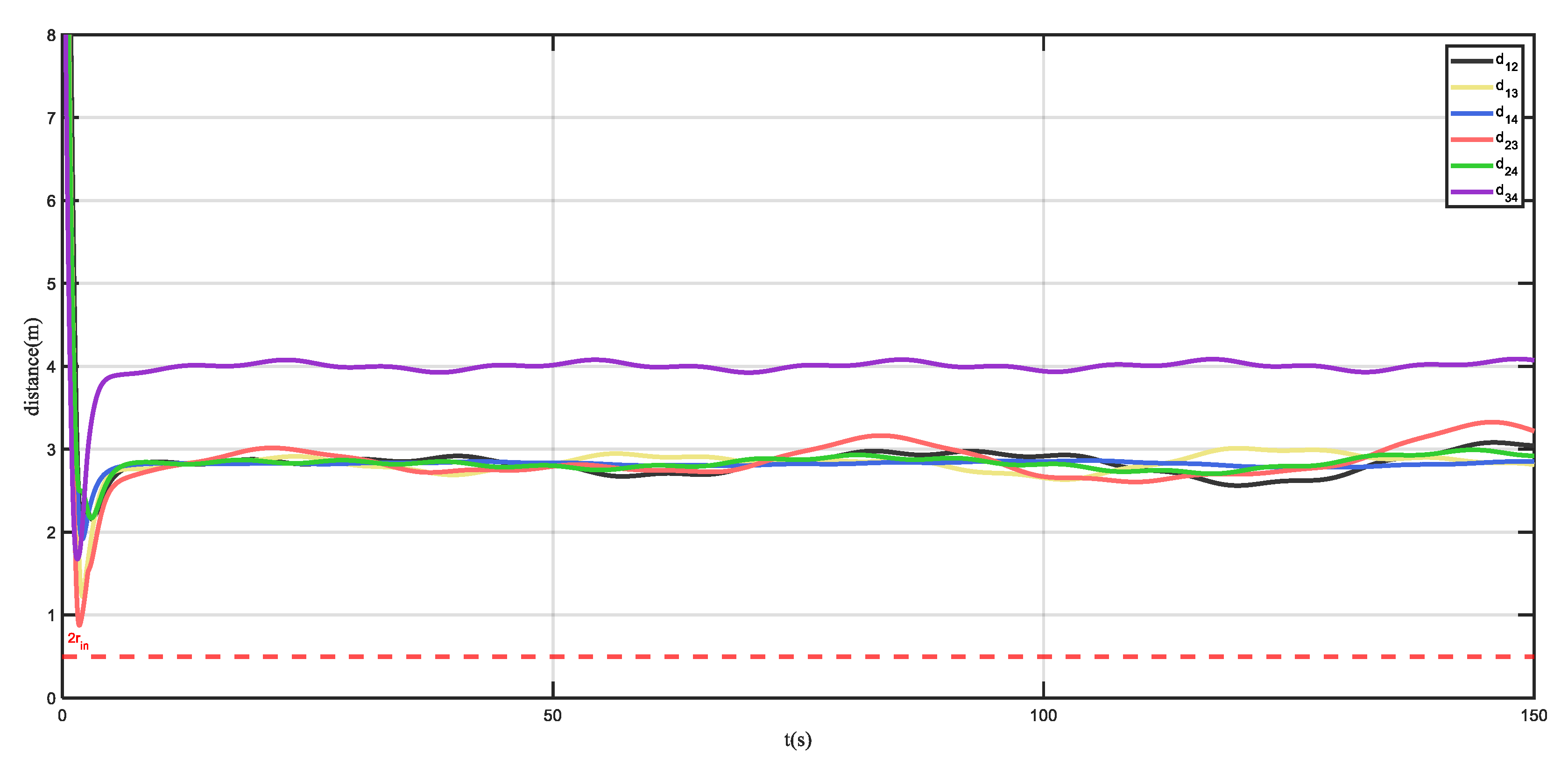
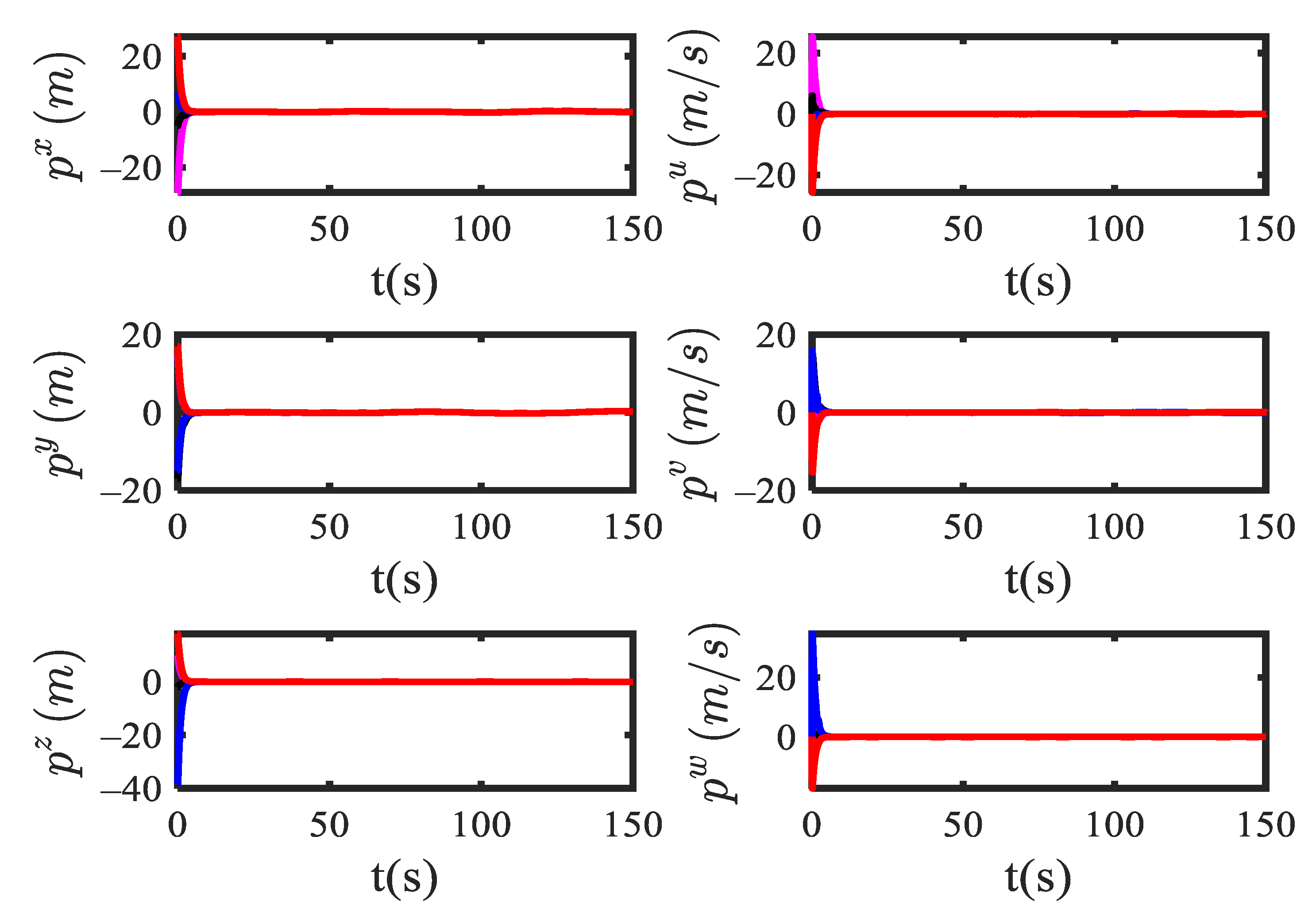
• An adaptive neural network formation control scheme is designed for UUV formation with collision avoidance under unknown disturbance. The RBF neural network is used to estimate the unknown disturbance. Studies on collision avoidance for multi-UUV formation are mostly on the 3-DOF model in the horizontal plane. The state feedback linearization method is used to transfer the nonlinear and coupling mathematical model of UUVs into a second-order system model in 5-DOF. The artificial potential field theory is applied to cope with collision avoidance among the UUVs. The form of the potential function is much simpler;
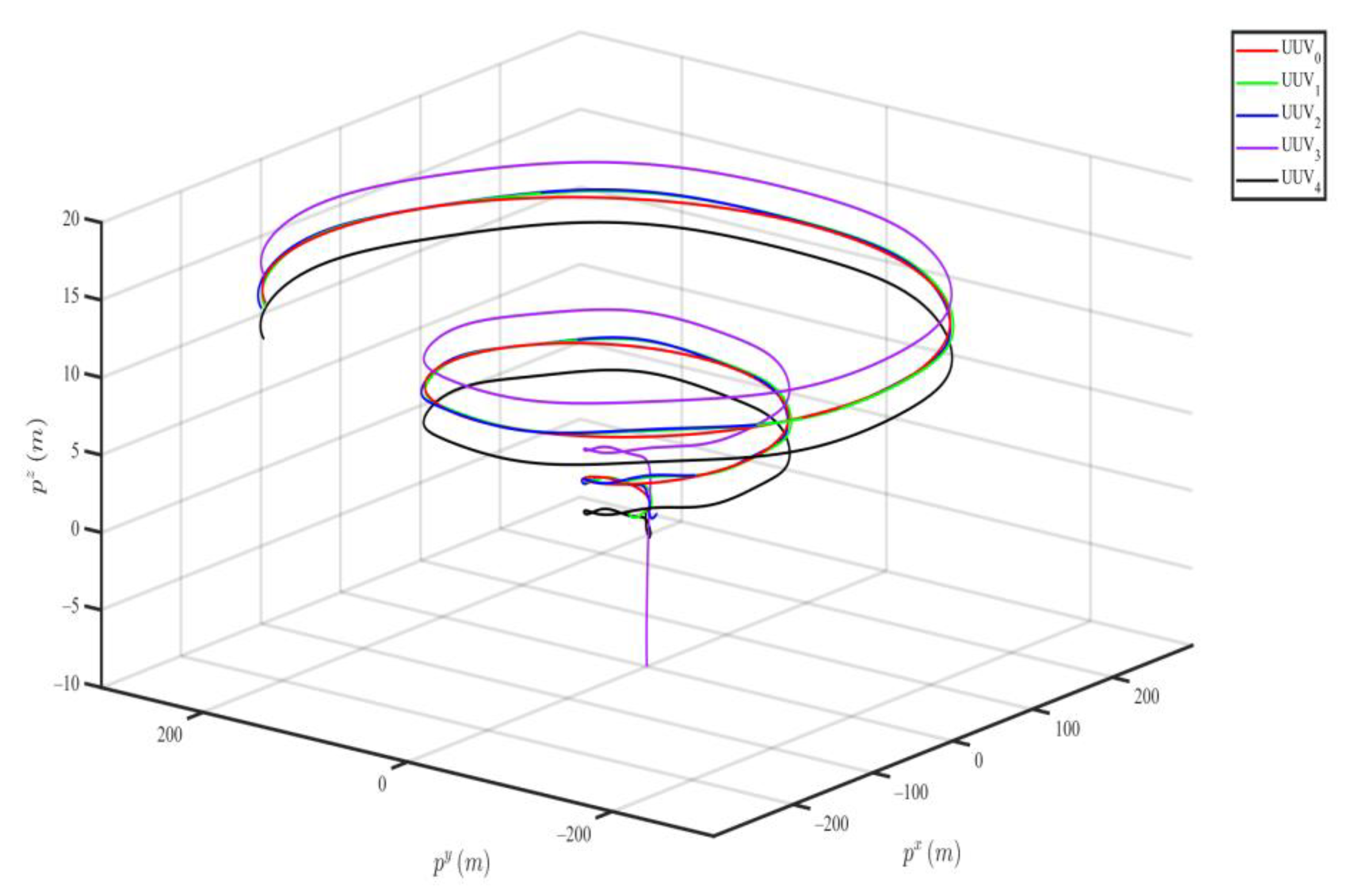
• Based on the Lyapunov theory, the stability of the formation system is proven. The proposed controller is valid and performs well, which can be found in the 3-D simulation figures.

2. Preliminaries and Problem Formulation

2.1. Graph Theory

Considering a multi-UUV system consisting of $n$ vehicles, we use graph theory to model the information exchange among UUVs. Let the graph $G=(N,E,A)$ be an undirected graph, which consists of a node set $N=\left\{n_1,n_2,\cdot \cdot \cdot ,n_n\right\}$, an edge set $E\subseteq N\times N$ and the adjacency matrix $A=\left[a_{ij}\right]\in R^{n\times n}$. The element $a_{ij}=1$ denotes that the node $i$ can receive information from the node $j$; otherwise $a_{ij}=0$, and for all, $i$, $a_{ii}=0$. Moreover, $G$ is undirected if $a_{ij}=a_{ji}=1$. The collection of connected neighbors of $n_i$ is denoted as $N_i=\left\{n_j\in N:(n_j,n_i)\in E\right\}$. The in-degree matrix $B=diag\{b_1,b_2,\cdots b_n\}\in R^{n\times n}$ is a diagonal matrix, where $b_i={\displaystyle \sum _{j=1}^n{a}_{ij},i=1,2,\dots ,n}$ is the in-degree of node $n_i$. Then, the Laplacian matrix $L=\left[l_{ij}\right]\in R^{n\times n}$ is defined as $L=B-A\in R^{n\times n}$. Define $\vartheta =diag\{{\theta }_1,{\theta }_2,\dots ,{\theta }_n\}$, which is the communication weight matrix between $UU{V}_i$ and the virtual leader, where ${\theta }_i=1$ means that $UU{V}_i$ can receive the information from the virtual leader, and ${\theta }_i=0$ means otherwise. Then, we obtain the matrix $\overline{L}=L+\vartheta$, and the eigenvalues of $\overline{L}$ are positive.

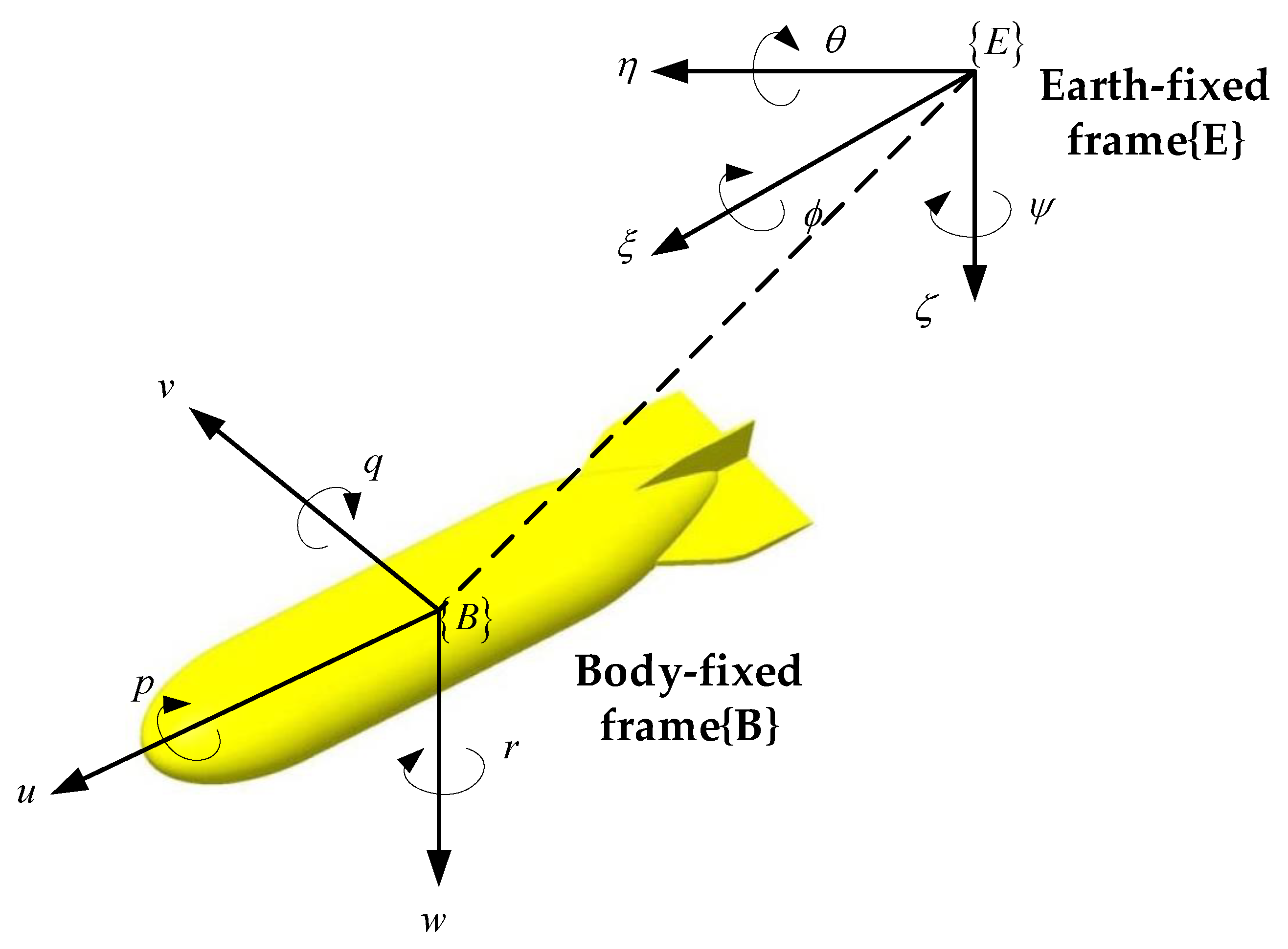
2.2. Feedback Linearization of UUV Model

The kinematic and dynamic model of a UUV are described in two coordinate frames, which are the Earth-fixed frame {E} and the body-fixed frame {B}, as shown in Figure 1.

According to the structure of the UUV studied in engineering applications, there is no thruster to control the angular velocity in roll. Meanwhile, the rolling has little influence on the translational motion, so the roll speed can be ignored. Then, the kinematic and dynamic equations of UUVs can be described as [24]:

$$\begin{array}{c}{\dot{p}}_0=J(p_0)v_0\\ M_0{\dot{v}}_0={\tau }_0+{\omega }_0-D\left(v_0\right)v_0-\mathrm{C}\left(v_0\right)+\overline{\Delta }(v_0)\\ y_s=p_0+{\omega }_n\end{array}$$

(1)

where $p_0={[p_0^x,p_0^y,p_0^z,p_0^{\theta },p_0^{\psi }]}^T$ denotes the position and the attitude angle of the UUV in the Earth-fixed frame. $v_0={[v_0^u,v_0^v,v_0^w,v_0^q,v_0^r]}^T$ is the velocity vector of the UUV in the body-fixed frame. ${\omega }_0\in {ℝ}^5$ is an unknown time-varying disturbance due to currents and waves. ${\tau }_0\in {ℝ}^5$ is the control input acting on the UUV in the body-fixed frame. $\overline{\Delta }(v)$ represents the parameter uncertainty. ${\omega }_n$ denotes the measurement noise. Additionally, $J(p_0)$ is the transformation matrix. $M_0$, $D(v_0)$ and $C(v_0)$ denote the inertia matrix, damping matrix and the matrix of Coriolis and centrifugal terms, respectively.

The mathematical model of UUV is nonlinear and has strong coupling. To solve the problem, the feedback linearization method is adopted to simplify the UUV model. The standard double integrator dynamic model can be described as:

$$\begin{array}{c}\dot{p}=v,\\ \dot{v}=\tau ,\\ p\in {ℝ}^5,v\in {ℝ}^5\end{array}$$

(2)

The specific linearization process can be obtained from [25]. In (3), the external disturbances are not considered. Since the disturbance is unknown and nonlinear, no matter how the conversion is performed in the linearization process, the final form of disturbance is still unknown and nonlinear. Then, a modified linearization model is proposed in this paper as:

$$\begin{array}{c}{\dot{p}}_i=v_i\\ {\dot{v}}_i={\tau }_i+\omega \end{array}$$

(3)

where $p_i={[p_i^x,p_i^y,p_i^z,p_i^{\theta },p_i^{\psi }]}^T\in {ℝ}^5$ and $v_i={[v_i^u,v_i^v,v_i^w,v_i^q,v_i^r]}^T\in {ℝ}^5$ are the position and velocity of the $UU{V}_i$ in UUV formation with $i=1,2,\dots ,n.$ ${\tau }_i\in {ℝ}^5$ is the control input of $UU{V}_i$. $\omega \in {ℝ}^5$ is an unknown time-varying disturbance.

Due to the complexity of the underwater environment, if faults occur to the leader in the leader–follower method, the mission of UUV formation will not be able to be completed. To enhance the fault tolerance ability of the formation control, a virtual leader is introduced and defined as:

$$\begin{array}{c}{\dot{p}}_l=v_l\\ {\dot{v}}_l=g_l(t)\end{array}$$

(4)

where $p_l\in {ℝ}^5$ is the position of the virtual leader, and $v_l\in {ℝ}^5$ is the velocity of the virtual leader. $g_l(t)$ is a given bounded and time-varied function, $ð$ is a positive constant, and $\Vert g_l(t)\Vert <ð$. Define the error variable of $UU{V}_i$ as:

$$\begin{array}{l}{\overline{p}}_i={\overline{p}}_i-p_l-{\epsilon }_i\\ {\overline{v}}_i=v_i-v_l\end{array}$$

(5)

where ${\epsilon }_i\in {ℝ}^5$ is the desired relative position between $UU{V}_i$ and the virtual leader. The desired velocity of $UU{V}_i$ is the same as the velocity of the virtual leader. Design $\dot{\overline{Z}}={[{\dot{\overline{p}}}_1^T,\dots ,{\dot{\overline{p}}}_n^T,{\dot{\overline{v}}}_1^T,\dots ,{\dot{\overline{v}}}_n^T]}^T$. Then, we obtain the error variable of the system as:

$$\begin{array}{l}{e}_{pi}={\displaystyle \sum _{j\in N_i^c}{a}_{ij}((p_i-p_j)-({\epsilon }_i-{\epsilon }_j))}+{\theta }_i(p_i-p_l-{\epsilon }_i)\\ e_{vi}={\displaystyle \sum _{j\in N_i^c}{a}_{ij}(v_i-v_j)}+{\theta }_i(v_i-v_l)\end{array}$$

(6)

where ${\theta }_i=1$ means that $UU{V}_i$ can receive the information from the virtual leader, and ${\theta }_i=0$ means otherwise.

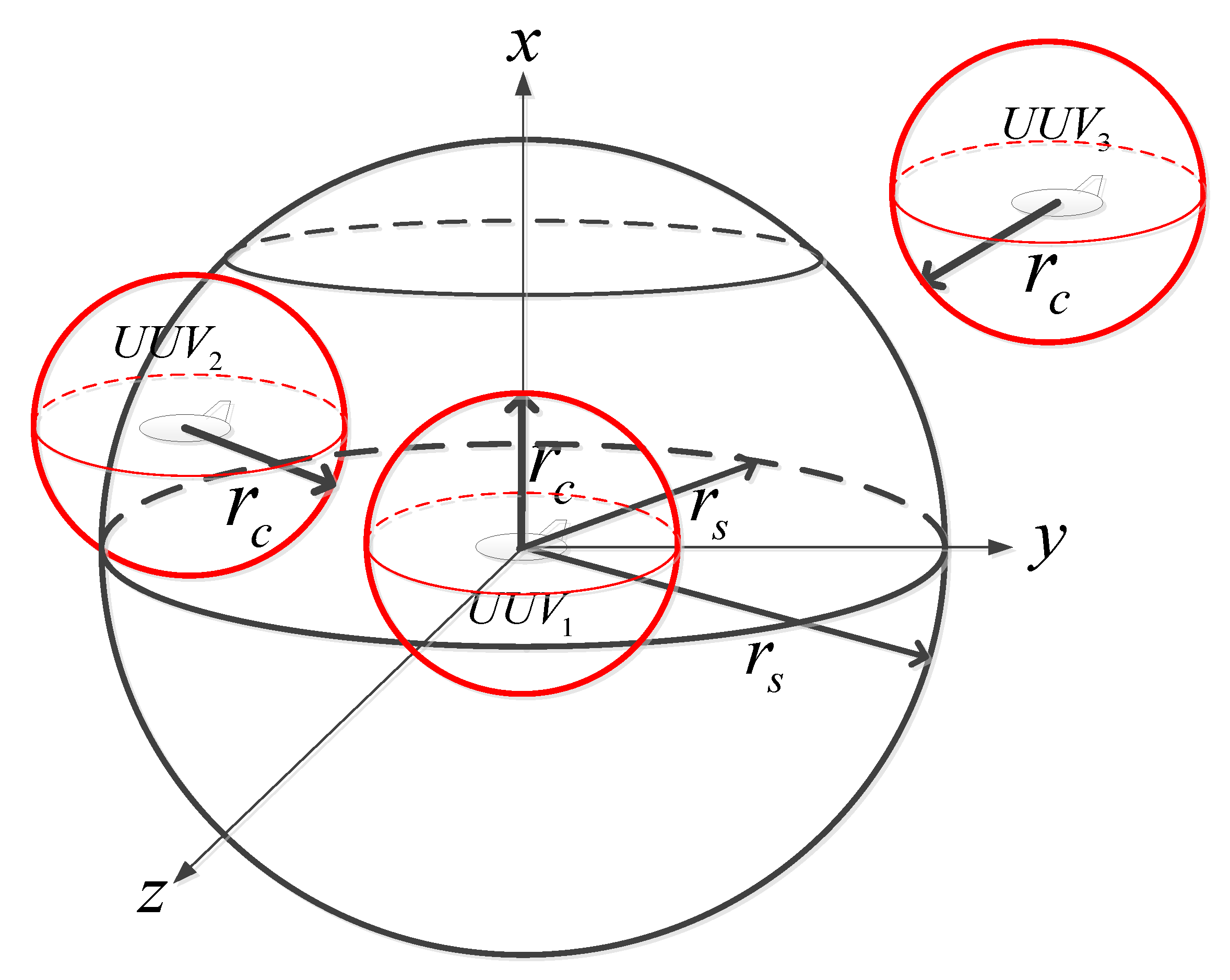
2.3. Artificial Potential Field and Virtual Repulsive

The APF method regards each UUV as a high-potential field. If any UUV is close to its neighbor, the repulsive force will repel the UUV away from the other UUV’s potential field. There are two advantages to collision avoidance by using the APF method. The first is that the individuals of multi-UUV systems can be separated from each other to avoid collisions. The second is that fewer parameters need to be debugged, and the controller design is much simpler than other collision avoidance methods. In practical engineering, the UUV is a rigid body with volume instead of a particle. Then, we assume that each UUV has the same structure and define the collision sphere and the collision avoidance sphere of a UUV, as shown in Figure 2. The collision avoidance sphere is defined by the black sphere with safe radius $r_s$. The collision sphere is shown by the red sphere with collision radius $r_c$. We define $\Vert d_{ij}\Vert =\sqrt{{\Vert x_i-x_j\Vert }^2+{\Vert y_i-y_j\Vert }^2+{\Vert z_i-z_j\Vert }^2}$ is the distance between ${\mathrm{U}\mathrm{U}\mathrm{V}}_i$ and ${\mathrm{U}\mathrm{U}\mathrm{V}}_j$. Shi [26] concludes that UUV $j$ is a collision avoidance neighbor $N_i^c$ of UUV $i$, while $\Vert d_{ij}\Vert \le r_s$. When $\Vert d_{ij}\Vert \le 2r_c$, collision occurs between ${\mathrm{U}\mathrm{U}\mathrm{V}}_i$ and ${\mathrm{U}\mathrm{U}\mathrm{V}}_j$.

To ensure that no collision occurs among the UUVs, an artificial potential function ${\delta }_{ij}(d)$ and an action function $\varsigma (d)$ are defined as:

$${\delta }_{ij}(d)={\displaystyle {\int }_{r_s}^d\varsigma (s)ds}$$

(7)

$$\varsigma (d)=\left\{\begin{array}{cc}-\frac{{\overline{\beta }}^c{}_i}{d^2}& d\in (2r_c,r_s)\\ 0& d\in [r_s,\propto )\end{array}\right\}$$

(8)

where ${\overline{\beta }}^c{}_i>0$ is a design parameter. When ${\overline{\beta }}^c{}_i$ is large enough and $d\to 2r_c$ or $d\to 0$, the potential function ${\delta }_{ij}(d)$ will tend to infinity. Thus, the repulsive force for collision avoidance is:

$${\tau }_i^{ca}={\beta }_{{}_i}^c{\displaystyle \sum _{j\in N_i^c}-{\nabla }_{p_i}}{\delta }_{ij}(d)=-{\beta }_{{}_i}^c{\displaystyle \sum _{j\in N_i^c}\varsigma (\Vert d_{ij}\Vert )}\frac{d_{ij}}{\Vert d_{ij}\Vert }$$

(9)

where $-{\nabla }_{p_i}$ denotes a negative gradient along $p_i$, and ${\beta }_{{}_i}^c$ is a positive gain parameter.

2.4. RBF Neural Network

The radial basis function neural network (RBFNN) is usually applied to approximate the unknown nonlinear functions because of its advantage of approximation property [14]. Then, the RBFNN is used to address the unknown disturbance in this article. The RBFNN $W^{*T}H(z)$ can approximate the continuous function of disturbance $W_i^{\omega }$ as:

$${\omega }_i=W_i{}^{*T}{H}_i(z_i)+{\phi }_i$$

(10)

where $\phi (z)\in {ℝ}^5$ is the estimation error, and $W^{*}=[W_1^{*},W_2^{*},\dots ,W_m^{*}]\in {ℝ}^{m\times 5}$ is the ideal constant weight. $H(z)$ represents the basis function vector described as:

$$H_k(z_i)=\exp \left[-\frac{{(z_i-{\ell }_k)}^T(z_i-{\ell }_k)}{{\kappa }_k^2}\right],k=1,2,\dots ,m$$

(11)

where ${\ell }_i$ is the center of the Gaussian kernel, and ${\kappa }_i$ denotes the width of the Gaussian kernel.

Define the error between the ideal weight and the estimated weight as:

$${\tilde{W}}_i={\widehat{W}}_i-W_i^{*}$$

(12)

where ${\widehat{W}}_i$ indicates the estimation of the ideal constant weight vector. Design the adaptive weight update law of the neural network as:

$${\dot{\widehat{W}}}_i=\frac{1}{c_i}[H_i(z_i){(e_{pi}+e_{vi})}^T-{\alpha }_i{\widehat{W}}_i]$$

(13)

where ${\alpha }_i$ is the designed positive parameter, and $c_i$ is a positive constants.

2.5. Control Objective

The goal of this paper is to design an adaptive controller for a multi-UUV system with collision avoidance. The control problems can be formally stated by the following objectives:

$$\begin{array}{l}\underset{t\to \infty }{\lim }\Vert p_i-p_l\Vert ={\epsilon }_i\\ \underset{t\to \infty }{\lim }\Vert v_i-v_l\Vert =0\\ \underset{t\to \infty }{\lim }\Vert d_{ij}^{}(t)\Vert \ge 2r_c\end{array}$$

(14)

where $d_{ij}(t)$ denotes the relative position variable between the UUV $i$ and its collision avoidance neighbor UUV $j$, and $\Vert ·\Vert$ is a Euclidean norm.

Assumption 1.

The disturbance is time-varying and bounded. Then, there exists a positive constant  ${\sigma }_{\omega }$, such that $\Vert \omega \Vert <{\sigma }_{\omega }$.

Assumption 2.

The velocity of UUVs and the virtual leader are not zero, e.g., $v_i\ne 0$ and $v_l\ne 0$. According to the characteristics of UUV, the velocity of UUVs is bounded, e.g., $\Vert v_i\Vert <{\sigma }_i^v$and $\Vert v_l\Vert <{\sigma }_l^v$, where ${\sigma }_i^v$and ${\sigma }_l^v$are positive constants.

Assumption 3.

At least one UUV can receive the information from the virtual leader, e.g., $\vartheta \ne 0$, where $\vartheta$is the communication matrix between the virtual leader and followers. The communication between the UUVs is connected, e.g., $A\ne 0$and $L\ne 0$.

Assumption 4.

The initial error in relative position and relative velocity of any two UUVs are bounded. e.g., $\Vert e_{pi}-e_{pj}\Vert <{\alpha }_p, \Vert e_{vi}-e_{vj}\Vert <{\alpha }_v$. ${\alpha }_p$and ${\alpha }_v$are positive finite values.

Lemma 1

[26]. $\vartheta =diag\{{\theta }_1,{\theta }_2,\dots ,{\theta }_n\}$ and ${\theta }_i\ge 0$. If the Laplacian matrix $L$ of the undirected graph is irreducible, then the eigenvalues of the matrix $L+\vartheta$ are positive definite, e.g., $\overline{L}=L+\vartheta >0$.

Lemma 2

[26]. $V(t)>0$ is a continuous function for any time, and the initial state of $V(0)$ is bounded. If the inequality $\dot{V}(t)>-\gamma V(t)+\Gamma$ holds with $\gamma >0, \Gamma >0$, then we have the following inequality:

$$V(t)\le V(0)e^{-\gamma t}+\frac{\Gamma }{\gamma }(1-e^{-\gamma t})$$

(15)

Lemma 3

[27]. $S(t)>0$ is a continuous function for any times, and the initial state of $S(0)$ is bounded. If the inequality holds $\dot{S}(t)>\lambda S(t)$ for $t>0, \lambda >0$, then we have the following inequality:

$$S(t)>e^{q(t-t_0)}S(t_0)$$

(16)

3. Main Results

3.1. Filtered High-Gain Observer Design

There are some conditions, such as guidance failure or the fault of facilities, where the states of the UUV cannot be obtained. To achieve the state estimation of the UUV formation, a filtered high-gain observer (FHGO) is designed for multi-UUV systems with measurement noise in the subsection. The main feature of the FHGO lies in its filtering capabilities, which allow obtaining relatively smooth estimates in the presence of noisy output measurements.

Let the UUV model be transformed into regular form:

$$\{\begin{array}{l}{\dot{p}}_i=v_i\hfill \\ {\dot{v}}_i={\tau }_i+{\omega }_i=f(p_i,v_i,{\tau }_i,{\omega }_i)\hfill \\ y_i=p_i+{\omega }_n\hfill \end{array}$$

(17)

The high-gain observer design will be performed according to the following assumption.

Assumption 5.

The states $p_i$and $v_i$are bounded. In addition, the noise${\omega }_n$is essentially a bounded function.

For comparison purposes, one recalls the equations of the standard high-gain observer (SHGO) proposed in [28]:

$$\{\begin{array}{l}{\dot{h}}_1=h_2+\frac{{\partial }_1}{\epsilon }(y-h_1)\hfill \\ {\dot{h}}_2=\widehat{f}(h_1,h_2,{\tau }_f)+\frac{{\partial }_2}{\epsilon }(y-h_1)\hfill \end{array}$$

(18)

where $h_1$ and $h_2$ denote the states of HGO, $\epsilon$ is a sufficiently small positive constant, ${\partial }_1$ and ${\partial }_2$ are chosen such that he roots of $s^2+{\partial }_{1}s+{\partial }_2$ have negative real parts, and $\widehat{f}(h_1,h_2,{\tau }_i)=f(h_1,h_2,{\tau }_i,0)$.

Inspired by Khalil [11], to improve the sensitivity properties of the observer with respect to measurement noise, an FHGO for UUV formation can be designed as follows

$$\{\begin{array}{l}{\dot{h}}_1=h_2+\frac{{\partial }_1}{\epsilon }(y_f-h_1)\hfill \\ {\dot{h}}_2=\widehat{f}(h_1,h_2,{\tau }_f)+\frac{{\partial }_2}{\epsilon }(y_f-h_1)\hfill \\ T_f\dot{z}=A_{f}z+B_{f}y\hfill \\ y_f=C_{f}z\hfill \end{array}$$

(19)

where $T_f$ is the time constant, and $A_f$, $B_f$ and $C_f$ are gain matrices such that $C_f{A}_f^{-1}{B}_f=-I$.

Theorem 1.

For the FHGO (21), there exists a positive constant $\beta$, arbitrarily small positive number $\overline{\mu }$and a finite time $T(\overline{\mu })$such that $\Vert \tilde{\eta }\Vert =\Vert \eta -h\Vert \le \overline{\mu }\beta$for $t\ge t_0+T(\overline{\mu })$, where $h={[h_1^{},h_2^{}]}^T$, $\eta ={[p,v]}^T$.

Proof of Theorem 1.

The following auxiliary variables are defined

$$\{\begin{array}{l}{T}_f{\dot{q}}_f=A_f{q}_f+B_f{\omega }_n\hfill \\ T_f{\dot{p}}_f=A_f{p}_f+B_{f}p\hfill \end{array}$$

(20)

Obviously, according to the above definition, $C_f{q}_f$ is the filtered signal of measurement noise ${\omega }_n$, which is denoted by ${\omega }_n{}_f$. Thus, we have $z_f=p_f+q_f$. Define the estimation errors $\tilde{p}=p-h_1$, $\tilde{v}=v-h_2$. Then, we have

$$\{\begin{array}{l}\dot{\tilde{p}}=\tilde{v}-\frac{{\alpha }_1}{∍}(C_f{z}_f-h_1)\hfill \\ \dot{\tilde{v}}=f(p,v,{\tau }_i,\omega )-\widehat{f}(h_1,h_2,{\tau }_f)-\frac{{\alpha }_2}{{∍}^2}(C_f{z}_f-h_1)\hfill \end{array}$$

(21)

According to the definition of $z_f$, we can obtain the detailed expansion of $C_f{z}_f-h_1$:

$$C_f{z}_f-h_1=C_f{\sigma }_1+C_f{q}_f+\tilde{p}$$

(22)

where ${\sigma }_1=p_f+A_f^{-1}{B}_{f}p$. Substitute the above Equation (24) into the error dynamics (23), we obtain:

$$\{\begin{array}{l}\dot{\tilde{p}}=\tilde{v}-\frac{{\partial }_1}{∍}(C_f{\sigma }_1+C_f{q}_f+\tilde{p})\hfill \\ \dot{\tilde{v}}=f(p,v,\tau ,\omega )-\widehat{f}(h_1,h_2,{\tau }_f)-\frac{{\partial }_2}{{∍}^2}(C_f{\sigma }_1+C_f{q}_f+\tilde{p})\hfill \end{array}$$

(23)

Now, consider the following change of coordinate

$$\{\begin{array}{l}{\varphi }_1=(\tilde{p}+C_f{\sigma }_1)/∍\hfill \\ {\varphi }_2=\tilde{v}+C_f{\sigma }_2\hfill \end{array}$$

(24)

where ${\sigma }_2={\dot{\sigma }}_1$. Taking derivative to the (24)

$$\{\begin{array}{l}∍{\dot{\varphi }}_1=(\dot{\tilde{p}}+C_f{\sigma }_2)={\varphi }_2-{\partial }_1{\varphi }_1-{\partial }_1{w}_n/∍\hfill \\ ∍{\dot{\varphi }}_2=∍\dot{\tilde{v}}+∍C_f{\dot{\sigma }}_2=-{\partial }_2{\varphi }_1-{\partial }_2{w}_n/∍+∍(C_f{p}_f{}^{(2)}-\widehat{f}(h_1,h_2,{\tau }_f))\hfill \end{array}$$

(25)

Then, it can be written in the compact form as:

$$∍\dot{\varphi }=A_f\varphi +B_f(p_f{}^{(2)},\widehat{f}(h_1,h_2,{\tau }_f),w_n)$$

(26)

where $\varphi ={[{\varphi }_1,{\varphi }_2]}^T$, $A_f=\left[\begin{array}{cc}-{\partial }_1{I}_3& I_3\\ -{\partial }_2{I}_3& 0_3\end{array}\right]$, $B_f(p_f{}^{(2)},\widehat{f}(h_1,h_2,{\tau }_f),w_n)=\left[\begin{array}{c}-{\partial }_1{w}_n/∍\\ -{\partial }_2{w}_n/∍+∍(C_f{p}_f{}^{(2)}-\widehat{f}(h_1,h_2,{\tau }_f))\end{array}\right]$.

Consider the Lyapunov function $V$ as

$$V_O={\varphi }^T{P}_f\varphi$$

(27)

where $A_f{}^T{P}_f+P_f{A}_f=-I$. Taking the derivative of the Lyapunov function and inserting (26) leads to:

$$\begin{array}{c}∍{\dot{V}}_O={\varphi }^T(P_f{A}_f+A_f^T{P}_f)\varphi +2{\varphi }^T{P}_f{B}_f(p_f{}^{(2)},\widehat{f}(h_1,h_2,{\tau }_f),w_n)\hfill \\ \le -{\varphi }^T\varphi +2\Vert \varphi \Vert \Vert P_f\Vert (\left[\begin{array}{c}{0}_{3,1}\\ ∍\Vert C_f{p}_f{}^{(2)}-\widehat{f}(h_1,h_2,{\tau }_f)\Vert \end{array}\right]+\left[\begin{array}{c}\Vert {\partial }_1{w}_n/∍\Vert \\ \Vert {\partial }_2{w}_n/∍\Vert \end{array}\right])\hfill \end{array}$$

(28)

By the definition of $p_f$ in (20), we have

$$T_f{\dot{p}}_f{}^{(2)}=A_f{p}_f{}^{(2)}+B_{f}f(p,v,\tau ,\omega )$$

(29)

Then, by the negative definiteness of $A_f$ and Assumption 1, it can be shown that $p_f{}^{(2)}$ is ultimately bounded by $O(T_f)$. Furthermore, we can deduce that $\Vert C_f{P}_f{}^{(2)}-\widehat{f}(h_1,h_2,{\tau }_f)\Vert$ is bounded by some constant ${\overline{b}}_n$, and

$$∍{\dot{V}}_O\le -{\varphi }^T\varphi +c_{{}_1}^f∍{\overline{b}}_n\Vert \varphi \Vert +c_{{}_2}^f{\overline{w}}_f{∍}^{-1}\Vert \varphi \Vert$$

(30)

where $c_{{}_1}^f=2\Vert P_f\Vert$, $c_{{}_2}^f=2\Vert P_f\Vert {\partial }_3$, ${\partial }_3=\max \{2{\partial }_1,2{\partial }_2\}$.

Using the fact that ${\lambda }_{min}(P_f){\varphi }^T\varphi \le V\le {\lambda }_{max}(P_f){\varphi }^T\varphi$ and ${\dot{V}}_O=2\sqrt{V_O}d\sqrt{V_O}/dt$, after some expansions and simplifications, we arrive at

$$2∍\sqrt{V_O}d\sqrt{V_O}/dt\le -l_0{V}_O+l_1∍{\overline{b}}_n\sqrt{V_O}+l_2{∍}^{-1}{\overline{w}}_n\sqrt{V_O}$$

(31)

where $l_0={\lambda }_{max}{(P_f)}^{-1}$, $l_1=c_{{}_1}^f{\lambda }_{min}{(P_f)}^{-1/2}$, $l_2=c_{{}_2}^f{\lambda }_{min}{(P_f)}^{-1/2}$. After computations, we obtain

$$\frac{d\sqrt{V_O}}{dt}\le -\frac{l_0}{2∍}\sqrt{V}+\frac{l_1}{2}{\overline{b}}_n+\frac{l_2}{2{∍}^2}{\overline{w}}_n$$

(32)

It can be verified that

$$\sqrt{V_O}\le \frac{l_1∍{\overline{b}}_n}{l_0}+\frac{l_2{\overline{w}}_n}{ϵl_0}+e^{-l_{0}t/2∍}\sqrt{V_O(0)}$$

(33)

In the light of $V_O={\varphi }^{T}P\varphi$, some positive constants $r_1$, $r_2$, $r_3$ must exist such that:

$$\Vert \varphi \Vert \le r_1∍{\overline{b}}_n+r_2{∍}^{-1}{\overline{w}}_n+e^{-l_{0}t/2∍}{r}_3\Vert \varphi (0)\Vert$$

(34)

Recall that

$$\{\begin{array}{l}\tilde{p}=∍{\varphi }_1-C_f{\sigma }_1\hfill \\ \tilde{v}={\varphi }_2-C_f{\sigma }_2\hfill \end{array}$$

(35)

Obviously, if ${\sigma }_1$ and ${\sigma }_2$ are bounded, then the uniform ultimate boundedness of tracking error can be obtained. The derivative of ${\sigma }_1$ and ${\sigma }_2$ can be derived as

$$\{\begin{array}{l}{T}_f{\dot{\sigma }}_1=A_f{\sigma }_1+T{A}_f^{-1}{B}_{f}v\hfill \\ T_f{\dot{\sigma }}_2=A_f{\sigma }_2+T{A}_f^{-1}{B}_{f}f\hfill \end{array}$$

(36)

Then, by Assumption 1, it can be shown that ${\sigma }_1$ and ${\sigma }_2$ are ultimately bounded by $O(T_f)$. After some computations, we obtain

$$\{\begin{array}{ll}\Vert \tilde{p}\Vert \le \hfill & r_1{∍}^2{\overline{b}}_n+r_2{\overline{w}}_n+(1+r_3{e}^{-l_{0}t/2∍})r_{4}O(T_f)\hfill \\ \hfill & +e^{-l_{0}t/2∍}{r}_3\Vert \tilde{\eta }(0)\Vert \hfill \\ \Vert \tilde{v}\Vert \le \hfill & r_1∍{\overline{b}}_n+r_2{∍}^{-1}{\overline{w}}_n+(1+r_3{∍}^{-1}{e}^{-l_{0}t/2∍})r_4\hfill \\ \hfill & O(T_f)+e^{-l_{0}t/2∍}{r}_3{∍}^{-1}\Vert \tilde{\eta }(0)\Vert \hfill \end{array}$$

(37)

where $r_4=\Vert C_f\Vert$. Then, by choosing a constant $\beta =\max \left\{2{\beta }_1,2{\beta }_2\right\}$ and $\overline{\mu }=\max \{∍,O(T_f)\}$, where ${\beta }_1=\max \{r_1{\overline{b}}_n,r_2,2r_4\}$, ${\beta }_2=\max \{r_1{\overline{b}}_n,r_2,2r_4\}$, time $T(\overline{\mu })$ must exists such that $\Vert \tilde{\eta }\Vert \le \overline{\mu }\beta$ for $t\ge t_0+T(\overline{\mu })$. This completes the proof. □

Remark 1.

It should be noted that when the measurement noise bound ${\overline{\omega }}_n$is small enough,$\overline{\mu }$can always be arbitrarily small by selecting the appropriate time constant$T_f$and observer parameter$∍$. Therefore, the estimation errors of the observer are guaranteed to be bounded. Moreover, according to Theorem 1, the accurate estimations of the position vector p and velocity vector v of the ship can be obtained through the appropriate coordinate transformation of the state of the FHGO:

$$\hslash :=\gamma h\to {[\eta ,\nu ]}^T$$

(38)

where$\gamma =diag(I_3,I_3)$. The FHGO designed in this subsection will be used to accurately estimate the states of multi-UUV systems in the following sections.

Define error of the whole system with state observer as:

$$\begin{array}{cc}{\widehat{e}}_{pi}& ={\displaystyle \sum _{j\in N_i^c}{a}_{ij}((h_{1i}-h_{1j})-({\epsilon }_i-{\epsilon }_j))}+{\theta }_i(h_{1i}-p_l-{\epsilon }_i)\hfill \\ & =e_{pi}-({\displaystyle \sum _{j\in N_i^c}{a}_{ij}({\tilde{p}}_i-{\tilde{p}}_j)}+{\theta }_i{\tilde{p}}_i)\hfill \\ {\widehat{e}}_{vi}& ={\displaystyle \sum _{j\in N_i^c}{a}_{ij}(v_i-v_j)}+{\theta }_i(v_i-v_l)\hfill \\ & =e_{vi}-({\displaystyle \sum _{j\in N_i^c}{a}_{ij}({\tilde{v}}_i-{\tilde{v}}_j)}+{\theta }_i{\tilde{v}}_i)\hfill \end{array}$$

(39)

3.2. Adaptive Neural Network Formation Control with Collision Avoidance under Unknown Disturbances

The formation control law of the multi-UUVs is defined as:

$${\tau }_i^f=-{\widehat{W}}_i^T{H}_i(z_i)-k_i({\widehat{e}}_{vi}+{\widehat{e}}_{pi})$$

(40)

Combining (9) with (40), we can obtain the formation controller based on a high-gain observer with collision avoidance under unknown disturbances is designed as

$${\tau }_i={\tau }_i^f+{\tau }_i^{ca}$$

(41)

Proof of the Stability of the System.

Define the Lyapunov function as follows:

$$V_C=\frac{1}{2}{\overline{Z}}^T(Q\otimes I_5)\overline{Z}+\frac{1}{2}{\displaystyle \sum _{i=1}^n{c}_i{\tilde{W}}_i^T{\tilde{W}}_i}$$

(42)

where $\otimes$ represents the Kronecker product. Define the derivatives of the error variable as follows:

$$\dot{\overline{Z}}=-[U\otimes I_5]\overline{Z}+[\begin{array}{c}{O}_{5n}\\ T_i^{\tau }\end{array}]+[\begin{array}{c}{O}_{5n}\\ W_i^{\omega }\end{array}]-[\begin{array}{c}{O}_{5n}\\ G_l^g\end{array}]$$

(43)

where $U=\left[\begin{array}{cc}{O}_n& -I_n\\ O_n& O_n\end{array}\right]$, $T_i^{\tau }={[{\tau }_1^T,\dots ,{\tau }_n^T]}^T$, $W_i^{\omega }={[{\omega }_1^T,\dots ,{\omega }_n^T]}^T$, $G_l^g={[g_l^T,\dots ,g_l^T]}^T$. Taking the time derivative of the Lyapunov function, we obtain

$$\begin{array}{cc}{\dot{V}}_C& ={\overline{Z}}^T(Q\otimes I_5)\dot{\overline{Z}}+{\displaystyle \sum _{i=1}^n{c}_i{\tilde{W}}_i^T{\dot{\widehat{W}}}_i}\hfill \\ & =-\frac{1}{2}{\overline{Z}}^T((U^{T}Q+QU)\otimes I_5)\overline{Z}+{\overline{Z}}^T(Q\otimes I_5)([\begin{array}{c}{O}_{5n}\\ T_i^{\tau }\end{array}]+[\begin{array}{c}{O}_{5n}\\ W_i^{\omega }\end{array}]-[\begin{array}{c}{O}_{5n}\\ G_l^g\end{array}])+{\displaystyle \sum _{i=1}^n{c}_i{\tilde{W}}_i^T{\dot{\widehat{W}}}_i}\hfill \end{array}$$

(44)

where $Q=\left[\begin{array}{cc}2\overline{L}& \overline{L}\\ \overline{L}& \overline{L}\end{array}\right]$. Substituting (9), (13) and (40) becomes

$$\begin{array}{cc}{\dot{V}}_C& =-{\overline{Z}}^T(\left[\begin{array}{cc}{O}_n& -\overline{L}\\ -\overline{L}& -\overline{L}\end{array}\right]\otimes I_5)\overline{Z}+{\displaystyle \sum _{i=1}^n{\tilde{W}}_i^T(H_i(z_i){({\widehat{e}}_{pi}+{\widehat{e}}_{vi})}^T-{\alpha }_i{\widehat{W}}_i)}-{\displaystyle \sum _{i=1}^n{(e_{pi}+e_{vi})}^T{g}_l(t)}\hfill \\ & +{\displaystyle \sum _{i=1}^n{(e_{pi}+e_{vi})}^T{\omega }_i+}{\displaystyle \sum _{i=1}^n{(e_{pi}+e_{vi})}^T(}-{\widehat{W}}_i^T{H}_i(z_i)-k_i({\widehat{e}}_{vi}+{\widehat{e}}_{pi})-{\beta }_{{}_i}^c{\displaystyle \sum _{j\in N_i^c}\varsigma (\Vert d_{ij}\Vert )}\frac{d_{ij}}{\Vert d_{ij}\Vert })\hfill \\ & =-{\overline{Z}}^T(\left[\begin{array}{cc}{O}_n& -\overline{L}\\ -\overline{L}& -\overline{L}\end{array}\right]\otimes I_5)\overline{Z}+{\displaystyle \sum _{i=1}^n{\tilde{W}}_i^T(H_i(z_i){({\widehat{e}}_{pi}+{\widehat{e}}_{vi})}^T-{\alpha }_i{\widehat{W}}_i)}-{\displaystyle \sum _{i=1}^n{(e_{pi}+e_{vi})}^T{g}_l(t)}\hfill \\ & +{\displaystyle \sum _{i=1}^n{(e_{pi}+e_{vi})}^T(W_i{}^{*T}{H}_i(z_i)+{\phi }_i)+}{\displaystyle \sum _{i=1}^n{(e_{pi}+e_{vi})}^T(}-{\widehat{W}}_i^T{H}_i(z_i)-k_i({\widehat{e}}_{vi}+{\widehat{e}}_{pi}))\hfill \\ & -{\displaystyle \sum _{i=1}^n{(e_{pi}+e_{vi})}^T(}{\beta }_{{}_i}^c{\displaystyle \sum _{j\in N_i^c}-{\nabla }_{p_i}}{\delta }_{ij}(d))\hfill \end{array}$$

(45)

For an undirected graph, the repulsive forces between UUVs are equal and opposite in direction [29]. Therefore, ${\beta }_{{}_i}^c{\displaystyle \sum _{i=1}^n{(e_{pi}+e_{vi})}^T}{\displaystyle \sum _{j\in N_i^c}-{\nabla }_{p_i}}{\delta }_{ij}(d)=0$. Then, substituting (38), we obtain

$$\begin{array}{cc}{\dot{V}}_C& =-{\overline{Z}}^T(\left[\begin{array}{cc}{O}_n& -\overline{L}\\ -\overline{L}& -\overline{L}\end{array}\right]\otimes I_n)\overline{Z}+{\displaystyle \sum _{i=1}^n{(e_{pi}+e_{vi})}^T({\widehat{W}}_i^T{H}_i(z_i)-{\tilde{W}}_i^T{H}_i(z_i)+{\phi }_i)}\hfill \\ & +{\displaystyle \sum _{i=1}^n{\tilde{W}}_i^T(H_i(z_i){(e_{pi}+e_{vi})}^T-{\alpha }_i{\widehat{W}}_i)}+{\displaystyle \sum _{i=1}^n{(e_{pi}+e_{vi})}^T(}-{\widehat{W}}_i^T{H}_i(z_i)-k_i(e_{vi}+e_{pi}))\hfill \\ & +{\displaystyle \sum _{i=1}^n{\tilde{W}}_i^T(-{\displaystyle \sum _{j\in N_i^c}{a}_{ij}({\tilde{p}}_i-{\tilde{p}}_j)}+{\theta }_i{\tilde{p}}_i)-({\displaystyle \sum _{j\in N_i^c}{a}_{ij}({\tilde{v}}_i-{\tilde{v}}_j)}+{\theta }_i{\tilde{v}}_i)))}-{\displaystyle \sum _{i=1}^n{(e_{pi}+e_{vi})}^T{g}_l(t)}\hfill \\ & +{\displaystyle \sum _{i=1}^n{(e_{pi}+e_{vi})}^T(-}({\displaystyle \sum _{j\in N_i^c}{a}_{ij}({\tilde{v}}_i-{\tilde{v}}_j)}+{\theta }_i{\tilde{v}}_i)-({\displaystyle \sum _{j\in N_i^c}{a}_{ij}({\tilde{p}}_i-{\tilde{p}}_j)}+{\theta }_i{\tilde{p}}_i))\hfill \\ & =-{\overline{Z}}^T(\left[\begin{array}{cc}{O}_n& -\overline{L}\\ -\overline{L}& -\overline{L}\end{array}\right]\otimes I_n)\overline{Z}-{\displaystyle \sum _{i=1}^n{(e_{pi}+e_{vi})}^T{g}_l(t)}-{\displaystyle \sum _{i=1}^n{k}_i{\Vert e_{pi}+e_{vi}\Vert }^2}\hfill \\ & +{\displaystyle \sum _{i=1}^n{\tilde{W}}_i^T(-{\displaystyle \sum _{j\in N_i^c}{a}_{ij}({\tilde{p}}_i-{\tilde{p}}_j)}-{\displaystyle \sum _{j\in N_i^c}{a}_{ij}({\tilde{v}}_i-{\tilde{v}}_j)}-{\theta }_i({\tilde{p}}_i+{\tilde{v}}_i))}-{\displaystyle \sum _{i=1}^n{\alpha }_i{\tilde{W}}_i^T{\widehat{W}}_i}\hfill \\ & +{\displaystyle \sum _{i=1}^n{(e_{pi}+e_{vi})}^T(}-{\displaystyle \sum _{j\in N_i^c}{a}_{ij}({\tilde{p}}_i-{\tilde{p}}_j)}-{\displaystyle \sum _{j\in N_i^c}{a}_{ij}({\tilde{v}}_i-{\tilde{v}}_j)}-{\theta }_i({\tilde{p}}_i+{\tilde{v}}_i))+{\displaystyle \sum _{i=1}^n{(e_{pi}+e_{vi})}^T{\phi }_i}\hfill \end{array}$$

(46)

Based on the Young’s inequality

$$\begin{array}{cc}\hfill -{\displaystyle \sum _{i=1}^n{\alpha }_i{\tilde{W}}_i^T{\widehat{W}}_i}\le & -\frac{1}{2}{\alpha }_i{\tilde{W}}^2+-\frac{1}{2}{\alpha }_i{W}^{*2}\hfill \\ \hfill -{\displaystyle \sum _{i=1}^n{(e_{pi}+e_{vi})}^T{g}_l(t)}\le & \frac{1}{2}{♭}_{i,8}^{}{\Vert e_{pi}+e_{vi}\Vert }^2+\frac{{ð}^2}{2{♭}_{i,8}^{}}\hfill \\ \hfill -{\displaystyle \sum _{i=1}^n{(e_{pi}+e_{vi})}^T{\displaystyle \sum _{j\in N_i^c}{a}_{ij}({\tilde{v}}_i-{\tilde{v}}_j)}}\le & \frac{1}{2}({♭}_{i,1}^{}{\Vert e_{pi}+e_{vi}\Vert }^2+\frac{1}{{♭}_{i,1}^{}}{({\tilde{v}}_i-{\tilde{v}}_j)}^T{A}^{-1}A({\tilde{v}}_i-{\tilde{v}}_j))\hfill \\ \hfill -{\displaystyle \sum _{i=1}^n{(e_{pi}+e_{vi})}^T{\displaystyle \sum _{j\in N_i^c}{a}_{ij}({\tilde{p}}_i-{\tilde{p}}_j)}}\le & \frac{1}{2}({♭}_{i,2}^{}{\Vert e_{pi}+e_{vi}\Vert }^2+\frac{1}{{♭}_{i,2}^{}}{({\tilde{p}}_i-{\tilde{p}}_j)}^T{A}^{-1}A({\tilde{p}}_i-{\tilde{p}}_j))\hfill \\ \hfill -{\displaystyle \sum _{i=1}^n{(e_{pi}+e_{vi})}^T{\displaystyle \sum _{j\in N_i^c}{\theta }_i({\tilde{p}}_i+{\tilde{v}}_i)}}\le & \frac{1}{2}({♭}_{i,4}^{}{\Vert e_{pi}+e_{vi}\Vert }^2+\frac{1}{{♭}_{i,4}^{}}{({\tilde{p}}_i+{\tilde{v}}_i)}^T{\vartheta }^{-1}\vartheta ({\tilde{p}}_i+{\tilde{v}}_i))\hfill \\ \hfill -{\displaystyle \sum _{i=1}^n{(e_{pi}+e_{vi})}^T{\displaystyle \sum _{j\in N_i^c}{\phi }_i}}\le & \frac{1}{2}({♭}_{i,7}^{}{\Vert e_{pi}+e_{vi}\Vert }^2+\frac{1}{{♭}_{i,7}^{}}{\phi }_i{}^T{\phi }_i)\hfill \end{array}$$

(47)

$$\begin{array}{cc}\hfill -{\displaystyle \sum _{i=1}^n{\tilde{W}}_i^T{\displaystyle \sum _{j\in N_i^c}{a}_{ij}({\tilde{v}}_i-{\tilde{v}}_j)}}\le & \frac{1}{2}({♭}_{i,4}^{}{\tilde{W}}_i^T{\tilde{W}}_i^{}+\frac{1}{{♭}_{i,4}^{}}{({\tilde{v}}_i-{\tilde{v}}_j)}^T{A}^{-1}A({\tilde{v}}_i-{\tilde{v}}_j))\hfill \\ \hfill -{\displaystyle \sum _{i=1}^n{\tilde{W}}_i^T{\displaystyle \sum _{j\in N_i^c}{a}_{ij}({\tilde{p}}_i-{\tilde{p}}_j)}}\le & \frac{1}{2}({♭}_{i,5}^{}{\tilde{W}}_i^T{\tilde{W}}_i^{}+\frac{1}{{♭}_{i,5}^{}}{({\tilde{p}}_i-{\tilde{p}}_j)}^T{A}^{-1}A({\tilde{p}}_i-{\tilde{p}}_j))\hfill \\ \hfill -{\displaystyle \sum _{i=1}^n{\tilde{W}}_i^T{\displaystyle \sum _{j\in N_i^c}{\theta }_i({\tilde{p}}_i+{\tilde{v}}_i)}}\le & \frac{1}{2}({♭}_{i,6}^{}{\tilde{W}}_i^T{\tilde{W}}_i^{}+\frac{1}{{♭}_{i,6}^{}}{({\tilde{p}}_i+{\tilde{v}}_i)}^T{\vartheta }^{-1}\vartheta ({\tilde{p}}_i+{\tilde{v}}_i))\hfill \end{array}$$

(48)

where ${♭}_{i,j}$ is a positive constant, and $j=1,2,\dots ,7$. Then, we can obtain

$$\begin{array}{cc}{\dot{V}}_C& \le -{\overline{Z}}^T(\left[\begin{array}{cc}{O}_n& -\overline{L}\\ -\overline{L}& -\overline{L}\end{array}\right]\otimes I_n)\overline{Z}+\frac{1}{2}({♭}_{i,1}{\Vert e_{pi}+e_{vi}\Vert }^2+\frac{1}{{♭}_{i,1}}{({\tilde{v}}_i-{\tilde{v}}_j)}^T{A}^{-1}A({\tilde{v}}_i-{\tilde{v}}_j))\hfill \\ & +\frac{1}{2}({♭}_{i,2}{\Vert e_{pi}+e_{vi}\Vert }^2+\frac{1}{{♭}_{i,2}}{({\tilde{p}}_i-{\tilde{p}}_j)}^T{A}^{-1}A({\tilde{p}}_i-{\tilde{p}}_j))-{\displaystyle \sum _{i=1}^n{k}_i{\Vert e_{pi}+e_{vi}\Vert }^2}\hfill \\ & +\frac{1}{2}({♭}_{i,3}{\Vert e_{pi}+e_{vi}\Vert }^2+\frac{1}{{♭}_{i,3}}{({\tilde{p}}_i+{\tilde{v}}_i)}^T{\vartheta }^{-1}\vartheta ({\tilde{p}}_i+{\tilde{v}}_i))+\frac{{♭}_{i,8}}{2}{\Vert e_{pi}+e_{vi}\Vert }^2+{\displaystyle \sum _{i=1}^n\frac{{ð}^2}{2{♭}_{i,8}}}\hfill \\ & +\frac{1}{2}({♭}_{i,4}{\tilde{W}}_i^T{\tilde{W}}_i^{}+\frac{1}{{♭}_{i,4}}{({\tilde{v}}_i-{\tilde{v}}_j)}^T{A}^{-1}A({\tilde{v}}_i-{\tilde{v}}_j))-\frac{1}{2}({♭}_{i,7}{\Vert e_{pi}+e_{vi}\Vert }^2+\frac{1}{{♭}_{i,7}}{\phi }_i{}^T{\phi }_i)\hfill \\ & +\frac{1}{2}({♭}_{i,5}^{}{\tilde{W}}_i^T{\tilde{W}}_i^{}+\frac{1}{{♭}_{i,5}^{}}{({\tilde{p}}_i-{\tilde{p}}_j)}^T{A}^{-1}A({\tilde{p}}_i-{\tilde{p}}_j))-\frac{1}{2}{\alpha }_i{\tilde{W}}^2+\frac{1}{2}{\alpha }_i{W}^{*2}\hfill \\ & +\frac{1}{2}({♭}_{i,6}^{}{\tilde{W}}_i^T{\tilde{W}}_i^{}+\frac{1}{{♭}_{i,6}^{}}{({\tilde{p}}_i+{\tilde{v}}_i)}^T{\vartheta }^{-1}\vartheta ({\tilde{p}}_i+{\tilde{v}}_i))\hfill \\ & =-{\overline{Z}}^T(\left[\begin{array}{cc}{O}_n& -\overline{L}\\ -\overline{L}& -\overline{L}\end{array}\right]\otimes I_n)\overline{Z}-{\displaystyle \sum _{i=1}^n(k_i-\frac{{♭}_{i,1}^{}+{♭}_{i,2}^{}+{♭}_{i,3}^{}-{♭}_{i,7}^{}+{♭}_{i,8}^{}}{2}){\Vert e_{pi}+e_{vi}\Vert }^2}\hfill \\ & -\frac{1}{2}{\displaystyle \sum _{i=1}^n({\alpha }_i-{♭}_{i,4}^{}-{♭}_{i,5}^{}-{♭}_{i,6}^{}){\tilde{W}}^2}+\frac{1}{2}{\displaystyle \sum _{i=1}^n{\alpha }_i{W}^{*2}}+{\displaystyle \sum _{i=1}^n\frac{{ð}^2}{2{♭}_{i,8}^{}}}+\frac{1}{2}(\frac{1}{{♭}_{i,1}^{}}+\frac{1}{{♭}_{i,4}^{}}){\Vert {\tilde{v}}_i-{\tilde{v}}_j\Vert }^2\hfill \\ & +\frac{1}{2}(\frac{1}{{♭}_{i,2}^{}}+\frac{1}{{♭}_{i,5}^{}}){\Vert {\tilde{p}}_i-{\tilde{p}}_j\Vert }^2+\frac{1}{2}(\frac{1}{{♭}_{i,3}^{}}+\frac{1}{{♭}_{i,6}^{}}){\Vert {\tilde{p}}_i+{\tilde{v}}_i\Vert }^2-\frac{1}{2{♭}_{i,7}^{}}{\Vert {\phi }_i\Vert }^2\hfill \end{array}$$

(49)

Choose ${\rho }_{{}_{i,1}}^{}\le k_i-\frac{{♭}_{i,1}^{}+{♭}_{i,2}^{}+{♭}_{i,3}^{}-{♭}_{i,7}^{}+{♭}_{i,8}^{}}{2}>0$ and ${\rho }_{{}_{i,2}}^{}\le {\alpha }_i-{♭}_{i,4}^{}-{♭}_{i,5}^{}-{♭}_{i,6}^{}>0$. ${\phi }_i$, ${\tilde{v}}_i$, ${\tilde{p}}_i$ are the error terms that are bounded. $\frac{{ð}^2}{2{♭}_{i,8}^{}}$ and ${\alpha }_i{W}^{*2}$ are constants. Thus, let $\begin{array}{cc}\Gamma & =\frac{1}{2}[(\frac{1}{{♭}_{i,1}^{}}+\frac{1}{{♭}_{i,4}^{}}){\Vert {\tilde{v}}_i-{\tilde{v}}_j\Vert }^2+(\frac{1}{{♭}_{i,2}^{}}+\frac{1}{{♭}_{i,5}^{}}){\Vert {\tilde{p}}_i-{\tilde{p}}_j\Vert }^2+(\frac{1}{{♭}_{i,3}^{}}+\frac{1}{{♭}_{i,6}^{}}){\Vert {\tilde{p}}_i+{\tilde{v}}_i\Vert }^2+\frac{1}{{♭}_{i,7}^{}}{\Vert {\phi }_i\Vert }^2]\hfill \\ & +\frac{1}{2}{\displaystyle \sum _{i=1}^n{\alpha }_i{W}^{*2}}+{\displaystyle \sum _{i=1}^n\frac{{ð}^2}{2{♭}_{i,8}^{}}}\hfill \end{array}$.

Then, (47) can be written as:

$$\begin{array}{cc}{\dot{V}}_C& \le -{\overline{Z}}^T(\left[\begin{array}{cc}{O}_n& -\overline{L}\\ -\overline{L}& -\overline{L}\end{array}\right]\otimes I_n)\overline{Z}-{\displaystyle \sum _{i=1}^n{\rho }_{{}_{i,1}}^{}{\Vert e_{pi}+e_{vi}\Vert }^2}-\frac{1}{2}{\displaystyle \sum _{i=1}^n{\rho }_{{}_{i,2}}^{}{\tilde{W}}^2}+\Gamma \hfill \\ & =-{\overline{Z}}^T(({\rho }_{{}_{i,1}}^{}\left[\begin{array}{cc}{\overline{L}}^2& {\overline{L}}^2\\ {\overline{L}}^2& {\overline{L}}^2\end{array}\right]+\left[\begin{array}{cc}{O}_n& -\overline{L}\\ -\overline{L}& -\overline{L}\end{array}\right])\otimes I_n)\overline{Z}-\frac{1}{2}{\displaystyle \sum _{i=1}^n{\rho }_{{}_{i,2}}^{}{\tilde{W}}^2}+\Gamma \hfill \\ & ={\overline{Z}}^T(\left[\begin{array}{cc}{\rho }_{{}_{i,1}}^{}{\overline{L}}^2& {\rho }_{{}_{i,1}}^{}{\overline{L}}^2-\overline{L}\\ {\rho }_{{}_{i,1}}^{}{\overline{L}}^2-\overline{L}& {\rho }_{{}_{i,1}}^{}\overline{L}-{\overline{L}}^2\end{array}\right])\otimes I_n)\overline{Z}-\frac{1}{2}{\displaystyle \sum _{i=1}^n{\rho }_{{}_{i,2}}^{}{\tilde{W}}^2}+\Gamma \hfill \end{array}$$

(50)

According to [24], ${\rho }_{{}_{i,1}}^{}{\overline{L}}^2-({\rho }_{{}_{i,1}}^{}{\overline{L}}^2-\overline{L})={\overline{L}}^2>0,{\rho }_{{}_{i,1}}^{}{\overline{L}}^2-\overline{L}>0$, so the matrix $\left[\begin{array}{cc}{\rho }_{{}_{i,1}}^{}{\overline{L}}^2& {\rho }_{{}_{i,1}}^{}{\overline{L}}^2-\overline{L}\\ {\rho }_{{}_{i,1}}^{}{\overline{L}}^2-\overline{L}& {\rho }_{{}_{i,1}}^{}\overline{L}-{\overline{L}}^2\end{array}\right]>0$ such that

$$\begin{array}{cc}{\dot{V}}_C& \le -{\overline{Z}}^T(({\rho }_{{}_{i,1}}^{}\left[\begin{array}{cc}{\overline{L}}^2& {\overline{L}}^2\\ {\overline{L}}^2& {\overline{L}}^2\end{array}\right]+\left[\begin{array}{cc}{O}_n& -\overline{L}\\ -\overline{L}& -\overline{L}\end{array}\right])\otimes I_n)\overline{Z}-\frac{1}{2}{\displaystyle \sum _{i=1}^n{\rho }_{{}_{i,2}}^{}{\tilde{W}}^2}+\Gamma \hfill \\ & =-{\overline{Z}}^T(({\rho }_{{}_{i,1}}^{}\pounds +\Theta )\otimes I_n)\overline{Z}-\frac{1}{2}{\displaystyle \sum _{i=1}^n{\rho }_{{}_{i,2}}^{}{\tilde{W}}^2}+\Gamma \hfill \end{array}$$

(51)

By choosing ${\rho }_{{}_{i,1}}^{}>{\lambda }_{\min }^{\pounds }({\lambda }_{\min }^{\Theta }+\frac{\gamma }{2}{\lambda }_{\max }^Q)$, ${\lambda }_{\min }^{\pounds }$ and ${\lambda }_{\min }^{\Theta }$ are the smallest eigenvalue of the matrix $\pounds$ and $\Theta$, respectively, and ${\lambda }_{\max }^Q$ denotes the largest eigenvalue of the matrix $Q$. $\gamma =\min \{{\alpha }_1{c}_1,\dots ,{\alpha }_n{c}_n\}$.

Then, we can obtain

$$\begin{array}{cc}{\dot{V}}_C& \le -\frac{\gamma }{2}{\overline{Z}}^T(Q\otimes I_n)\overline{Z}-\frac{\gamma }{2}{\displaystyle \sum _{i=1}^n{\tilde{W}}^2}+\Gamma \hfill \\ & =-\gamma V_C+\Gamma \hfill \end{array}$$

(52)

According to Lemma 2, the inequality can be obtained as

$$V_C(t)\le V_C(0)e^{-\gamma t}+\frac{\Gamma }{\gamma }(1-e^{-\gamma t})$$

(53)

Then, the adaptive UUV formation system with disturbance achieves performance. □

Proof of Collision Avoidance.

Define an energy function:

$$S(t)=\frac{1}{2}{d}_{ij}^T(t)d_{ij}(t)+\frac{1}{2}{v}_i^T(t)v_i(t)$$

(54)

Because all the UUVs in the formation have the same structure and characteristic of kinematic and dynamic, each UUV’s collision avoidance performance is analyzed in the same way. The specific proof can be obtained from [28]. Taking the time derivative of (56) yields:

$$\begin{array}{cc}\dot{S}(t)& =d_{ij}^T(t){\dot{d}}_{ij}(t)+v_i^T(t){\dot{v}}_i(t)\hfill \\ & =d_{ij}^T(t)({\dot{p}}_i(t)-{\dot{p}}_j(t))+v_i^T(t)({\tau }_i(t)+{\omega }_i)\hfill \\ & =d_{ij}^T(t)(v_i(t)-v_j(t))+v_i^T(t)((-{\widehat{W}}_i^T{H}_i(z_i)-k_i({\widehat{e}}_{vi}+{\widehat{e}}_{pi})\hfill \\ & -{\beta }_{{}_i}^c{\displaystyle \sum _{j\in N_i^c}-{\nabla }_{p_i}}{\delta }_{ij}(d))+W_i{}^{*T}{H}_i(z_i)+{\phi }_i)\hfill \\ & =d_{ij}^T(t)(v_i(t)-v_j(t))+v_i^T(t)(-{\tilde{W}}_i^T{H}_i(z_i)-k_i({\widehat{e}}_{vi}+{\widehat{e}}_{pi})\hfill \\ & -{\beta }_{{}_i}^c{\displaystyle \sum _{j\in N_i^c}-{\nabla }_{p_i}}{\delta }_{ij}(d))+{\phi }_i)\hfill \end{array}$$

(55)

From (55), it is easy to obtain the error terms $e_{vi}$, $e_{pi}$, $\widehat{W}$ and ${\phi }_i$ are bounded. $v_i(t)\ne 0$, $v_j(t)\ne 0$ and $d_{ij}(t)\to 2r_c$ are also bounded. However, the potential function ${\delta }_{ij}$ approaches infinity if $d_{ij}(t)\to 2r_c$. Then, we can obtain the inequality by choosing the appropriate parameter as follows:

$$\begin{array}{cc}{v}_i^T(t){\nabla }_{p_i}{\delta }_{ij}(d_{ij}^{}(t))>& \frac{1}{2}{d}_{ij}^T(t)d_{ij}(t)+\frac{1}{2}{v}_i^T(t)v_i(t)-\frac{1}{{\beta }_{{}_i}^c}{d}_{ij}^T(t)(v_i(t)-v_j(t))\hfill \\ & +\frac{1}{{\beta }_{{}_i}^c}{v}_i^T(t)({\tilde{W}}_i^T{H}_i(z_i)+k_i({\widehat{e}}_{vi}+{\widehat{e}}_{pi})-{\phi }_i)\hfill \end{array}$$

(56)

Then,

$$\dot{S}(t)>{\beta }_{{}_i}^{c}S(t)$$

(57)

According to Lemma 3, we can obtain the following inequality

$$d_{ij}^T(t)d_{ij}^{}(t)>2e^{{\beta }_{{}_i}^c(t-t_0)}S(t)-v_i^T(t)v_i(t)$$

(58)

By designing the parameter ${\beta }_{{}_i}^c$, we have $2e^{{\beta }_{{}_i}^c(t-t_0)}S(t)-v_i^T(t)v_i^{}(t)>r_c{}^2$. Substituting it into (58), we obtain $\Vert d_{ij}(t)\Vert >2r_c$. Therefore, the UUV formation can avoid collision among them by the proposed control law. □

Remark 2.

It should be noted that when the collision avoidance part is zero in the UUV formation system, because the repulsive forces between UUVs are equal and opposite in direction. Then, a Lyapunov function is designed to prove the stability of the collision avoidance system.

4. Simulation

To illustrate the effectiveness of the proposed algorithms, simulation was achieved by the Simulink block in MATLAB with a step time of 150 s. The verification was mainly divided into two parts. The first analyzes the effect of the state observer. The other is about the effectiveness of collision avoidance. The UUV formation consists of four UUVs in the simulation experiment, and $UU{V}_0$ is the virtual leader. Before showing the simulation results, some parameters used in the system are listed in

Table 1. Parameters.

Entry	Value	Entry	Value	Entry	Value
${\theta }_1$	0	${\theta }_2$	0	$c_i$	10
${\theta }_3$	1	${\theta }_4$	0	$k_i$	3
$r_c$	0.4	$\kappa$	2	${\beta }^c{}_i$	10
$r_s$	1.5	${\alpha }_i$	0.0001	${\overline{\beta }}^c{}_i$	5

.

The adjacency matrix and Laplacian matrix are

$$\mathrm{A}=\left[\begin{array}{cccc}0& 0& 1& 1\\ 0& 0& 0& 1\\ 1& 0& 0& 1\\ 1& 1& 1& 0\end{array}\right],L=\left[\begin{array}{cccc}2& 0& -1& -1\\ 0& 1& 0& -1\\ -1& 0& 2& -1\\ -1& -1& -1& 3\end{array}\right]$$

The initial velocities of the UUVs are designed as zero, and the initial position of the UUVs is given as

$$p_i=\left[\begin{array}{c}{p}_1\\ p_2\\ p_3\\ p_4\end{array}\right]=\left[\begin{array}{ccccc}-10& 10& 0& 0& 0\\ 0& -10& 0& 0& 0\\ 0& 0& -10& 0& 0\\ 5& 5& 0& 0& 0\end{array}\right]$$

The position of the virtual leader is given as

$$p_l=\left[\begin{array}{c}r\cos (0.1t)\\ r\sin (0.1t)\\ 0.1t\\ 0\\ 0\end{array}\right],r=t^2$$

The desired relative position $\epsilon$ between $UU{V}_i$ and the virtual leader is

$$\epsilon =\left[\begin{array}{cccc}2& 0& 0& 0\\ 0& 2& 0& 0\\ 0& 0& 2& 0\\ 0& 0& -2& 0\end{array}\right]$$

Since the disturbance we considered is nonlinear and bounded, ${\omega }_i$ is given as:

$${\omega }_i=\left[\begin{array}{c}{(\sin (0.2t))}^2\times (\cos (1+0.2t))\\ {(\sin (0.2t))}^2\times (\cos (2+0.2t))\\ {(\sin (0.2t))}^2\times (\sin (1+0.2t))\\ {(\sin (1+0.2t))}^2\times (\cos (0.2t))\\ {(\sin (2+0.2t))}^2\times (\cos (0.2t))\end{array}\right]$$

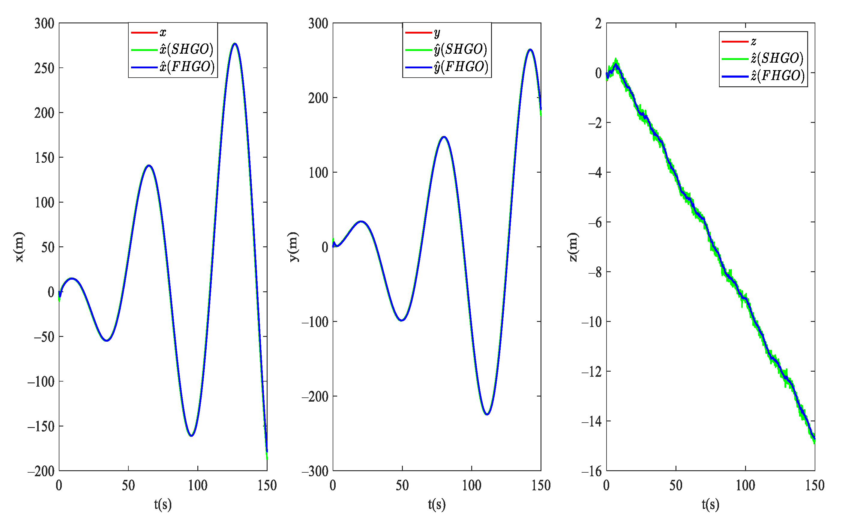
4.1. State Observer Simulation Result

To illustrate the noise resistance ability of the proposed FHGO, a simulation comparison is presented by applying the SHGO (20) in [29]. The design parameters are taken as $∍ = 0.05$, ${\partial }_1=4$, ${\partial }_2=4$. The low-pass filter is taken as

$$\frac{1}{T_f^2{s}^2+2T_{f}s+1}$$

$$A_f=\left[\begin{array}{cc}0& 1\\ -\frac{1}{T_f{}^2}& -\frac{2}{T_f}\end{array}\right],B_f=\left[\begin{array}{c}0\\ \frac{1}{T_f{}^2}\end{array}\right]$$

where $T_f=0.2$. The measurement noise ${\omega }_n$ is generated using the Simulink Band-Limited White Noise block with a noise power of 0.001 and sample time of 0.01 s. The following simulations in Figure 3, Figure 4 and Figure 5 illustrate the effectiveness of the filter in reducing the steady-state error and peak value in the beginning. We can find in Figure 4 and Figure 5 that the estimation of the SHGO observer is badly jittery, and the estimation of the FHGO is more stable.

4.2. Collision Avoidance Simulation Result

To show the performance of the controller of collision avoidance, we used the RBF neural network to estimate the unknown disturbance. Figure 6 shows that the UUVs follow the desired trajectory well and keep a good formation form. The distance between any two UUVs is more clear to show the collision. The $2r_c$ line is set at the bottom of Figure 7. If the distance $\Vert d_{ij}\Vert <2r_c$, collision occurs. Figure 7 shows the distance between any two UUVs of the formation considering collision avoidance. There is no line under the $2r_c$ line. The distance between UUVs is below to $2r_c$. With the collision avoidance control, the formation performance can be guaranteed.

The position error and velocity error performance are validated as shown in Figure 8. All the errors converge to zero in finite time, which means that the controller works satisfactorily and the system is stable. Simulation results show the four UUVs can track the virtual leader well without collision and maintain a good formation.

5. Conclusions

The adaptive neural network formation control for multi-UUVs with collision avoidance under unknown disturbance is discussed. Graph theory is utilized to model the communications between UUVs. Feedback linearization is used to simplify the 5-DOF mathematical model. The overall structure of the control law is composed of the formation controller and the collision avoidance controller. In the condition of unmeasurable states, FHGO is designed to exactly estimate the states of UUVs. The RBF neural network is adopted to approximate the nonlinear dynamic disturbance term. By integrating the artificial potential field method into the virtual leader-following formation strategy, the collision among UUVs problem is solved. The system stability is proven using the Lyapunov theory. The result shows the observer proposed in this paper performs better. Simulation results on formation control with collision avoidance demonstrated the controller designed in this paper is valid and performs well.

References

1. Zhou, K.-B.; Wu, X.-K.; Ge, M.-F.; Liang, C.-D.; Hu, B.-L. Neural-Adaptive Finite-Time Formation Tracking Control of Multiple Nonholonomic Agents with a Time-Varying Target. IEEE Access 2020, 8, 62943–62953. [Google Scholar] [CrossRef]
2. Li, X.; Wen, C.; Chen, C. Adaptive Formation Control of Networked Robotic Systems with Bearing-Only Measurements. IEEE Trans. Cybern. 2020, 51, 199–209. [Google Scholar] [CrossRef] [PubMed]
3. Brinon-Arranz, L.; Renzaglia, A.; Schenato, L. Multirobot Symmetric Formations for Gradient and Hessian Estimation with Application to Source Seeking. IEEE Trans. Robot. 2019, 35, 782–789. [Google Scholar] [CrossRef]
4. Park, B.S. Adaptive formation control of underactuated autonomous underwater vehicles. Ocean Eng. 2015, 96, 1–7. [Google Scholar] [CrossRef]
5. Wang, J.; Wang, C.; Wei, Y.; Zhang, C. Neuroadaptive Sliding Mode Formation Control of Autonomous Underwater Vehicles with Uncertain Dynamics. IEEE Syst. J. 2019, 14, 3325–3333. [Google Scholar] [CrossRef]
6. Gao, Z.; Guo, G. Fixed-time sliding mode formation control of AUVs based on a disturbance observer. IEEE/CAA J. Autom. Sin. 2020, 7, 539–545. [Google Scholar] [CrossRef]
7. Lu, Y.; Zhang, G.; Sun, Z.; Zhang, W. Robust adaptive formation control of underactuated autonomous surface vessels based on MLP and DOB. Nonlinear Dyn. 2018, 94, 503–519. [Google Scholar] [CrossRef]
8. Park, B.S.; Kwon, J.-W.; Kim, H. Neural network-based output feedback control for reference tracking of underactuated surface vessels. Automatica 2017, 77, 353–359. [Google Scholar] [CrossRef]
9. Franze, G.; Casavola, A.; Famularo, D.; Lucia, W. Distributed Receding Horizon Control of Constrained Networked Leader–Follower Formations Subject to Packet Dropouts. IEEE Trans. Control Syst. Technol. 2017, 26, 1798–1809. [Google Scholar] [CrossRef]
10. Astolfi, D.; Marconi, L.; Praly, L.; Teel, A. Sensitivity to High-Frequency Measurement Noise of Nonlinear High-Gain Observers. IFAC-PapersOnLine 2016, 49, 862–866. [Google Scholar] [CrossRef]
11. Khalil, H.K.; Priess, S. Analysis of the Use of Low-Pass Filters with High-Gain Observers. IFAC-PapersOnLine 2016, 49, 488–492. [Google Scholar] [CrossRef]
12. Abadi, A.S.S.; Hosseinabadi, P.A.; Mekhilef, S. Fuzzy Adaptive Fixed-time Sliding Mode Control with State Observer for A Class of High-order Mismatched Uncertain Systems. Int. J. Control. Autom. Syst. 2020, 18, 2492–2508. [Google Scholar] [CrossRef]
13. Prasov, A.A.; Khalil, H.K. A nonlinear high-gain observer for systems with measurement noise in a feedback control frame-work. IEEE Trans Autom Control 2013, 58, 569–580. [Google Scholar] [CrossRef]
14. Niu, B.; Duan, P.; Li, J.; Li, X. Adaptive Neural Tracking Control Scheme of Switched Stochastic Nonlinear Pure-Feedback Nonlower Triangular Systems. IEEE Trans. Syst. Man Cybern. Syst. 2019, 51, 975–986. [Google Scholar] [CrossRef]
15. Xu, N.; Zhao, X.; Zong, G.; Wang, Y. Adaptive control design for uncertain switched nonstrict-feedback nonlinear systems to achieve as-ymptotic tracking performance. Appl. Math. Comput. 2021, 408, 126344. [Google Scholar]
16. Ma, L.; Xu, N.; Zhao, X.; Zong, G.; Huo, X. Small-Gain Technique-Based Adaptive Neural Output-Feedback Fault-Tolerant Control of Switched Nonlinear Systems with Unmodeled Dynamics. IEEE Trans. Syst. Man Cybern. Syst. 2020, 51, 7051–7062. [Google Scholar] [CrossRef]
17. Sakai, D.; Fukushima, H.; Matsuno, F. Leader–Follower Navigation in Obstacle Environments While Preserving Connectivity without Data Transmission. IEEE Trans. Control Syst. Technol. 2017, 26, 1233–1248. [Google Scholar] [CrossRef] [Green Version]
18. Dong, Y.; Su, Y.; Liu, Y.; Xu, S. An internal model approach for multi-agent rendezvous and connectivity preservation with nonlinear dynamics. Automatica 2018, 89, 300–307. [Google Scholar] [CrossRef]
19. Wen, G.; Chen, C.L.P.; Liu, Y.-J. Formation Control with Obstacle Avoidance for a Class of Stochastic Multiagent Systems. IEEE Trans. Ind. Electron. 2017, 65, 5847–5855. [Google Scholar] [CrossRef]
20. Park, B.S.; Yoo, S.J. An Error Transformation Approach for Connectivity-Preserving and Collision-Avoiding Formation Tracking of Networked Uncertain Underactuated Surface Vessels. IEEE Trans. Cybern. 2018, 49, 2955–2966. [Google Scholar] [CrossRef]
21. Zhong, H.; Wang, Y.; Miao, Z.; Tan, J.; Li, L.; Zhang, H.; Fierro, R. Circumnavigation of a Moving Target in 3D by Multi-agent Systems with Collision Avoidance: An Orthogonal Vector Fields-based Approach. Int. J. Control. Autom. Syst. 2019, 17, 212–224. [Google Scholar] [CrossRef]
22. He, S.; Wang, M.; Dai, S.-L.; Luo, F. Leader–Follower Formation Control of USVs with Prescribed Performance and Collision Avoidance. IEEE Trans. Ind. Inform. 2018, 15, 572–581. [Google Scholar] [CrossRef]
23. Huang, Y.; Liu, W.; Li, B.; Yang, Y.; Xiao, B. Finite-time formation tracking control with collision avoidance for quadrotor UAVs. J. Frankl. Inst. 2020, 357, 4034–4058. [Google Scholar] [CrossRef]
24. Fossen, T.I. Handbook of Marine Craft Hydrodynamics and Motion Control; John Wiley & Sons: Hoboken, NJ, USA, 2011. [Google Scholar]
25. Yan, Z.-P.; Liu, Y.-B.; Yu, C.-B.; Zhou, J.-J. Leader-following coordination of multiple UUVs formation under two independent topologies and time-varying delays. J. Cent. South Univ. 2017, 24, 382–393. [Google Scholar] [CrossRef]
26. Shi, Q.; Li, T.; Li, J.; Chen, C.P.; Xiao, Y.; Shan, Q. Adaptive leader-following formation control with collision avoidance for a class of second-order nonlinear multi-agent systems. Neurocomputing 2019, 350, 282–290. [Google Scholar] [CrossRef]
27. Wen, G.; Chen, C.L.P.; Dou, H.; Yang, H.; Liu, C. Formation control with obstacle avoidance of second-order multi-agent systems under directed communication topology. Sci. China Inf. Sci. 2019, 62, 192205. [Google Scholar] [CrossRef] [Green Version]
28. Khalil, H.K.; Praly, L. High-gain observers in nonlinear feedback control. Int. J. Robust Nonlinear Control 2014, 24, 993–1015. [Google Scholar] [CrossRef]
29. Pang, Z.H.; Zheng, C.B.; Sun, J.; Han, Q.L.; Liu, G.P. Distance- and velocity-based collision avoidance for time-varying formation control of sec-ond-order multi-agent systems. IEEE Trans. Circuits Syst. II Express Briefs 2021, 68, 1253–1257. [Google Scholar] [CrossRef]
Figure 1. Coordinate system of a UUV.
Electronics 11 01170 g001
Figure 2. Collision sphere and the collision avoidance sphere of UUVs.
Electronics 11 01170 g002
Figure 3. Position states estimation of state observer in x, y and z directions.
Electronics 11 01170 g003
Figure 4. Velocity state estimation of state observer.
Electronics 11 01170 g004
Figure 5. Angle velocity state estimation of state observer.
Electronics 11 01170 g005
Figure 6. Three-dimensional (3D) trajectory of the UUV formation with collision avoidance under unknown disturbance.
Electronics 11 01170 g006
Figure 7. Distance between any two UUVs of the formation with collision avoidance.
Electronics 11 01170 g007
Figure 8. Position errors and velocity errors of UUVs.
Electronics 11 01170 g008