1. Introduction
Assessing the quality of Target Recognition Video (TRV) is different from assessing the quality of entertainment video. Given the use of TRV, the qualitative assessment does not focus on the subject’s satisfaction with the quality of the video sequence, but measures how the subject uses TRV to perform specific tasks [
1]. These tasks may include: Video surveillance—recognising number plates, telemedicine/remote diagnostics—correct diagnosis, fire safety—fire detection, rear-view cameras—parking the car, gaming—recognising and correctly responding to a virtual enemy, video messaging and report generation—video summarisation [
2,
3]. In relation to entertainment videos, research has been conducted on the content parameters that most influence perceptual quality. These parameters provide a framework for creating predictors and thus developing objective measures through the use of subjective tests. However, this framework is not suitable for recognition tasks. Therefore, one has to develop new ones. The problem is not limited to the methods for testing the quality of a video. The conditions for when and how the video is recorded are also crucial. One has to take into account the exposure, ISO, visual acuity, bit rate, and many more to conduct a valid experiment.
Historically, any assessment of quality has been made by subjective methods, i.e., by conducting psycho-physical experiments with subjects. The co-authors of this paper have also been involved in such work, resulting in, among other things, the specific ITU-T Recommendation [
4]. However, such an assessment is very tedious and time-consuming. Therefore, there is a tendency to replace psycho-physical experiments with quality modelling metrics. Nowadays, there are many metrics for general Quality of Experience (QoE), both those with Full-Reference (FR), such as Peak Signal-to-Noise Ratio—PSNR or Structural Similarity—SSIM, and those with No-Reference (NR), such as Video Quality Indicators (VQI), which are successfully used in video processing systems to evaluate entertainment video quality. However, they are not suitable when dealing with video sequences used for recognition tasks (TRV). Therefore, correctly estimating the performance of video processing pipelines is still a major challenge for researchers, both in manual and Computer Vision (CV) recognition tasks. There is a need for an objective method to evaluate video quality for recognition tasks.
Such an objective method of assessing video quality for recognition tasks can have very practical applications. For example, usually, the smart car Neural Network (NN) algorithms are trained on high-quality data captured in ideal conditions. An actual car on the road might need to drive in a wide range of less-than-ideal conditions, and it is hard to predict how that would influence the output of the network. To prevent catastrophic failures, we would like to trigger a warning to the driver when the input quality is not sufficient for adequate NN performance. In response to this need, in this work, we develop and test a critical element of a system that can predict machine vision performance based on the quality of the input stream. More specifically, the objective of this paper is to show that it is possible to achieve an accurate model that estimates the performance of TRV processing pipelines. As contributions of this paper, we:
Collect a representative set of image sequences—based on the subset of the “Labelled Faces in the Wild (LFW)” database [
5,
6,
7,
8] (addressed in
Section 2.1);
Set a series of degradation scenarios based on the model of the digital camera and how the luminous flux reflected from the scene will eventually become a digital image (addressed in
Section 2.2);
Evaluate the resulting degraded images using a face recognition CV library—based on the state-of-the-art Deep Learning dlib software library (addressed in
Section 2.3) as well as VQI—eleven (11) of which are from our AGH Video Quality (VQ) team and another eight (8) from external labs (addressed in
Section 2.4);
Develop a new concept for an objective model to evaluate video quality for face recognition tasks (addressed in
Section 3);
Train, test, and validate the model (addressed in
Section 3);
Show that it is possible to achieve a measure of model accuracy, expressed as the value of the F-measure parameter, of 0.87 (addressed in
Section 3).
It is worth emphasising at this point how different our work is from the most recent work of others in this field. Shi et al. [
9] propose an innovative video quality assessment method and dataset for impaired videos. This work relates to TRV, but the data modality differs significantly from our case. While we focus on face recognition tasks, Shi et al. (this work is a winner of the NIST Enhancing Computer Vision for Public Safety Challenge Prize) focus on public safety. Similarly, Xing et al. [
10] address a seemingly similar area (TRV), but focus on the detection and classification of individual fusion traces (process windows in selective laser melting). Another area where a lot of research is being done on TRV quality assessment is laparoscopic images. A relatively recent example is a paper published by Khan et al. [
11]. Hofbauer et al. [
12] publish a database of encrypted images with subjective recognition ground truth. The reported research is from a similar domain as ours, but only concerns distortions in image encryption. Wu et al. [
13] propose a continuous blind (NR) prediction of image quality with a cascaded deep neural network. The deep Convolutional Neural Network (CNN) used has achieved great success in assessing the quality of image recognition. However, Wu et al. express quality using Mean Opinion Score (MOS) but do not measure how the subject uses TRV to perform specific tasks. A similar approach is presented by Oszust [
14], who proposes a local feature descriptor and derived filters for blind (NR) assessment of image quality, and by Mahankali [
15], who presents NR assessment of video quality using voxel-wise fMRI models of the visual cortex. Finally, it is worth recalling here a review of recent methods for objective assessment of video quality in recognition tasks, which we presented in [
16]. This discusses older related solutions developed by different research teams.
The rest of this paper is as follows:
Section 2 presents the required experimental research plan.
Section 2.1 includes the preparation of a corpus of Source Reference Circuits (SRC), which are original video sequences consisting of preexisting footage.
Section 2.2 involves the preparation of a set of Hypothetical Reference Circuits (HRC), which are different scenarios of video degradation.
Section 2.3 and
Section 2.4 include the experiment that generates two sets of data: recognition data and quality data, respectively. Since we have two sets of data (from the recognition experiment and the quality experiment), we can build a model that predicts the recognition results based on video quality indicators. The results are reported in
Section 3.
Section 4 concludes this work.
2. Materials & Methods
This section presents a general description of the research. The experiment contains one source data set (Source Reference Circuits—SRCs,
Section 2.1) and a couple of distortion types (Hypothetical Reference Circuits—HRCs,
Section 2.2). One impairs each SRC with each of the HRCs. The resulting sequences are evaluated using a face recognition computer vision library (
Section 2.3) and VQI (
Section 2.4).
2.1. Acquisition of the Existing Source Reference Circuits (SRC)
This subsection introduces the customised dataset for this study; thus, it contains a technical description on the selected SRCs. A corpus of original SRC video sequences consists of already available footage.
The SRC database comprises several selected video frames. The selection criterion was to establish a database that covers as many different features as possible. In the following, we have provided the description of the data set.
We used only the subset of the entire SRC set for the experiment. However, the first step to select a subset of SRC is to determine the size of that subset. For this purpose, the underlying assumption is made that one training experiment, one subsequent optional training experiment, and one testing experiment (model validation) are carried out. We arbitrarily agree that the first and second training experiments have sets of equal numbers of elements, while the test set has several elements equal to a quarter of the size of a single training experiment.
Another assumption is that (for practical reasons) a single experiment iteration cannot last more than a week. This assumption has a de facto impact only on the number of elements of the training set—test sets are four times smaller.
At this point, it is worth noting that the processing time of a single image decisively influences the number of images used in each experiment. This time consists of the sum of image processing in the two components of the experiment, the Recognition Experiment (
Section 2.3) and the Quality Experiment (
Section 2.4). Knowing the average time needed to perform the Quality Experiment for one image and knowing the average time needed to perform the Recognition Experiment for one image, we are able to estimate the number of images that can be processed per week, i.e., the number of images that can be used in one experiment iteration.
It is also worth noting that, of course, the number specified by the above method does not specify the number of usable SRC images but the number of usable Processed Video Sequence (PVS) images. To know the number of usable SRC images, we divide the number of usable PVS images by the number of HRC defined. The number of HRCs is 64 (+1 SRC).
To move on to specific values, one determines that the average processing time of one image in the Quality Experiment is relatively long and amounts to the order of magnitude of hundreds of seconds. The average image processing time in the Recognition Experiment is below one second, so it is relatively negligible.
What results from the above is that, during the week, PVS images based on 120 SRC images can be processed, which, therefore, results in the preparation of 80 SRC images for the training experiment, a further 20 (quarter) SRC images for the test experiment, and a further 20 (quarter) SRC images for the validation. Each SRC image contains one object (face) to be recognised. In total, 120 objects are detected.
As mentioned before, a validation set is prepared, but temporarily put aside without processing. The size of this set is equal to the size of the corresponding test set.
The remainder of this subsection presents the complete set (
Section 2.1.1) and the subset selected for the experiment (
Section 2.1.2).
2.1.1. The Face Recognition Set
The source of the full data set for Face Recognition is the Labeled Faces in the Wild (LFW) database [
5,
6,
7,
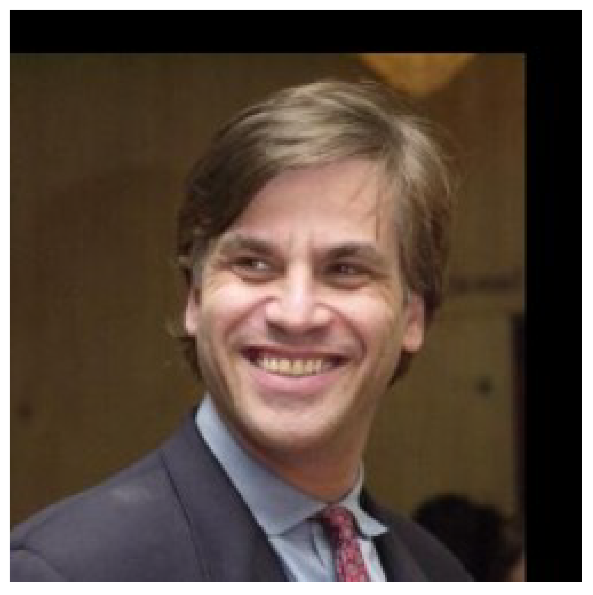
8]. LFW is a public benchmark for face verification, also known as pair matching. LFW is a database of face photographs designed to study the problem of unconstrained face recognition. The data set contains 13,233 images of the faces of 5749 different people collected from the Web. Each face has a resolution of 250 × 250 and is labelled with the name of the person pictured. In addition, 1680 of the people pictured have two or more distinct photos in the data set. The only constraint on these faces is that they were detected by the Viola–Jones face detector.
Figure 1 presents the selected SRC frame.
In terms of the dataset, the LFW photos are already in JPEG format. We ensure that they are all of equal initial quality by visual assessment because they came from a variety of sources. Furthermore, we ensure that the face recognition system (discussed in greater detail in
Section 2.3.2) can easily recognise faces in the LFW photos.
2.1.2. The Face Recognition Subset
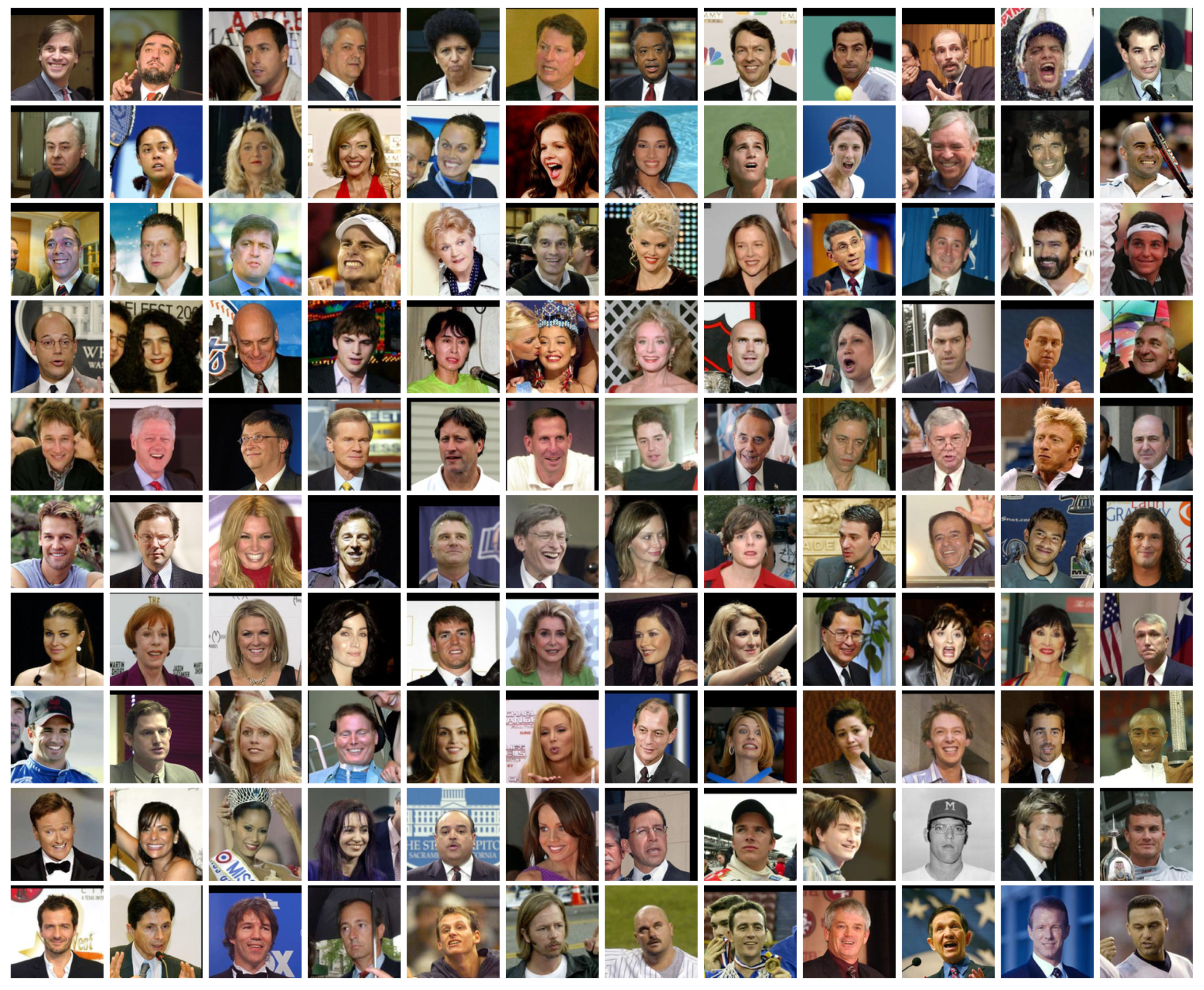
The whole set is subsampled, which results in 120 images divided into a training set, a test set, and a validation set—in a ratio of 80 vs. 20 vs. 20, respectively.
Figure 2 presents the montage of selected SRC frames for face recognition.
2.2. Preparation of Hypothetical Reference Circuits (HRC)
This subsection describes the degradation scenarios (i.e., Hypothetical Reference Circuits or HRCs). The proposed set of HRCs contains a range of distortions related to the whole digital image acquisition pipeline. Importantly, the selection of HRCs defines the applicability of the quality evaluation method proposed in this paper.
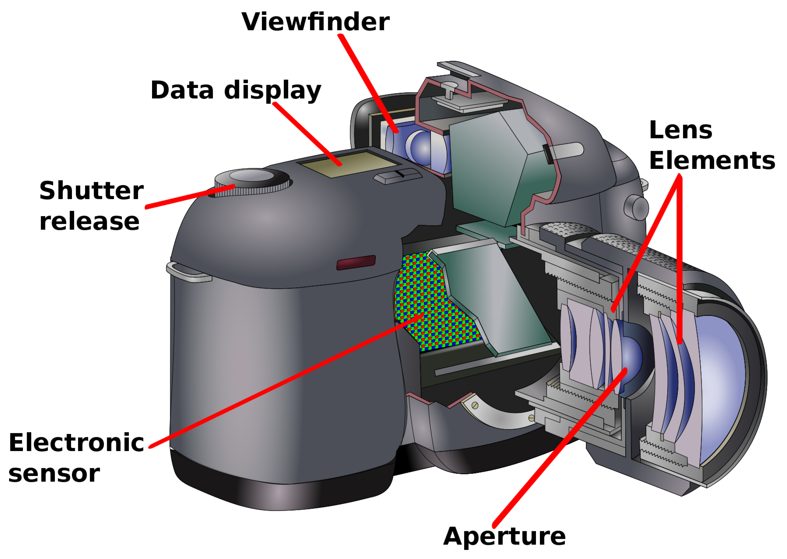
The HRC set is based on the digital camera model (see
Figure 3) and how the luminous flux reflected from the scene eventually becomes a digital image. Light, before it reaches the lens elements, may be already weakened, e.g., by improper exposure to photographic lighting. The light beam may move through out-of-focus lens elements, and the aperture can cause blur (defocus aberration). Then, the luminous flux falls on an electronic sensor that has a finite resolution. Further stages of analog-to-digital conversion and signal amplification may again be the source of Gaussian noise. Moreover, it may turn out that, due to prolonged exposure time, the motion blur effect may appear. In the final processing step, artefacts may result from JPEG compression.
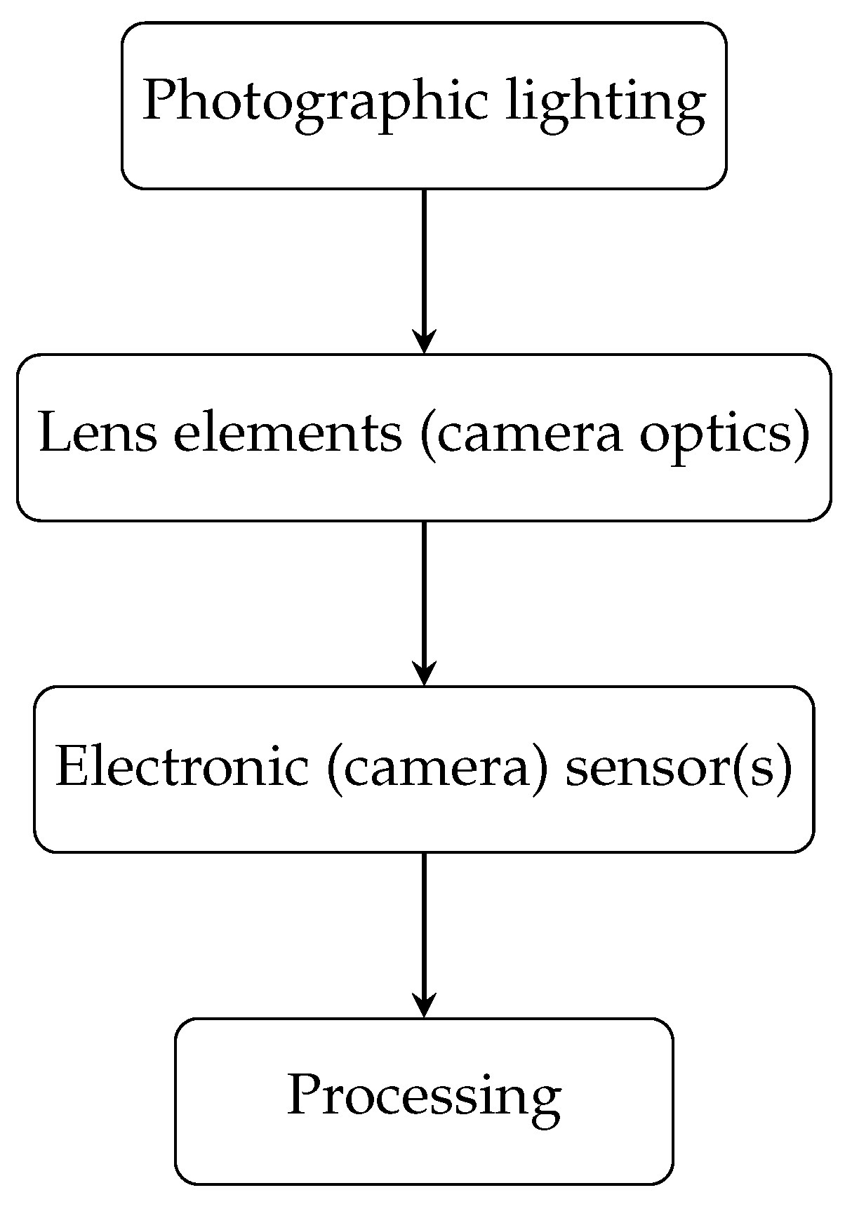
The distortion model is shown in
Figure 4.
We select the following HRCs:
HRC related to photographic lighting:
- (1)
Image under/overexposure;
HRC related to lens elements (camera optics):
- (2)
Defocus (blur);
HRC related to electronic (camera) sensor(s):
- (3)
Gaussian noise;
- (4)
Motion blur;
HRC related to processing:
- (5)
JPEG compression.
We decide to use FFmpeg [
17] and ImageMagick [
18] as tools for applying HRCs. They already incorporate a set of relevant filters. We use them to generate all distortions. The former tool is used to apply the image under/overexposure and Gaussian noise. The latter tool is used to apply the defocus distortion, simulate the motion blur degradation, and perform JPEG compression.
One measures the tools’ computation performance for the extreme case (enabling all filters), obtaining a result of 439 frames per minute. One performs this test on a standard laptop (Intel i5—3317U and 16 GB of RAM).
Table 1 presents the thresholds for specific distortions (listed in rows). Usually, they are determined so that the place (HRC value) for which there is zero recognition is determined (this place is the penultimate step; for safety, we include one more step). The steps are linear.
Table 2 shows distortions. Additionally, for each type of distortion, the expected number of distortion intensity levels is given. As one can see, there are six levels for most of these distortions. The exception is exposure (which, due to its bidirectional nature, requires twice as many levels of distortion) and JPEG. Moreover, in the case of a combination of distortions (last three rows in the table, forming a separate subsection), there are only five levels, since we generate the extreme levels already when generating single distortions (previous subsection in the table).
In the case of a combination of distortions, the order in which they are applied is important:
For Motion Blur + Gaussian Noise, we apply Motion Blur first.
For Over-Exposure + Gaussian Noise, we apply Over-Exposure first.
For Under-Exposure + Motion Blur, we apply Motion Blur first (however, the more appropriate order should be: Under-Exposure first, but we reversed the order for technical reasons caused by possible interpolation problems).
Of course, one more “distortion” should be added to the number of distortions, which is “no distortion” (pure SRC). To sum up, there are 64 HRC variants (+1 SRC).
Having SRC prepared and HRC defined, the actual video processing can occur, preparing a corpus of Processed Video Sequences—PVS—being SRC images distorted using HRC degradation scenarios. The expected result is a PVS corpus.
In the following, detailed information on distortions and their application is provided.
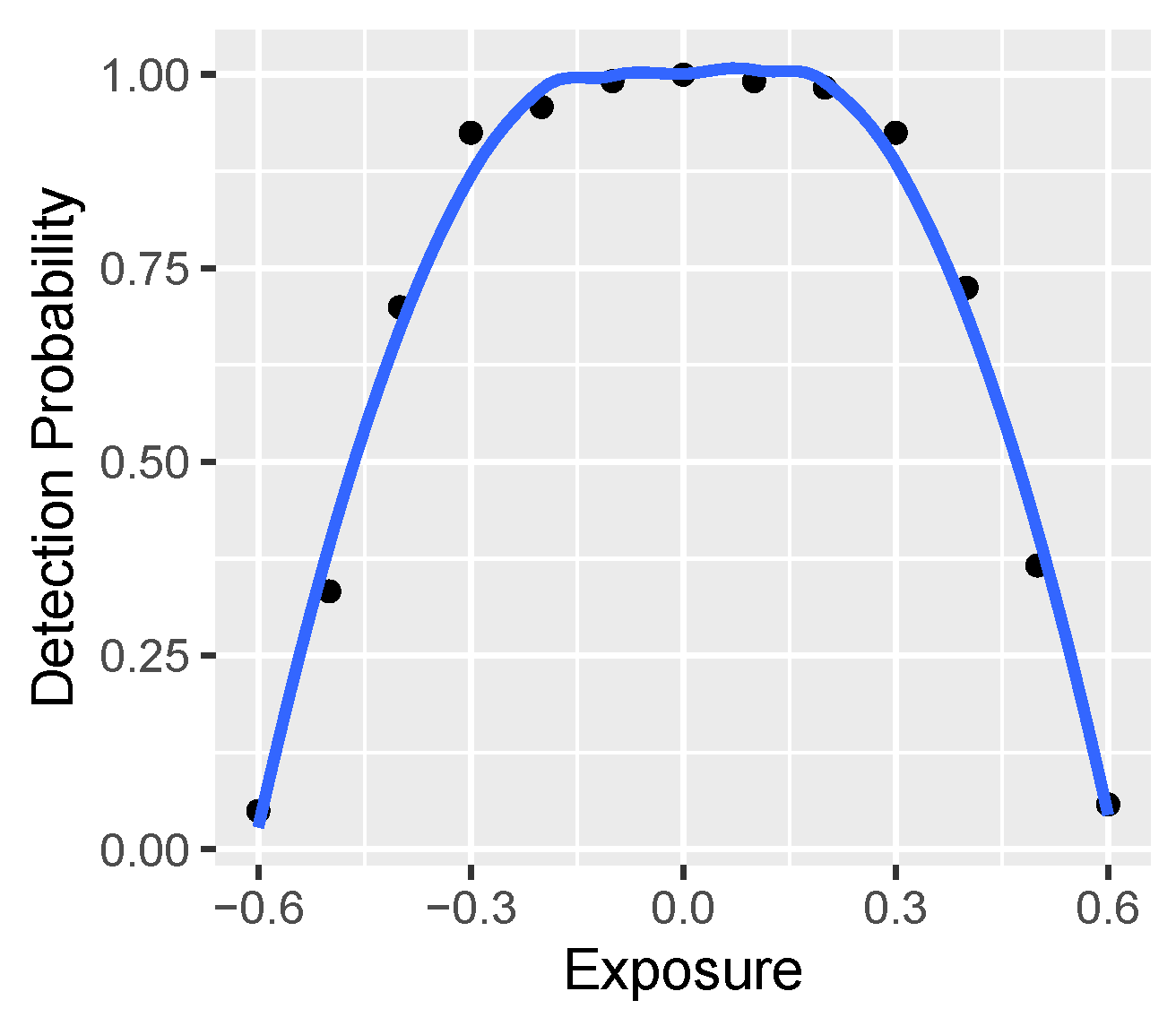
2.2.1. Exposure (Photography)
Exposure in photography is the amount of light that falls on light-sensitive materials such as photopaper or electrical sensors. It is one of the most critical parameters while taking a frame. Its value is determined by the shutter speed and lens aperture ratio with the chosen ISO. Exposure is measured in (fractions of) seconds while the aperture is open. In case of too much light, the frame is overexposed. On the other hand, too little light can cause an underexposed scene [
19].
In our HRC generation tool, to modify the exposure, the FFmpeg equaliser (“eq”) filter is used. This filter enables setting brightness, contrast, saturation, and approximate gamma adjustments. The full set of acceptable options is available on
https://ffmpeg.org/ffmpeg-filters.html#eq, accessed on 31 December 2021.
Overexposed images lead to white, unrecognisable faces. On the other hand, underexposed images create dark spots in the image. The information contained in the highlighted or black part of the image is irrecoverable.
The overexposure and underexposure generated in such a way successfully meet the requirements. FFmpeg filter allows modifying an exposure in a wide range. It allows us to create HRCs ready to test the performance of face recognition system as a method of face recognition. The border exposure value makes it impossible for a human to recognise the face. Hence, HRC covers the whole visible scope.
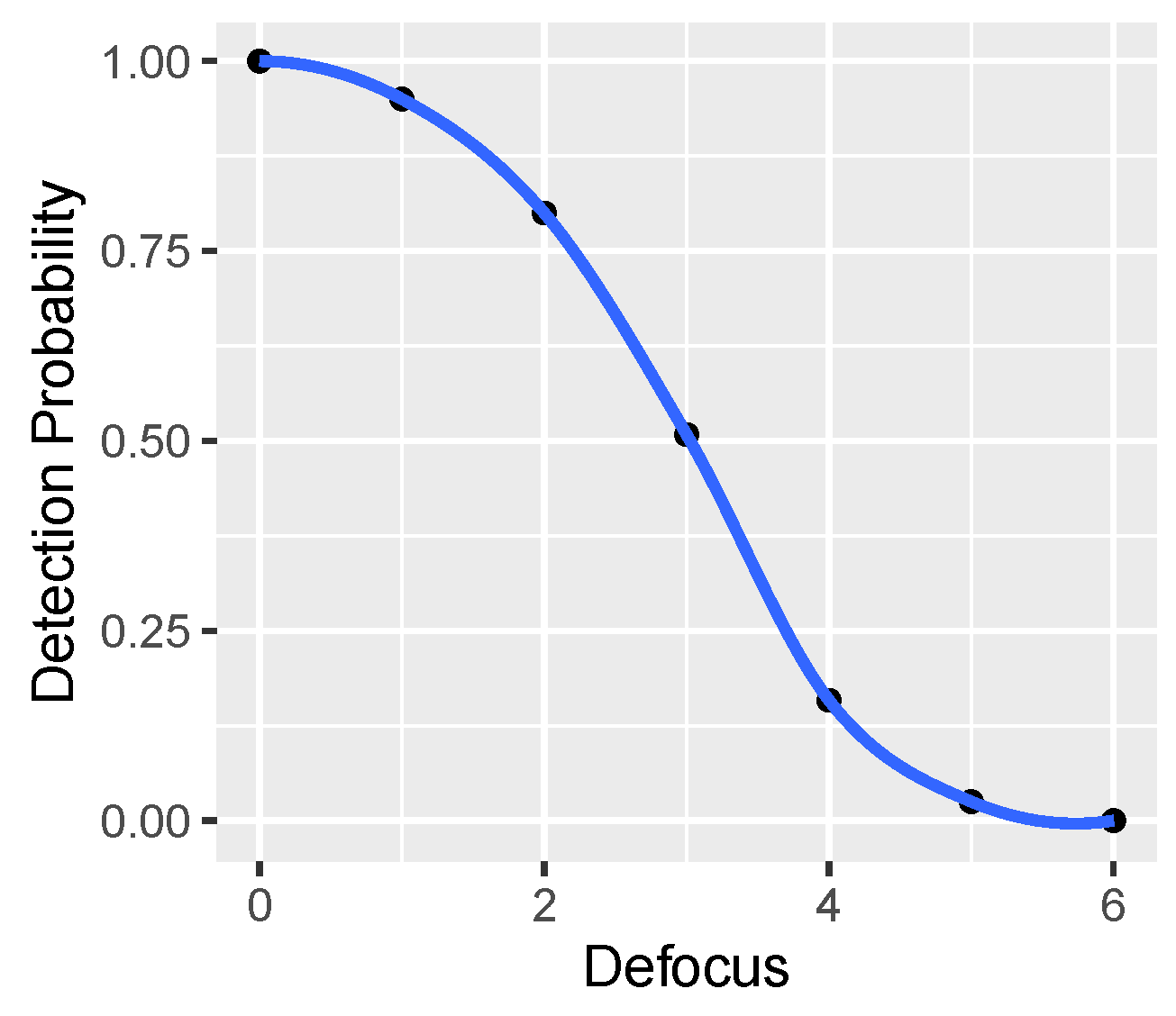
2.2.2. Defocus
Defocus is a distortion in which the image is out of focus. Is it an aberration that appears in every device equipped with a lens like a camera, video camera, telescope, or microscope. Defocus diminishes the contrast of the image and object sharpness. It means that sharp high-contrasted edges become blurry and finally unrecognisable. On the other hand, making the image too sharp leads to a grain effect visible in the image. In general, maximising image quality is doable by minimising defocus [
20].
In this case, one can set a sigma value. One could understand sigma as an approximation of just how much the image pixels should be “spread” or blurred. The radius parameter is set to 0, as recommended in the documentation.
The ImageMagick allows one to create the proper defocus degradation. In other words, we are able to apply this technique to a fine-grained step. Notice that even a small sigma parameter (used to control the distortion strength) creates frames in which the face is impossible to recognise. Hence, the proper step has to be applied when generating PVSs. Failure to do so may result in a too rapid degradation of the source content.
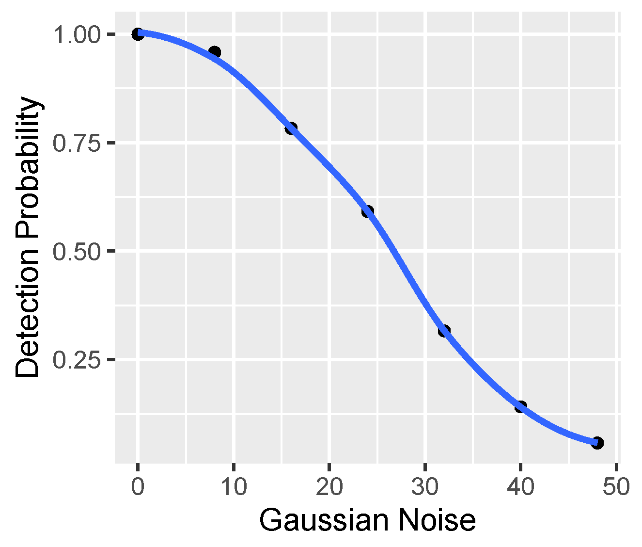
2.2.3. Gaussian Noise
Gaussian noise is also known as statistical noise. Its most prominent feature is that the probability density function is equal to the normal distribution. The only values that noise can have are Gaussian-distributed [
21].
All cameras have an automatic denoising algorithm. We do not want to apply a noise standalone, but to keep it as realistic as possible. Consequently, we model it by first applying noise and immediately after denoising the frame.
To generate this distortion, we use the “noise” FFmpeg filter
https://ffmpeg.org/ffmpeg-filters.html#noise, accessed on 31 December 2021). We set the noise strength for a specific pixel component. Additionally, “bm3d” FFmpeg filter (
https://ffmpeg.org/ffmpeg-filters.html#bm3d, accessed on 31 December 2021) MDPI: please add acess date (day month year). is used to prevent using raw noise. This filter denoises frames using the Block-Matching 3D algorithm. In our scenario, a sigma (denoising strength) is specified as equal to the noise value. However, this value should be adjusted according to the source, as Block-Matching 3D algorithm is susceptible to sigma. Local patch sets (blocks), the sliding step for processing blocks, and a maximal number of similar blocks in the third dimension are hard-coded. The simple conclusion is that the higher the noise value, the more disturbed is the image, and the recognition task is harder to perform.
The maximum value of noise outputs the frame, where a human cannot recognise faces. Consequently, we consider HRCs produced using this filter to be appropriate for testing a recognition algorithm.
2.2.4. Motion Blur
Motion blur is seen only in sequence with moving objects as a motion streak. It is observable when the recorded object changes position. Motion blur can be caused by rapid object movement combined with long shoot exposure [
22].
As a tool to create a motion blur degradation, we choose ImageMagick. We decide to use radial blur, which allows for blurring of the image in a circle. It creates an effect as the image spins around. This filter requires an argument, which is the angle that the radial blur covers. Documentation (
http://www.imagemagick.org/Usage/blur/#radial-blur, accessed on 31 December 2021) shows the results of different angle values.
Motion blur is the most demanding degradation. To obtain the best results for motion blur degradation, ImageMagick filters are the best option.
2.2.5. JPEG
JPEG is the most popular image compression standard and digital image format in the world. Several billion JPEG images are produced every day, particularly through digital photography. JPEG is largely responsible for the proliferation of digital images across the Internet and later in social networks. JPEG employs lossy compression. The compressor can achieve higher compression ratios (i.e., smaller file sizes) at the cost of image quality. JPEG typically achieves 10:1 compression with little perceptible quality loss. JPEG uses an 8 × 8 discrete cosine transform (DCT), a zigzag scan of the transform coefficients, Differential Pulse-Code Modulation (DPCM), prediction of average block values, scalar quantisation and entropy coding. Entropy coding typically uses Huffman-style variable length codes, but an arithmetic coding option (more efficient and processing-intensive) is also available in the standard [
23].
2.3. Recognition Experiment
This subsection describes the setup of the recognition experiment. Its first subsection (
Section 2.3.1) provides a general overview. The second one (
Section 2.3.2) details the face recognition system used. The last subsection (
Section 2.3.3) discusses the face recognition execution time.
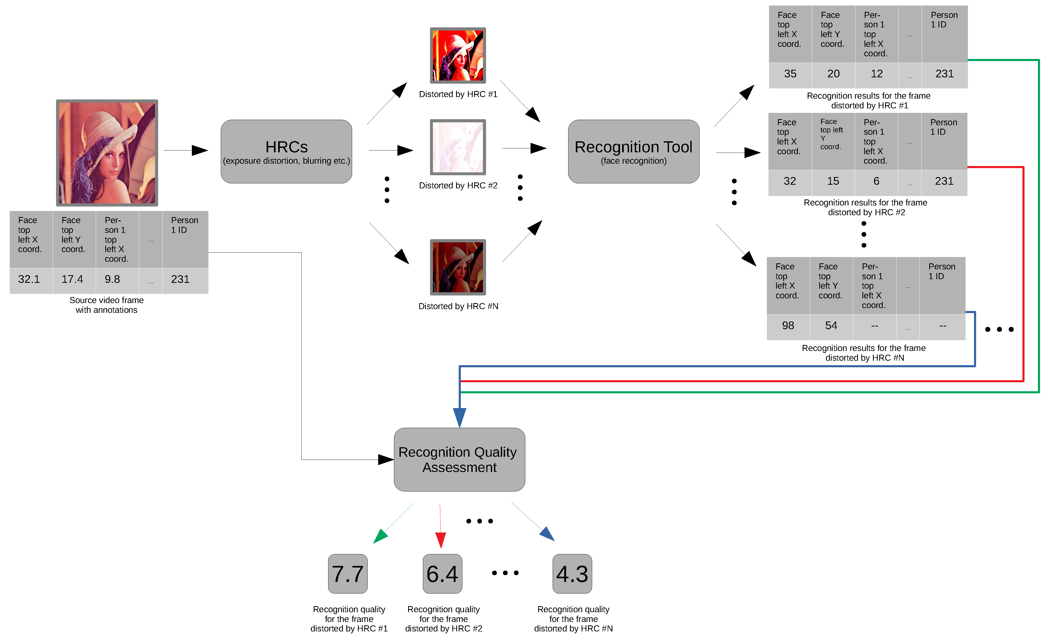
2.3.1. Recognition Experiment Overview
Each of the obtained PVS is a single frame. For such a frame, we use a face recognition system.
Figure 5 presents a general processing pipeline that we use in the recognition experiment.
2.3.2. Face Recognition System
Face recognition is based on a state-of-the-art deep learning dlib software library (
https://github.com/ageitgey/face_recognition, accessed on 31 December 2021). The library analyses pictures to detect faces and to compare the encoding of recognised faces with newly detected encoding of the faces. The algorithm works with all types of images. With an additional function, it is possible to work with video files. The function performs the task of dividing the video into single frames. Next, every frame is subject to detection and recognition. Finally, the algorithm returns all detected and recognised known faces and all not recognised faces. Moreover, there is another additional function to return the coordinates of all detected faces on the image. The model has an accuracy above 93%.
The system is simple to use in recognising faces on the image. To increase the probability of recognition, we teach the system with as many pictures of each known person as possible.
2.3.3. Face Recognition Execution Time
As we mentioned earlier, to be able to assess how many SRCs we can test, we need to know how long all face recognition processes take to compute. The average execution time of the face recognition computer vision algorithm per single video frame is 0.068 s. Importantly, execution times are assessed using a PC with Intel Core i5-8600K CPU.
2.4. Quality Experiment
This subsection describes the setup of the quality experiment. Its first subsection (
Section 2.4.1) provides a general overview. The second one (
Section 2.4.2) details what Video Quality Indicators (VQIs) are used. Subsection (
Section 2.4.3) discusses the VQI execution time. The last subsection (
Section 2.4.4) shows the sample data.
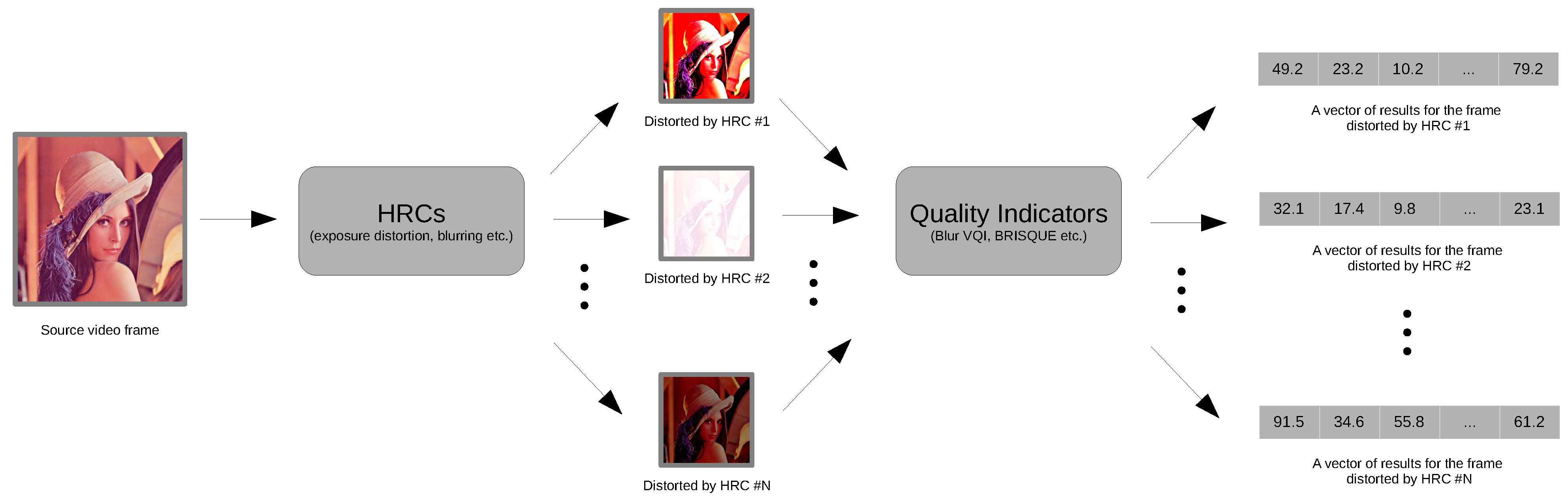
2.4.1. Quality Experiment Overview
The experiment operates on individual video frames (with one exception of Temporal Activity VQI). It applies a set of VQIs and outputs a vector of results (one for each VQI.
Figure 14 presents a flowchart of this process. The results will be combined later with those from the recognition experiment. Together, they will constitute input data for modelling.
Depending on the VQI, we use either C/C++ or MATLAB code.
2.4.2. Indicators
In total, we are using 20 VQIs. Eleven (11) of them come from our AGH Video Quality (VQ) team. Another eight (8) come from external laboratories.
Table 3 lists all VQIs, along with their descriptions. It also includes references to related publications. Indicators marked with an asterisk (*) are not directly in line with the scope of the project. Nevertheless, we include them as they may prove significant (at the modelling stage) and do not add much computation time overhead. UMIACS stands for the University of Maryland Institute for Advanced Computer Studies (Language and Media Processing Laboratory); BUPT stands for Beijing University of Posts and Telecommunications (School of Information and Communication Engineering).
When preparing for the experiment, we reject two indicators: (i) DIIVINE [
37] and (ii) BLIINDS-II [
38]. Both of them show long computational times (with BLIINDS-II taking around 3 min to evaluate the quality of an image). Rejecting DIIVINE and BLIINDS-II is necessary to keep the experiment meaningful in terms of the number of SRCs utilised. In other words, incorporating DIIVINE and BLIINDS-II makes the experiment execution so slow that we are not being able to test a sufficiently high number of SRCs.
We decide to discard DIIVINE at the same time providing a solution resulting from it. Specifically, we expect FFRIQUEE to be at least as good as DIIVINE. This is because FRIQUEE builds on top of DIIVINE.
On the other hand, there is no replacement indicator for BLIINDS-II. We reject it because of the possibility that this indicator performs better than others. However, based on the existing works [
39], we do not anticipate that this indicator would prove to be a top-performing one.
2.4.3. VQI Execution Time
As we mentioned before, to be able to assess how many SRCs we can test, we need to know how long all VQIs take to compute.
Table 4 presents execution times of all VQIs. Importantly, the execution times are assessed using a laptop with an Intel Core i7-3537U CPU.
2.4.4. Example Data
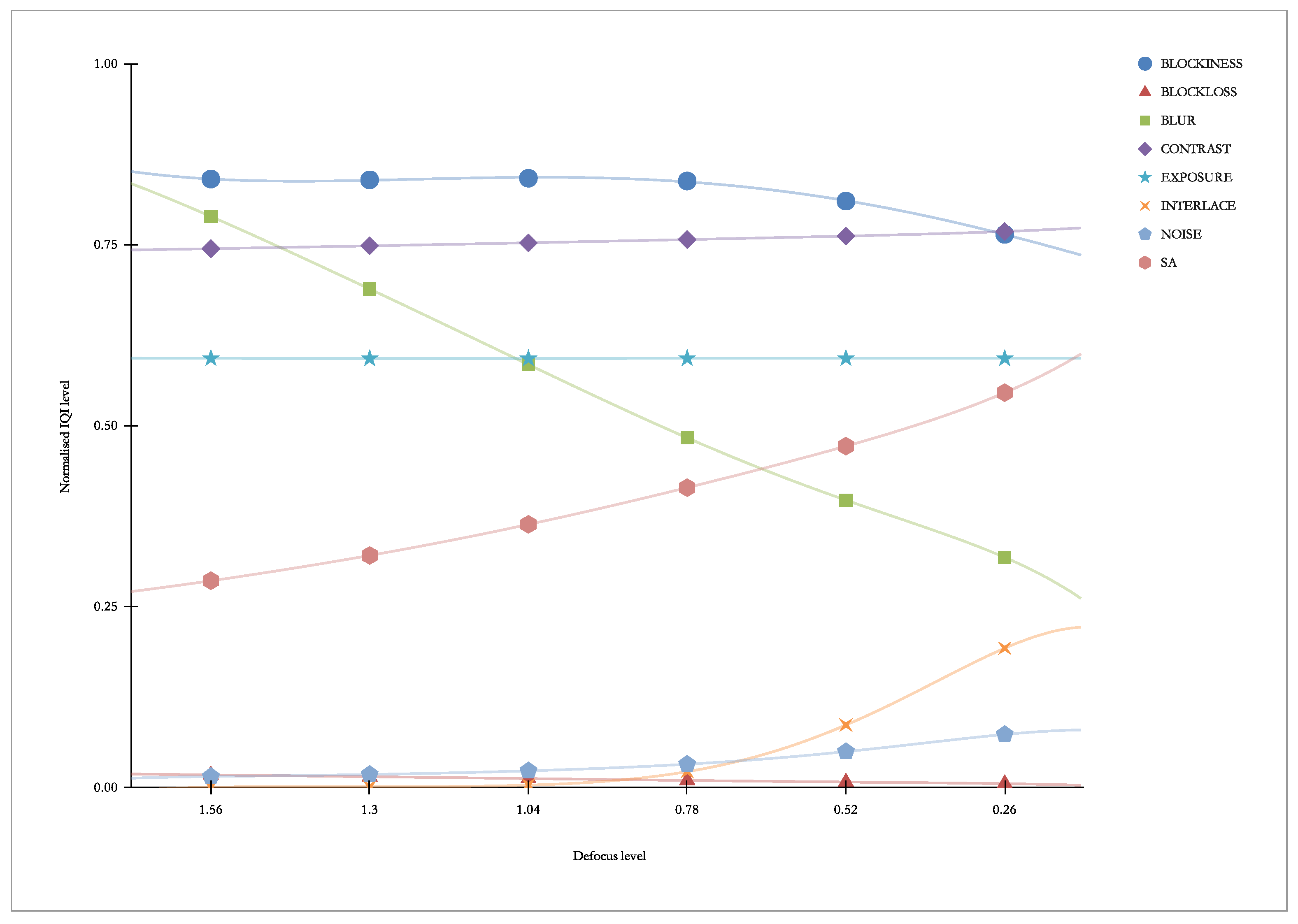
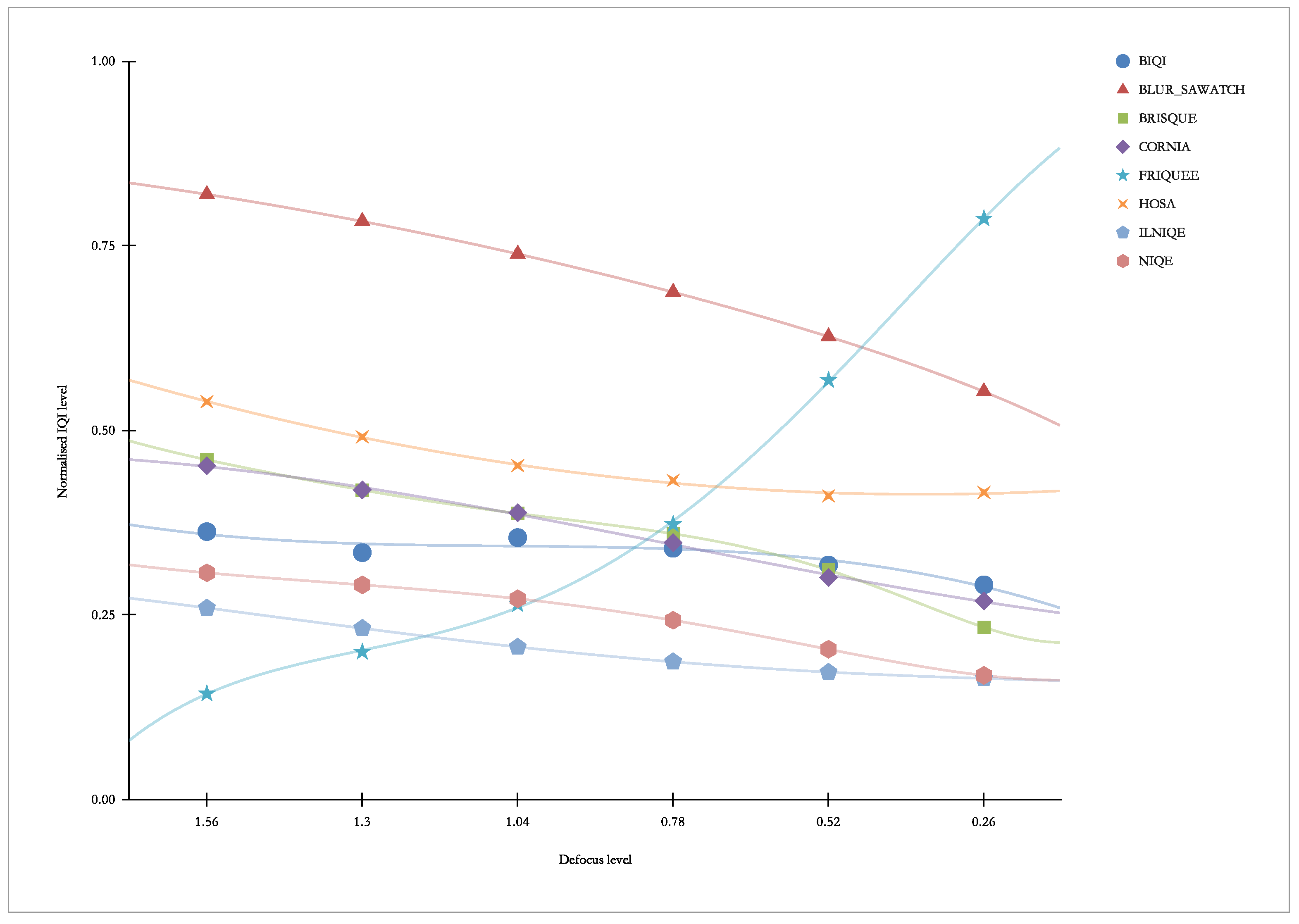
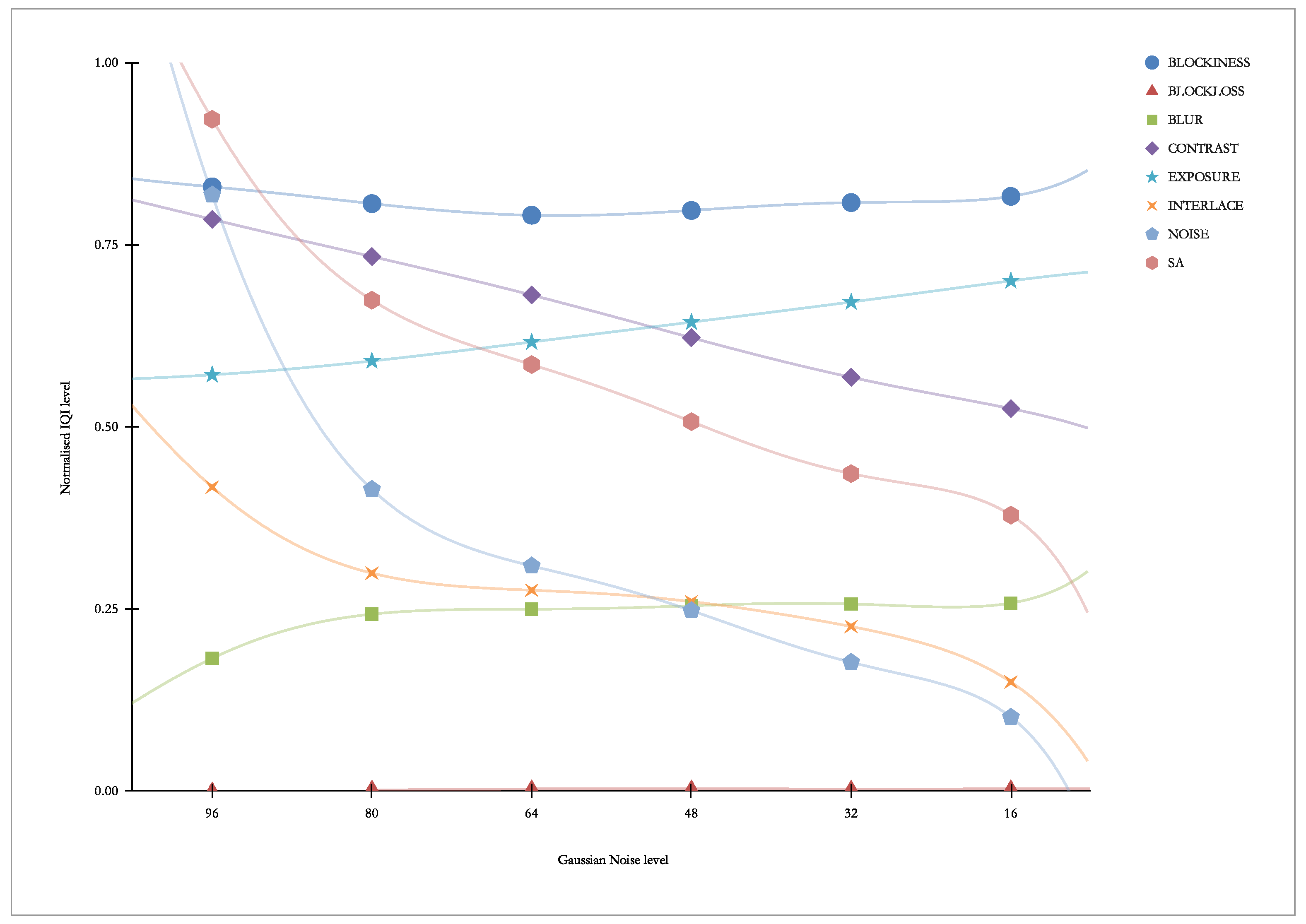
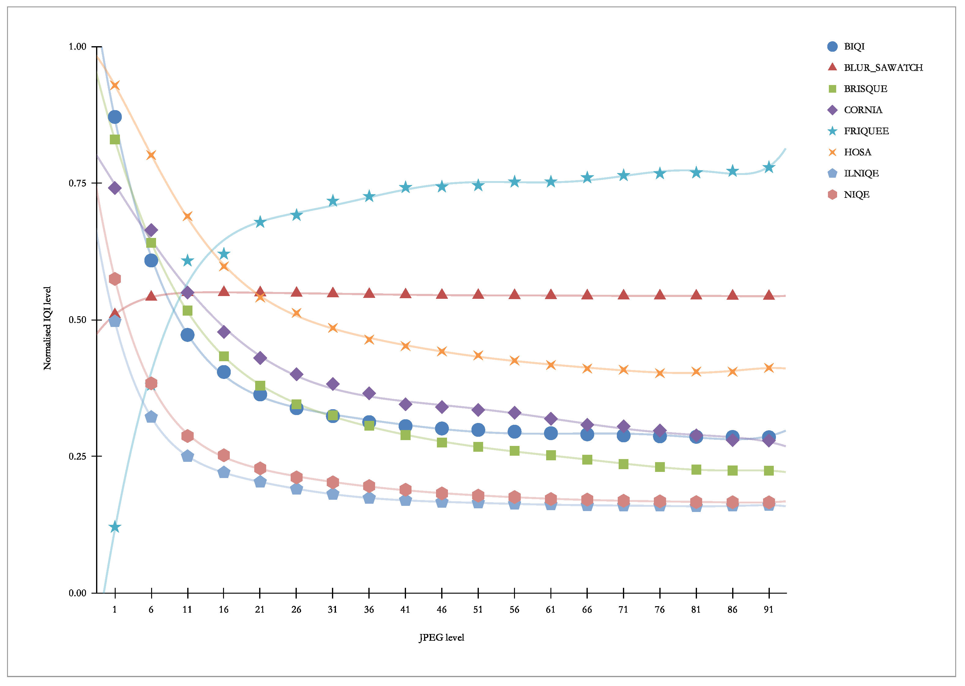
This subsection illustrates examples of the data that are obtained. Four distortions (HRCs) are selected for the imaging: defocus, Gaussian noise, motion blur, and JPEG. Two plots are plotted for each of the HRCs. One presents eight exemplary “Our” (made by AGH) visual indicators (selected indicators are: BLOCKINESS, BLOCKLOSS, BLUR, CONTRAST, EXPOSURE, INTERLACE, NOISE, and SA). The second one presents eight exemplary “Others” (made by other laboratories) visual indicators (indicators selected are: BIQI, BLUR_SAWATCH, CORNIA, FRIQUEE, HOSA, ILNIQE, and NIQE).
Figure 15 presents “our” indicators vs. Defocus. As we can see, this distortion causes the response of the BLUR indicator and, to a lesser extent, the SA indicator.
Figure 16 presents “other” indicators vs. Defocus. As we can see, this distortion causes the response of the FRIQUEE indicator and, to a lesser extent, the NIQE indicator.
Figure 17 presents “our” indicators vs. Gaussian Noise. As we can see, this distortion causes the response of the NOISE indicator and, to a lesser extent, the SA indicator.
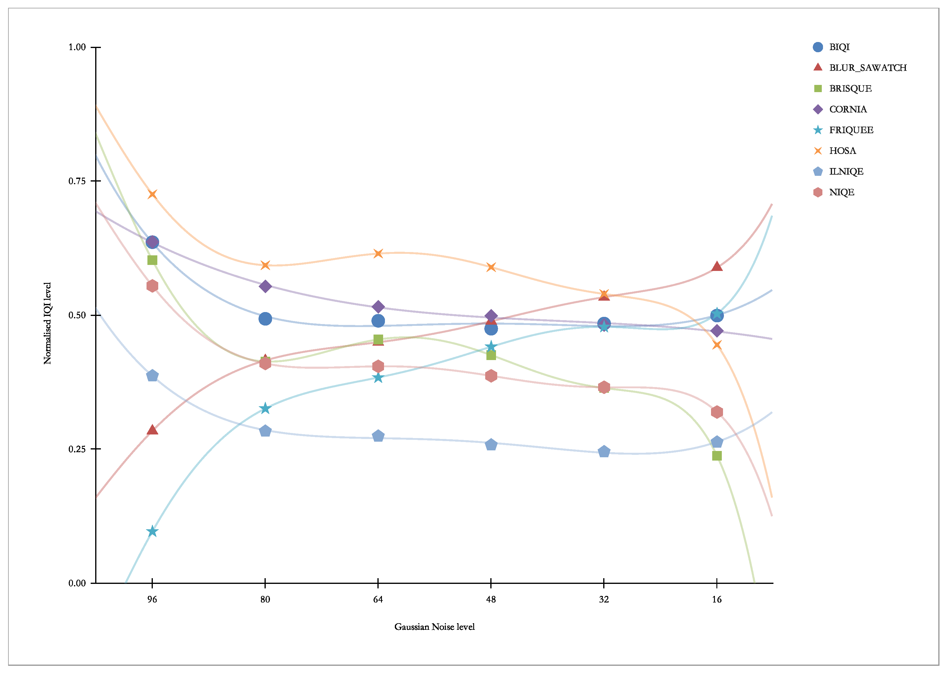
Figure 18 presents “other” indicators vs. Gaussian Noise. As we can see, this distortion causes the response of the FRIQUEE indicator and the NIQE indicator, and, to a lesser extent, also of the BRISQUE indicator.
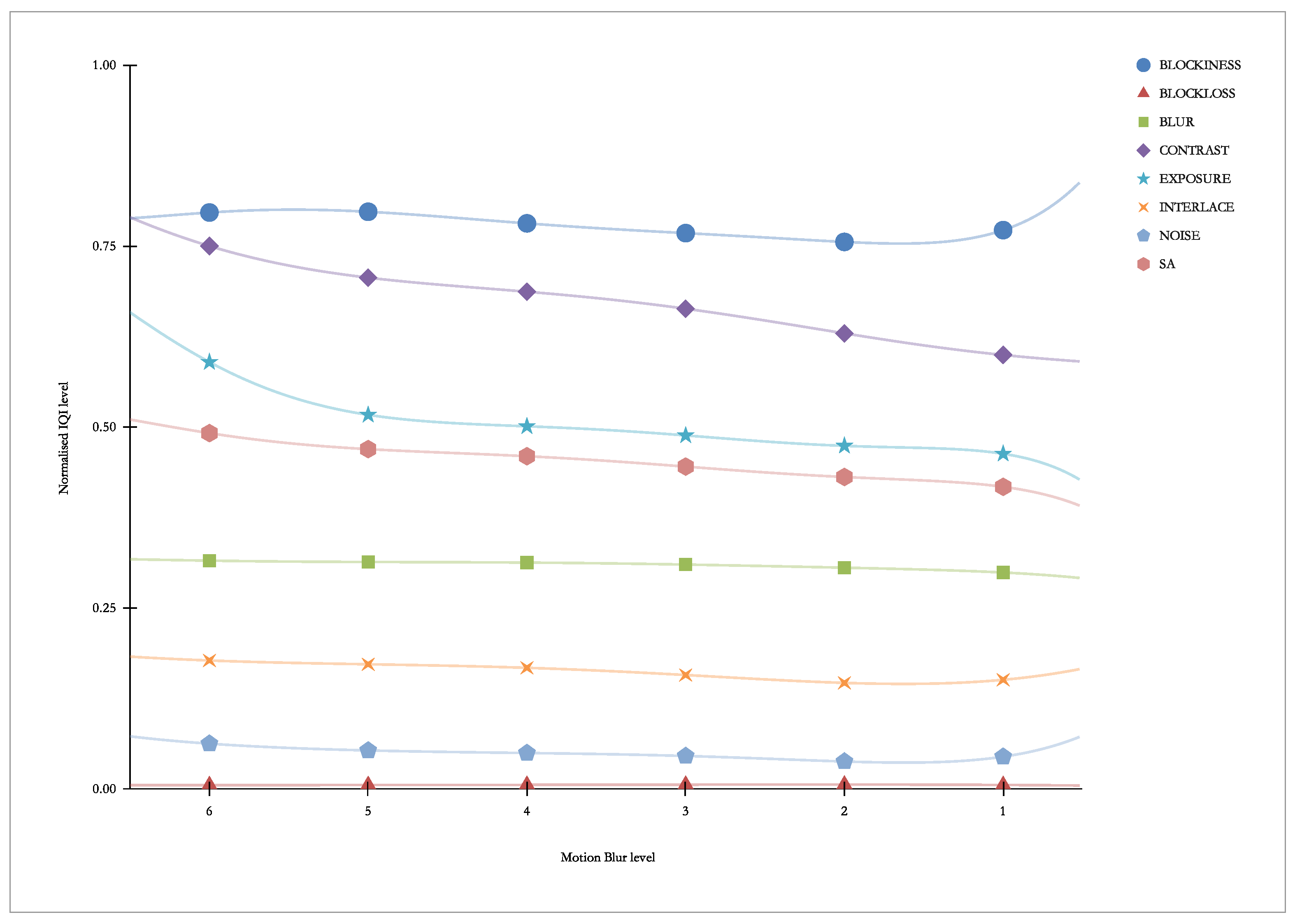
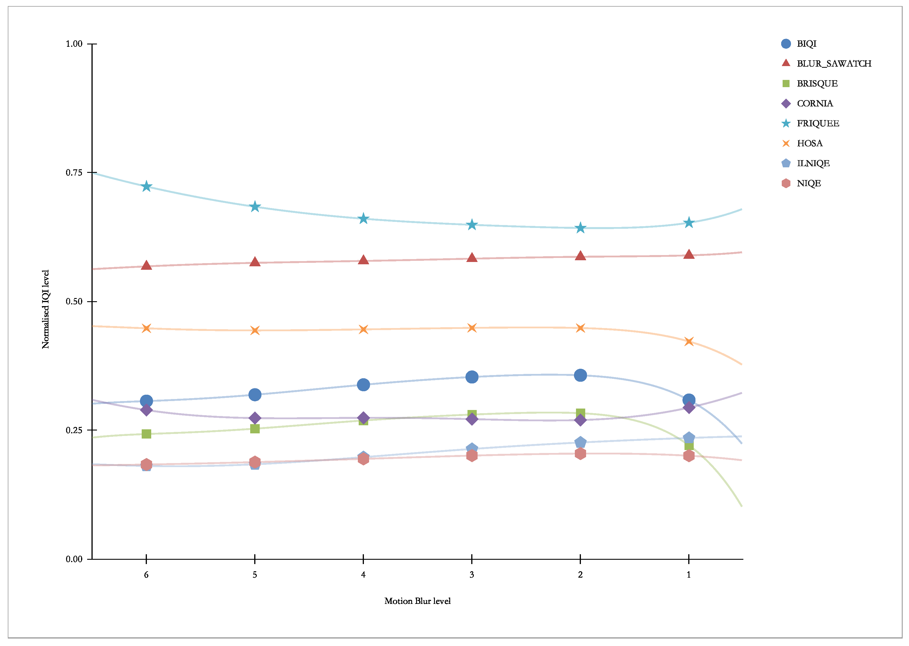
Figure 19 presents “our” indicators vs. Motion Blur. As we can see, this distortion practically does not elicit a greater response for any of the indicators.
Figure 20 presents “other” indicators vs. Motion Blur. As we can see, this distortion practically does not elicit a greater response for any of the indicators.
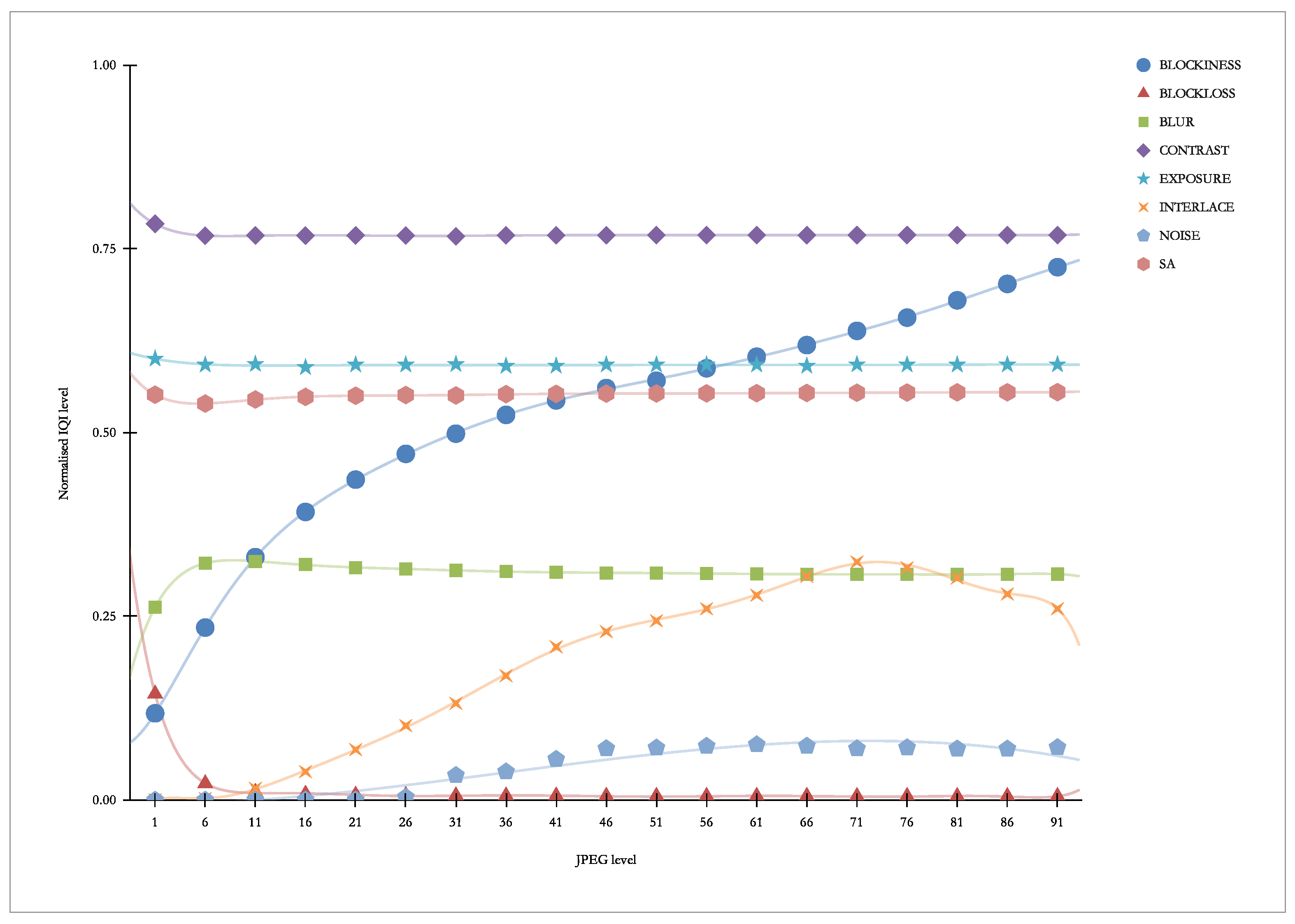
Figure 21 presents “our” indicators vs. JPEG. As we can see, this distortion primarily causes a strong response of the BLOCKINESS indicator (it is not surprising, as this indicator was created for this purpose).
Figure 22 presents “other” indicators vs. JPEG. As we can see, this distortion causes a strong response from virtually all indicators (especially for the lower range), except for BLUR_SAWATCH.
3. Results
This section presents the results of the development of a new objective video quality assessment model for face recognition tasks.
Possession of the two datasets (coming from the recognition experiment and the quality experiment) allows us to construct models predicting recognition results based on VQIs. The outcome is a new quality model. Importantly, such a model can be used even if there is no target to recognise. In addition, the information from the model and a recognition algorithm can vary.
We carry out modelling on two groups of VQIs. The first group are all available VQIs (both our own and those from third parties), which we mark as “All metrics”. The second group are exclusively our VQI, which we mark as “Only ours”.
We provide the results using standard values used in pattern recognition, information retrieval, and machine learning-based classification—Precision, Recall and F-measure. Precision (also called positive predictive value) is the fraction of relevant instances among the retrieved instances, while Recall (also known as sensitivity) is the fraction of the total number of relevant instances that were retrieved. Both Precision and Recall are therefore based on an understanding and measure of relevance. A measure that combines Precision and Recall is the harmonic mean of Precision and Recall, the traditional F-measure or balanced F-score [
41].
We test: Support-Vector Machine (SVM), Random Forest (RF), and Neural Networks (NN), searching the hyper-parameter space by grid search method. All methods provide very similar results. Finally, modelling using NN turns out to be the most effective. We use tensor flow to estimate NN parameters. First, we select the loss function and optimiser set to SparseCategoricalCrossentropy with the option from_logits=True and adam. Preliminary tests show that 20 epochs is enough, and the activation function relu shows the most promising results. The final tuning needs the number and structure of the layers. We consider up to three fully connected hidden layers with a number of neurons: layer0: [3, 6, 12, 24, 48], layer1: [0, 6, 12, 24], and layer2: [0, 3, 6], where 0 means that this layer is missing. Of course, 0 on layer1 means that layer2 also has the value 0. The final model has two hidden layers, with 48 and 24 neurons for the first and second layer.
We assume a classification into two classes (the face is recognised, the face is not recognised). We obtain the following (
Table 5) results.
Moreover, delving more into detail,
Table 6 shows the results we received for face recognition.
A more detailed analysis of the results obtained is also carried out. More specifically, two analyses are carried out: random visual inspection and numerical analysis of all data.
Regarding visual inspection, it is not easy to do because there are about 6600 images to be analysed. Therefore, the focus is on borderline cases—i.e., what the images look like, which, for a given distortion (only single HRCs are analysed):
They are not recognised well, even though the distortion is low.
They are still recognised well, even though the distortion is high.
For each case, some sample images are taken.
The conclusions are as follows:
There is probably a significant impact of SRC because there are images that begin to stop being recognised very quickly, despite the small HRC (incorrectly recognised images often come from the same repetitive SRC).
No similar effect is observed the other way around—extremely well-recognisable images with strong distortion rather seem a coincidence/luck (correctly recognised images usually come from different, non-unique SRCs).
By way of inspection, no random errors are found, such as damaged files, distorted images, etc.
The numerical analysis is to check the sensitivity of the model to individual distortions.
Figure 23 shows the share of erroneous predictions for a given HRC (the analysis is carried out for the case of the model using all VQIs, and the analysis for a subset of the VQIs shows practically very similar results).
As one can see, for the first four HRCs, the model shows quite similar error sensitivity—it is wrong in about a dozen or twenty percent of cases. The exception is JPEG HRC, for which the model is much less mistaken—only for 4% of cases. The explanation for this phenomenon could be that VQIs were created primarily to assess compression distortions. Hence, they are highly sensitive (thus discriminate) to the distortions introduced by the JPEG codec. Additional confirmation of this fact could also be the relatively low sensitivity to defocus distortion (14%), which is visually quite similar to compression blur.
4. Conclusions
We show in this study that the implementation of the new concept of an objective model to evaluate video quality for face recognition tasks is feasible. The achieved value of the model accuracy (F-measure parameter) is 0.87.
When all potential VQIs are used (VQIs by AGH and other research teams), the best modelling results are obtained. Nevertheless, it is worth noting that the restriction of AGH VQI does not lead to a significant decrease in prediction accuracy (F-measure of 0.83).
It is worth mentioning what causes the most typical problems encountered by the models during their work. Our observations suggest that the characteristics of the initial scene are an important component that misleads the models. VQI completely disregards this factor, which has a major impact on the recognition accuracy.
Of course, the limitations of the proposed method have to be mentioned. The method has been validated on a specific dataset, with specific image distortions and using a specific face recognition system. In addition, while the model is probably generalisable to other sets of faces, perhaps to other image distortions, and perhaps even to other face recognition systems, it is certainly not generalisable to other image recognition systems (e.g., object recognition systems or automatic number plate recognition systems)—which is evident from other (as yet unpublished) studies by the authors. For the same reason, it is also difficult to compare the obtained model with other methods. As mentioned in the Introduction, other published methods focus primarily on a completely different data modality and different recognition systems.


