Article

Time Series Segmentation Using Neural Networks with Cross-Domain Transfer Learning

1
Associação Fraunhofer Portugal Research, Rua Alfredo Allen 455/461, 4200-135 Porto, Portugal
2
Laboratório de Instrumentação, Engenharia Biomédica e Física da Radiação (LIBPhys-UNL), Departamento de Física, Faculdade de Ciências e Tecnologia (FCT), Universidade Nova de Lisboa, 2829-516 Caparica, Portugal
*
Author to whom correspondence should be addressed.
Electronics 2021, 10(15), 1805; https://doi.org/10.3390/electronics10151805
Submission received: 24 June 2021 / Revised: 21 July 2021 / Accepted: 22 July 2021 / Published: 28 July 2021
(This article belongs to the Special Issue Application of Neural Networks in Biosignal Process)

Abstract

:
Searching for characteristic patterns in time series is a topic addressed for decades by the research community. Conventional subsequence matching techniques usually rely on the definition of a target template pattern and a searching method for detecting similar patterns. However, the intrinsic variability of time series introduces changes in patterns, either morphologically and temporally, making such techniques not as accurate as desired. Intending to improve segmentation performances, in this paper, we proposed a Mask-based Neural Network (NN) which is capable of extracting desired patterns of interest from long time series, without using any predefined template. The proposed NN has been validated, alongside a subsequence matching algorithm, in two datasets: clinical (electrocardiogram) and human activity (inertial sensors). Moreover, the reduced dimension of the data in the latter dataset led to the application of transfer learning and data augmentation techniques to reach model convergence. The results have shown the proposed model achieved better segmentation performances than the baseline one, in both domains, reaching average Precision and Recall scores of 99.0% and 97.5% (clinical domain), along with 77.0% and 71.4% (human activity domain), introducing Neural Networks and Transfer Learning as promising alternatives for pattern searching in time series.

1. Introduction

1.1. Motivation

Over the last two decades, time series analysis became an attractive field to the research community (as seen by the rise in published studies), mostly due to the increasingly easier availability and collection of temporal data through several accessible devices (e.g., smartphones, wearables) [1]. Within the analysis of time series, the pattern recognition domain has attracted many researchers [2], since those patterns represent cyclical or seasonal oscillations that tend to mirror real-world phenomena whose detection cannot be carried out directly but only through specific acquisition devices. In the biomedical domain [3], the automatic detection of specific patterns in biosignals provides relevant indicators which help clinical specialists to better monitor their patients (even in ambulatory context) or support their diagnostic decisions.
Looking to achieve automatic segmentation of patterns within longer time series, several techniques have been proposed. As each use-case returns morphologically distinct patterns, the methods should be well generalized to cover any data domain and scenario. Conventional techniques usually consist of a defined reference template, characterizing the pattern desired to match, and a distance metric (e.g., Euclidean Distance—ED, Dynamic Time Warping—DTW, Time Alignment Measurement—TAM [4], among others) measuring the similarity of that template relative to the portion of a signal evaluated [5]. An illustration of such an approach is displayed in Figure 1, where a template window is slid along with a longer time series at the same time a distance metric is computed.
Even though the aforementioned strategy might achieve some degree of generalization, real-world time series are variable (in a way, the morphology and duration of patterns might have an intrinsic variability) and noisy [6,7]. Thus, a search reliant on a single template or metric (however flexible it may be) is not a robust approach, since it can lead to the loss of important patterns [8]. Some examples of types of distortion in temporal patterns are displayed in Figure 2.
In order to increase the flexibility of pattern segmentation in time series, rendering the task less sensitive to the latter’s variable components, as well as less domain-oriented and conditioned to user parameter choices, in this paper, we propose a Deep Learning (DL) architecture that performs a point-by-point mask-based segmentation of time series. It associates each point with a confidence level of belonging to the pattern class (higher granularity than conventional template-based methods). Such mask-based neural network models are capable of rejecting noise and handling variability by themselves [9], i.e., automatically, once fed with an appropriate training set. The proposal was tested with both univariate and multivariate signals. Regarding the multivariate setting, the lack of data motivated the implementation of a transfer learning approach and data augmentation, as well as an adaptation of the univariate architecture in order to handle multivariate time series.

1.2. Conceptual Background

In the Machine Learning (ML) field, there are two dominant categories of models (according to their purpose): discriminative and generative. The difference between both is what each model actually learns. While discriminative models aim to learn the decision boundary between some desired classes within a dataset (in order of distinguishing them), generative techniques focus on modeling the actual manifold distribution of such classes into a previously known distribution, thus gaining the ability to generate new artificial instances [10]. Since our goal rests on the segmentation of desired patterns in longer time series, generative models are out of the scope of this paper.
Discriminative models [11], thus, learn a function which allows the discrimination between classes/labels. It is traditionally used in pattern recognition tasks [11], and some of the most popular neural network discriminative architectures include Convolutional Neural Networks (CNN) [12], Recurrent Neural Networks (RNN) [13] and its Long/short term memory (LSTM) [14] implementation, among others.
There are many types of Deep Neural Network (DNN) architectures, each one incorporating its own unique combination of operations within hidden layers. We will focus on the definition of CNNs, which are the basis of our proposal.
Convolutional Neural Network (CNN) [12]:
A CNN is a feed-forward neural network, mostly associated with classification and regression tasks. Typically, in the first layers, several hidden layers compute consecutive convolutions to the input data, for feature extraction. Each convolutional layer is followed by a pooling one which shortens the input length. After that, the convolutional product is flattened into a set of one/few fully-connected layers to perform a decision-making task, allocating the input to its corresponding class (Figure 3).
An interesting variant of this CNN is the Convolution/Deconvolution Neural Network (see Figure 4).
It holds the same theoretical foundation as a simple CNN but has a different purpose since the input and output have the same length. Here, through the same set of operations, the input is encoded (first half of layers) to a latent dimension and decoded (second half of layers) until reaching the original input size. The only difference is that pooling layers compress the input in the first half, while unpooling ones are expanding it in the second half. Yet, depending on the loss function applied, the problem carried out may change. In autoencoders, the output is forced to be as similar as possible to the input, while, if a point-by-point classification (segmentation) task is followed, the output comprises a set of masks, where each time point is assigned to its corresponding class label, with a respective confidence level.

1.3. Related Work

When dealing with similarity among two sequences, the simplest measure consists of computing the ED (or any L p norm) between both series [17]. The higher the distance, the most dissimilar those sequences are. The main problem of such simple metrics is the lack of flexibility to find time or amplitude distorted patterns [18], and also to compute the similarity between unequal-sized subsequences. Trying to overcome these drawbacks, DTW has been proposed [19], being able to align temporally misaligned but morphologically similar sequences. This flexibility allows conventional techniques (that define pattern templates and search for matches along with time series) [20] to perform better in real-world problems. With respect to the Human Activity field, Nguyen-Dinh et al. [21] proposed two template-matching methods—using LCSS (Longest Common Subsequence Similarity)—applied on accelerometer data for online gesture recognition and reported accuracy scores 12% greater than existing template-matching techniques. Moreover, J. Barth et al. [22] implemented a template-based subsequence DTW technique to execute multi-cycle segmentation in gyroscope data collected from daily human activities, having achieved a step recognition rate of 97.7% (ten-meter walk) and 86.7% (daily life activities).
Despite being less sensitive to patterns’ intrinsic variability (shifting, scaling), DTW is sensitive to noise and computationally expensive, leading to an increased running time for many pattern-searching algorithms [23]. These issues discourage applying template-based segmentation techniques, supported by their dependence on predefined parameters and a single, rigid template.
Feature engineering-based techniques are also a common strategy for extracting relevant characteristics from time series. There are currently many tools following this type of analysis [24]. However, to solve segmentation tasks, those features must be combined with a searching method [18], which is not as common as their application in classification tasks (e.g., human activity recognition) [25].
More recently, DL models have started to be applied in time series analysis (concretely concerning classification and anomaly detection tasks) [26,27,28,29,30] after having achieved a notable success in the computer vision field [31]. DNN models offer many advantages when compared to classical approaches, since they do not require an elaborate data pre-processing pipeline, they are capable of efficiently extract relevant feature maps (unlike hand-crafted methods, which require expert domain knowledge and can be computationally more expensive to extract [32,33]), and better handle abundant amounts of data. Concerning cycle segmentation tasks, Perslev et al. [34] implemented a fully convolutional neural network with U-shape architecture, initially proposed for image segmentation tasks, working on electroencephalogram (EEG) sleep stages detection, through a mask-based segmentation model. It has been shown to outperform other neural network architectures, with averaged global F1-scores of 75.6% over seven different datasets. Another U-shape DNN has been proposed in [35], by Moskalenko et al., presenting a segmentation model for discriminating all the different complexes within an ECG cardiac cycle: P, QRS and T oscillations. It has reported F1-scores of, at least, 97.8%, 99.5%, 99.9% at detecting P, T, and QRS waves onsets and offsets, respectively. The same task has been introduced in [16], by Sereda et al., carried out by a sequential Convolutional/Deconvolutional NN model implementation, presenting averaged sensitivity and precision scores of 97.5% and 91.9%, corresponding, regarding ECG waves’ onset and offset detection.

1.4. Structure Outline

The rest of this paper is organized as follows: Section 2 holds the description, implementation procedure, and hyperparameter definition of both conventional and DL-based techniques, besides an introduction of two datasets considered for validation purposes. The Section 3 presents an overall depiction of both models’ performance concerning each one of the datasets, and the respective comparative discussion of the obtained visual and quantitative segmentation results. Finally, Section 4 ends up summarizing the experiments discussed throughout the paper, the major achievements, and future guidelines for research follow-up.

2. Methodology

In this paper, the proposed framework aims to study the automatic segmentation of patterns within time series based on DL. Additionally, a conventional approach has been implemented as a baseline for comparison with the proposed DL-based approach. Experiments were performed concerning both univariate and multivariate pattern analysis, using ECG and inertial sensor-based Human Activity signals, respectively.

2.1. Baseline Model

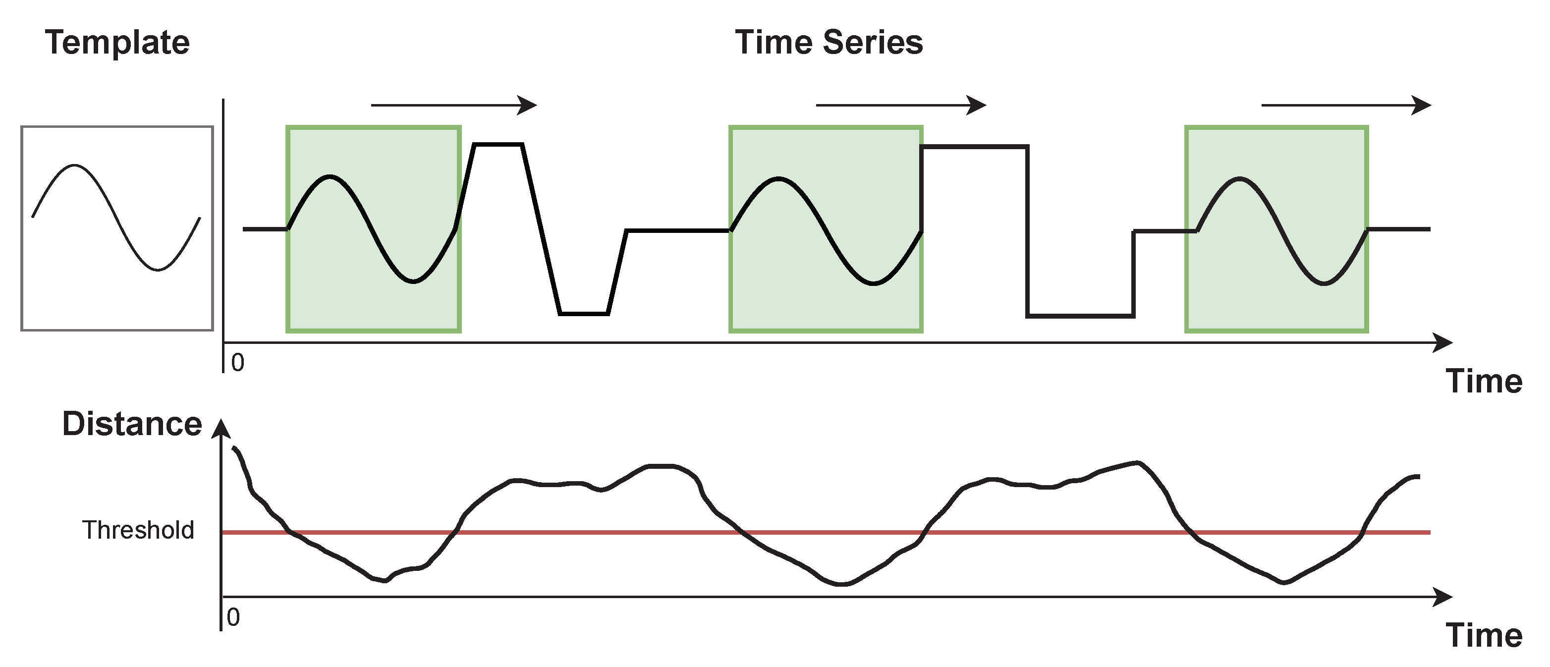
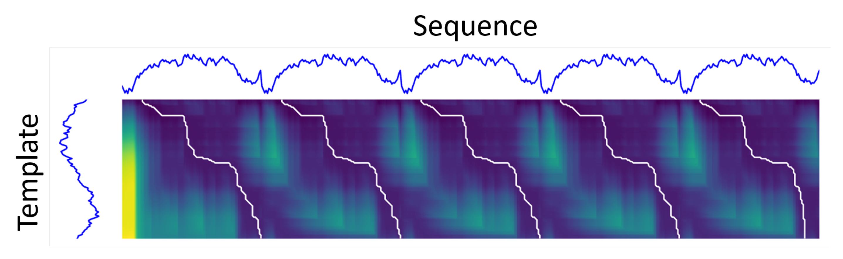
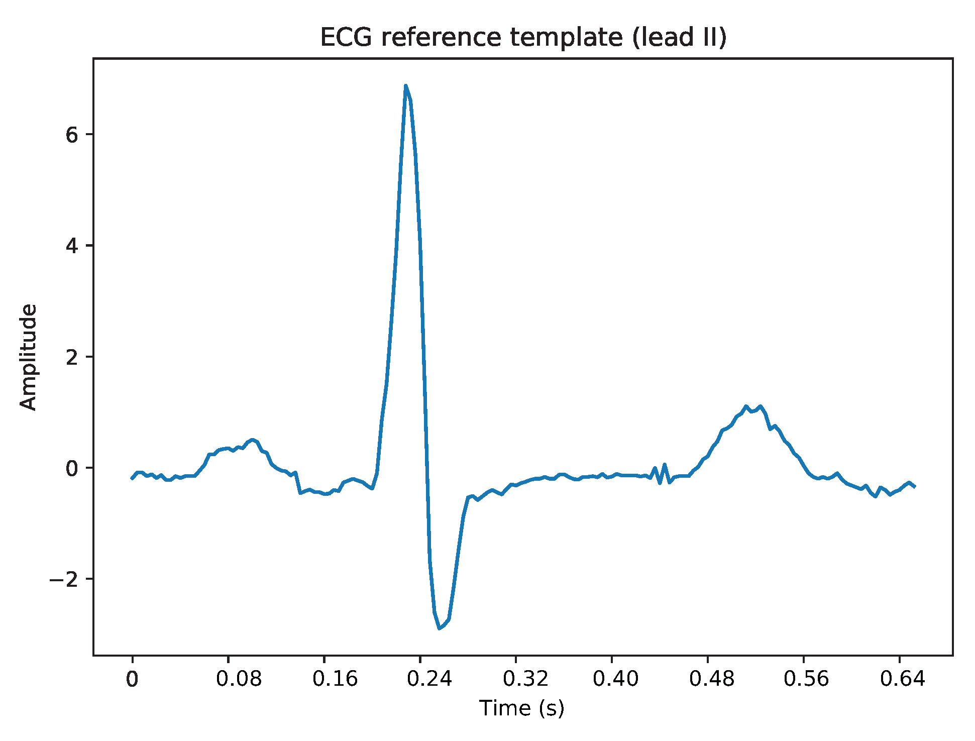
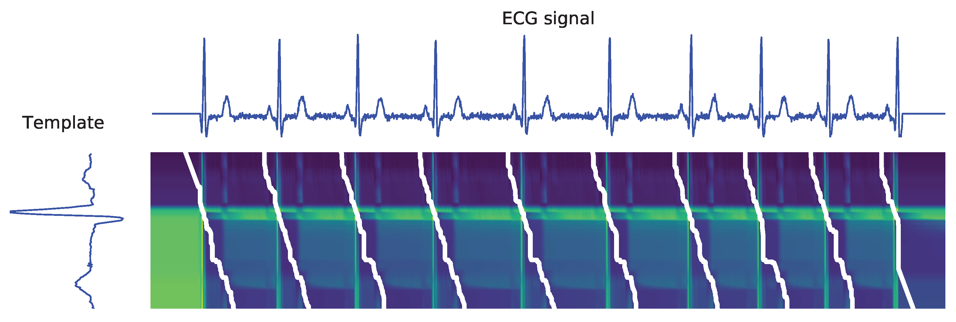
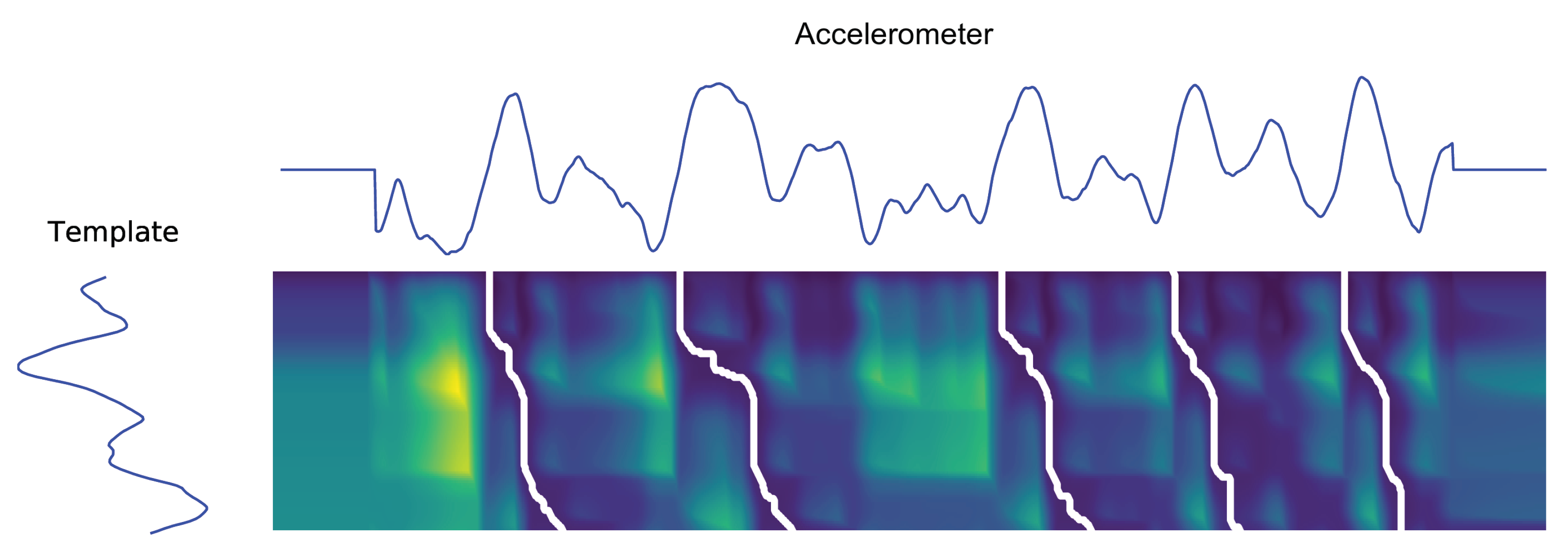
Subsequence Dynamic Time Warping (sDTW)

The sDTW algorithm is a template-based method for subsequence segmentation on time series, whose implementation is publicly available in the tslearn Python library [36]. While in several classical DTW techniques (e.g., vanilla DTW [37], SSDTW [38], W-DTW [39], CDTW [40]), the algorithms look to align both sequences in one single path, here a subsequence searching technique is applied to find multiple paths of a given reference pattern. Moreover, the main reason leading to the choice of sDTW as our baseline was that this method combines both pattern similarity and subsequence searching properties in one single approach. Additionally, its implementation is publicly available, which made reproducing the results easier.
Getting into detail on sDTW, this sub-warping technique uses a reference template (corresponding to the pattern of interest) which is compared with a longer sequence (containing multiple repetitions of that pattern), through the computation of a cost matrix measuring a metric distance, point-by-point. The process is, then, based in the cost matrix analysis, which searches for the alignment warping paths (between the evaluated and desired sequences) achieving an optimal overall distance/similarity relative to the desired pattern. The algorithm defines the squared difference score as the metric that generates the cost matrix (relating the point-to-point local alignment cost) and its subsequent accumulated version (reproducing the total alignment cost between [1, 1] and [n, m] cells). The user must still set two additional parameters tuning the function that finds the candidate paths: The minimum peak height, H, and minimum inter-peak distance, D. The function receives the symmetrical of the cost matrix’s last row, indicating the similarity relative to the template’s offset point, and finds its local maximum points (minimum in the original row), which represent the most similar points (with lower distance). The selected offsets must be separated, at least, by D points (assuming non-negative values) and assigned with a distance higher than H (values restricted within the [ , 0 ] interval). Following this reasoning, lower H values lead to more selected candidate offset points, and consequently, more alignment paths. The same happens for lower D values, and vice versa. Figure 5 helps to illustrate the overall technique.
As the sDTW algorithm requires the selection of an amplitude threshold (H parameter), the inherent variability of the raw signals could eventually raise the cost matrix values in regions where patterns are present, and miss their matching. Aiming at overcoming that limitation, either the longer sequence and template signals were normalized by the maximum of its module so that the cost matrix values became constrained. Moreover, two divergent paths could be associated with the same onset point. In such cases, an additional rejection criterion has been applied to exclude the path whose length is farther from the template’s.

2.2. Univariate Analysis

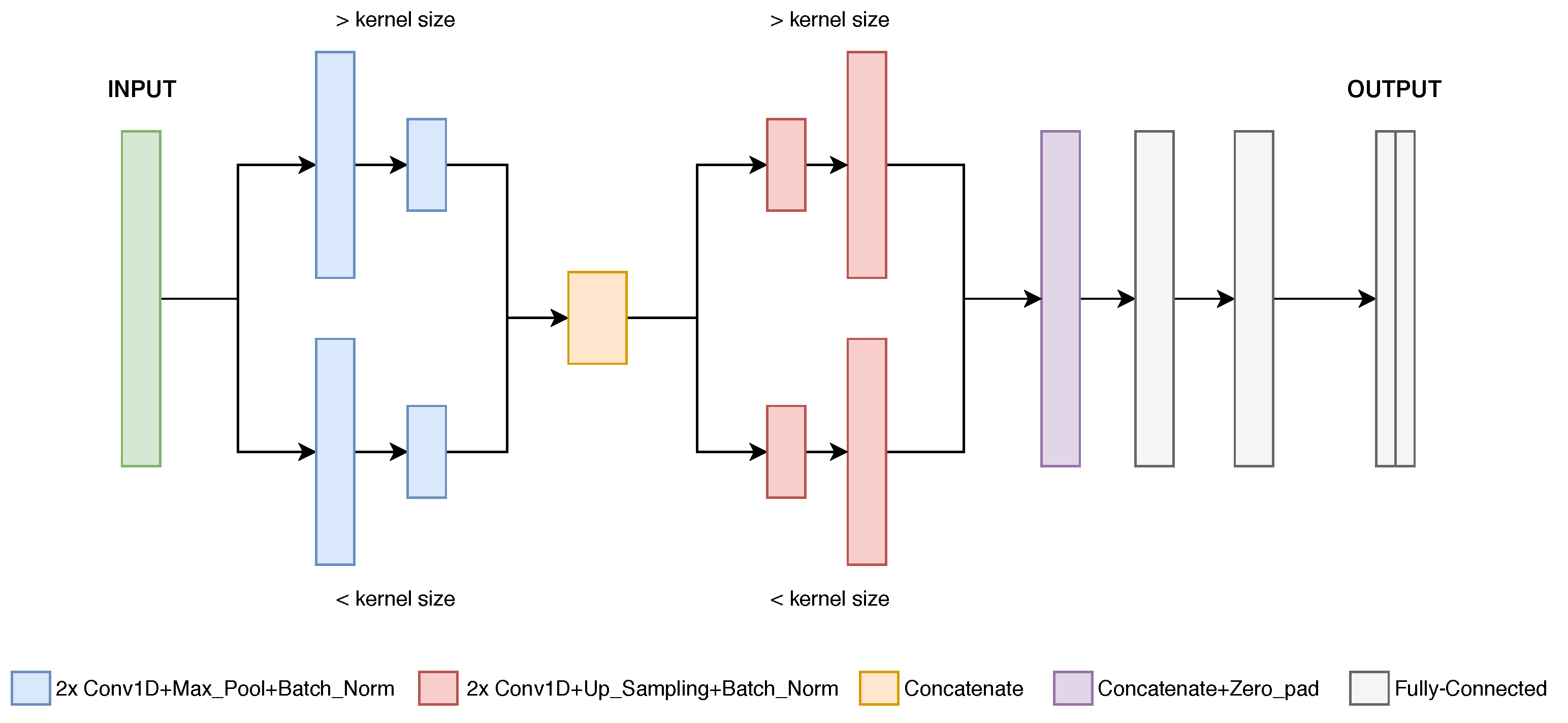
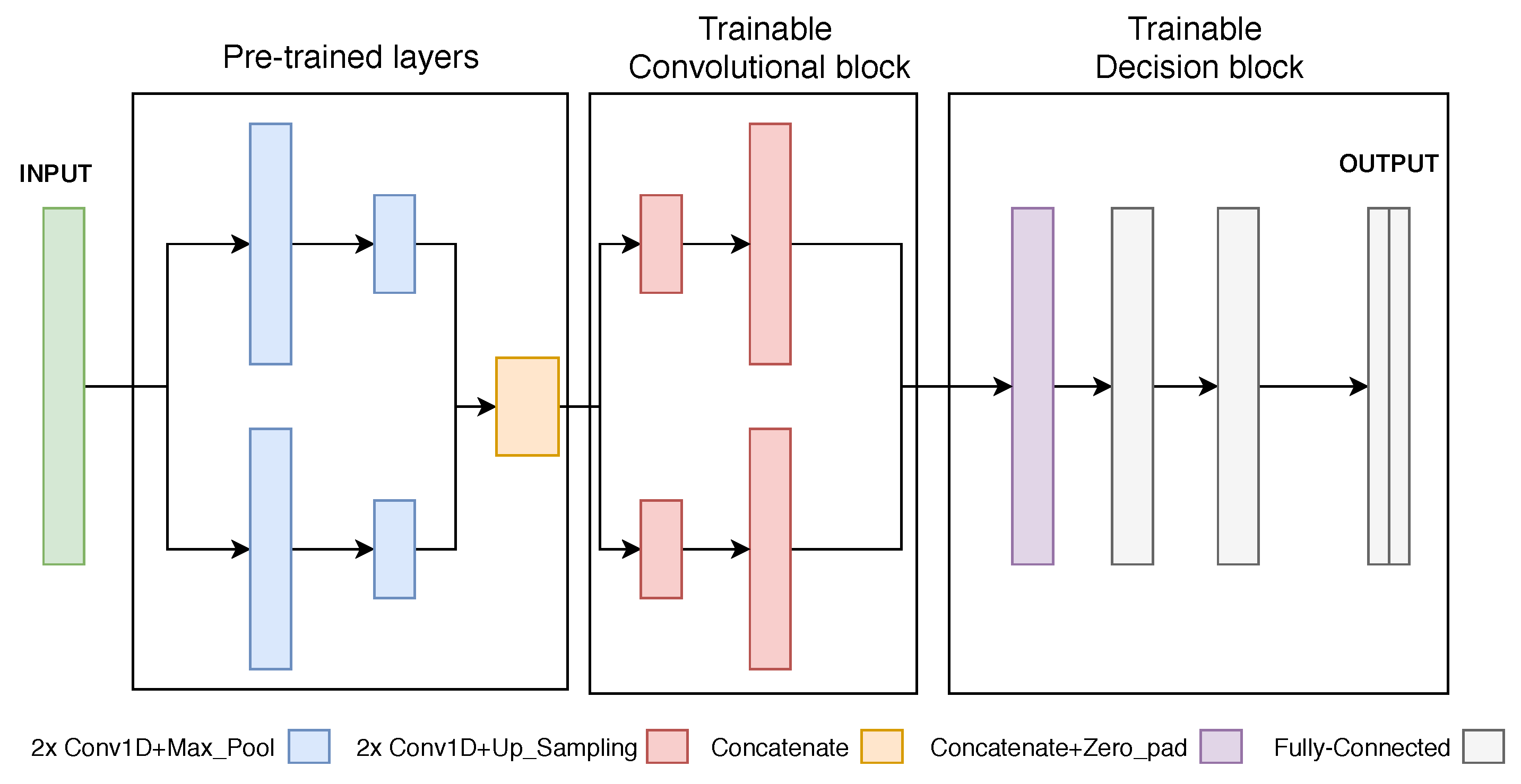
2.2.1. Proposed Model

The proposed DL-based architecture has been named “Hourglass”, since it comprises two consecutive pairs of parallel paths with convolutional layers each, resulting in a shape similar to an hourglass (see Figure 6). The difference between both paths is the convolutional kernel size, larger in one path and shorter in the other. The motivation is to achieve feature extraction with distinct temporal resolutions (employing simultaneous global and local feature extraction), followed by a concatenation, helping the model decision task. In the final layers, the convolutional product passes through a set of three fully-connected layers, to perform a point-by-point classification. The output is composed of N binary channels/masks (being N the number of classes), each one containing each point confidence level relative to that class.
This approach is based on convolutional compression (pooling) and expansion (unpooling) and is frequently introduced in image segmentation tasks [41], so an analogous 1D-oriented neural network has been implemented.
Convolutional layers are linked with a Pooling/Unpooling layer, to compress/expand the input data, and a Batch Normalization layer, to enable a faster model training convergence (avoiding overfitting) [42]. One path works with a larger convolutional kernel (30 points), whereas the other is reduced (8 points). The number of convolutional filters varies between 32 and 8 in both paths.
The proposed CNN was compared with other architectures (proposed in [16,35]), in a similar problem and, regarding preliminary experiments, it has shown competitive performances, which supports the Hourglass CNN choice. Since the architecture’s choice is out of the main scope of this work, we refer to a summary of some performance metrics over the three considered networks in Table A1, in the Appendix A.

2.2.2. LUDB Dataset

The Lobachevsky University Electrocardiography Database (LUDB) [43] is an open-access dataset, containing ECG records from 200 different individuals. Each recording represents a 10-s ECG signal, acquired with 12 leads and a sampling rate of 500 Hz, whose cardiac cycles have their waves (P, QRS, and T) individually annotated by specialists. Figure 7 illustrates how cardiac cycles were annotated in separate segments.
The dataset contains one ECG signal per individual, so the splitting process became straightforward at ensuring each subject’s cycles are not included in different sets. Therefore, three subsets of signals were considered: training, validation, and a testing set (Table 1).

2.2.3. Pre-Processing

Firstly, the ECG lead II has been defined as the channel of analysis for this univariate pattern segmentation task. In fact, this is the most widely used lead to access the cardiac rhythm in ECG analysis [44], showing the three main ECG waves (P, QRS, and T) well amplified and discriminated (the lead’s dipole follows the myocardium’s depolarization direction).
Secondly, the LUDB dataset exhibits a particular characteristic, where the first and last cardiac cycles are not annotated. To prevent an increase in false positives, signals were cropped on both extremes (as performed in [35]), so that the first and last heartbeats were removed. Moreover, three classical pre-processing steps (see Figure 8) were executed:
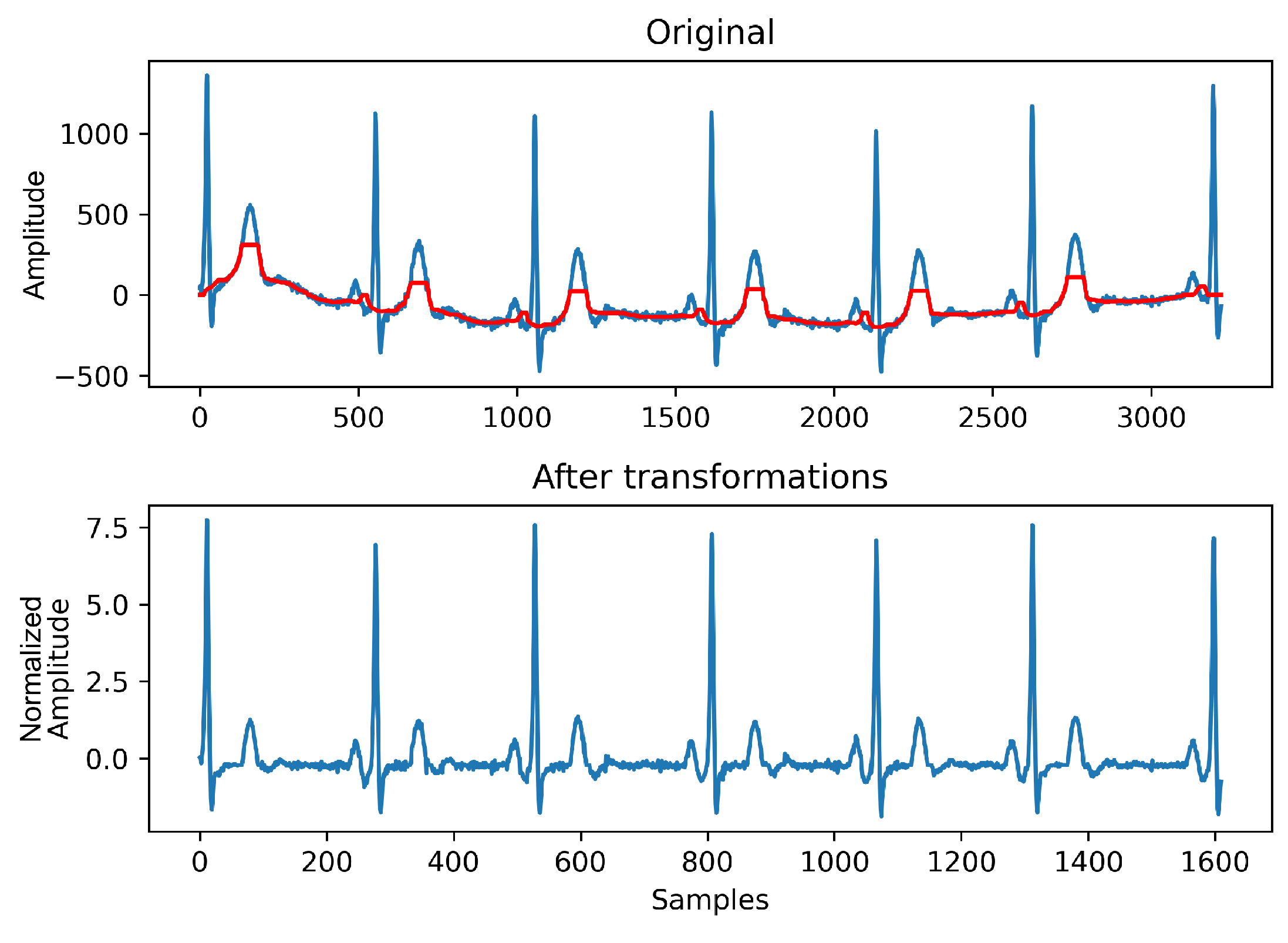
  • Baseline wander removal: The application of two consecutive median filters (with 0.2 and 0.6-s sized kernels, in this order) [45], rectified ECG waves and baseline drift was partially removed;
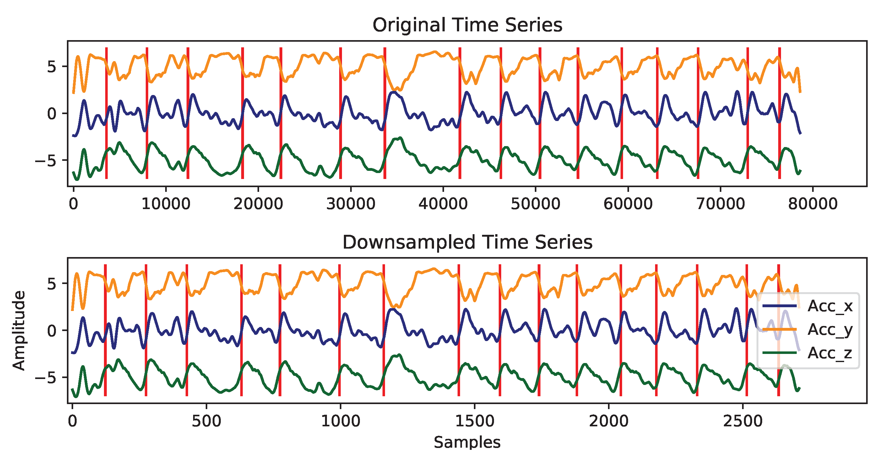
  • Downsampling: signals were downsampled by a factor of two, to reduce the computational cost of the associated segmentation algorithms. The sampling rate was reduced to 250 Hz;
  • Standardization: The final step consisted of constraining the amplitude range of signals as follows:
    X n o r m = X r a w μ σ ,
    where μ and σ represent the signal mean and standard deviation, correspondingly.
High-frequency noise has not been removed, in a way to test the model’s robustness to reject noise components. Furthermore, shorter signals were padded with zeros on both sides to set a fixed input size for the NN.
Finally, regarding the annotation of P, QRS, and T segments, they were merged into a complete cardiac cycle, accounting for their temporal order within the cycle (it starts with a P wave and finishes with a T wave), in order to enable the execution of a Beat vs. Background segmentation which seemed a more suitable task for flexible matching evaluation.

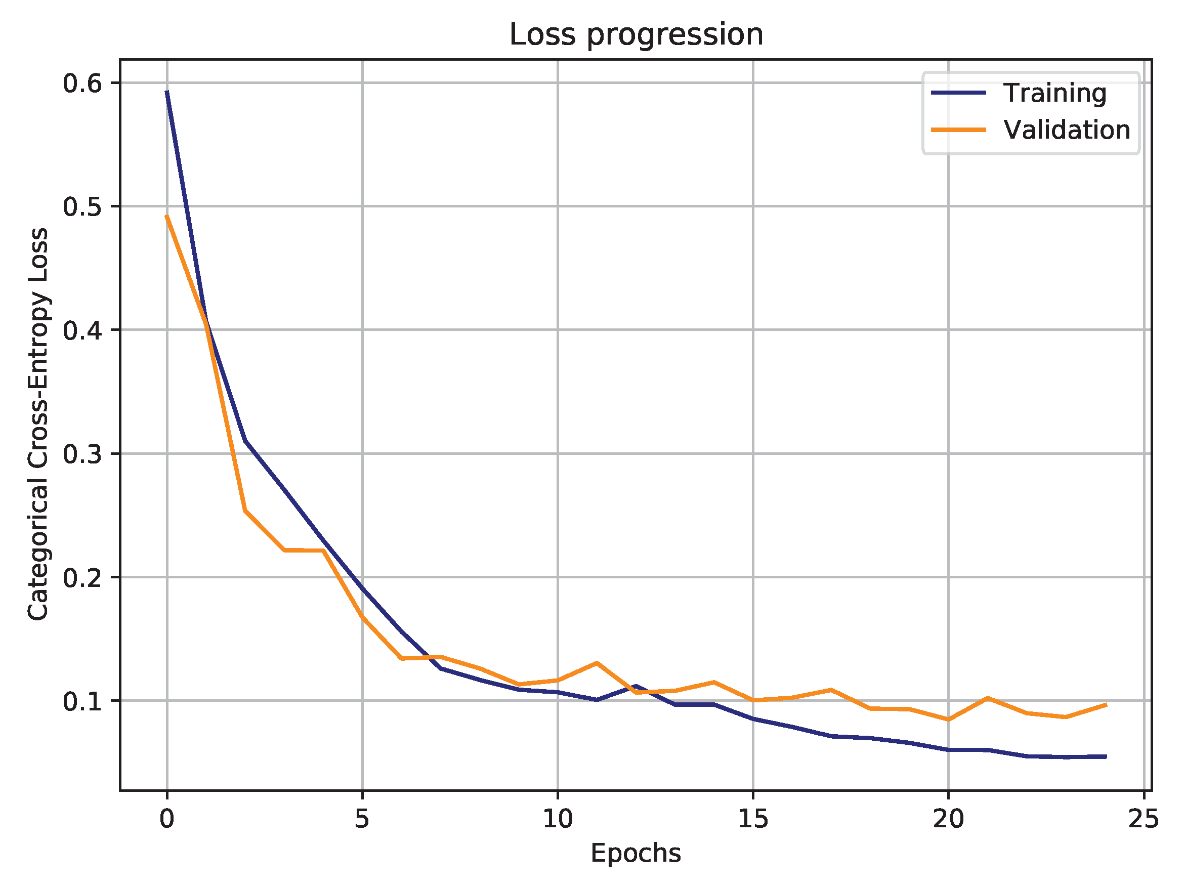
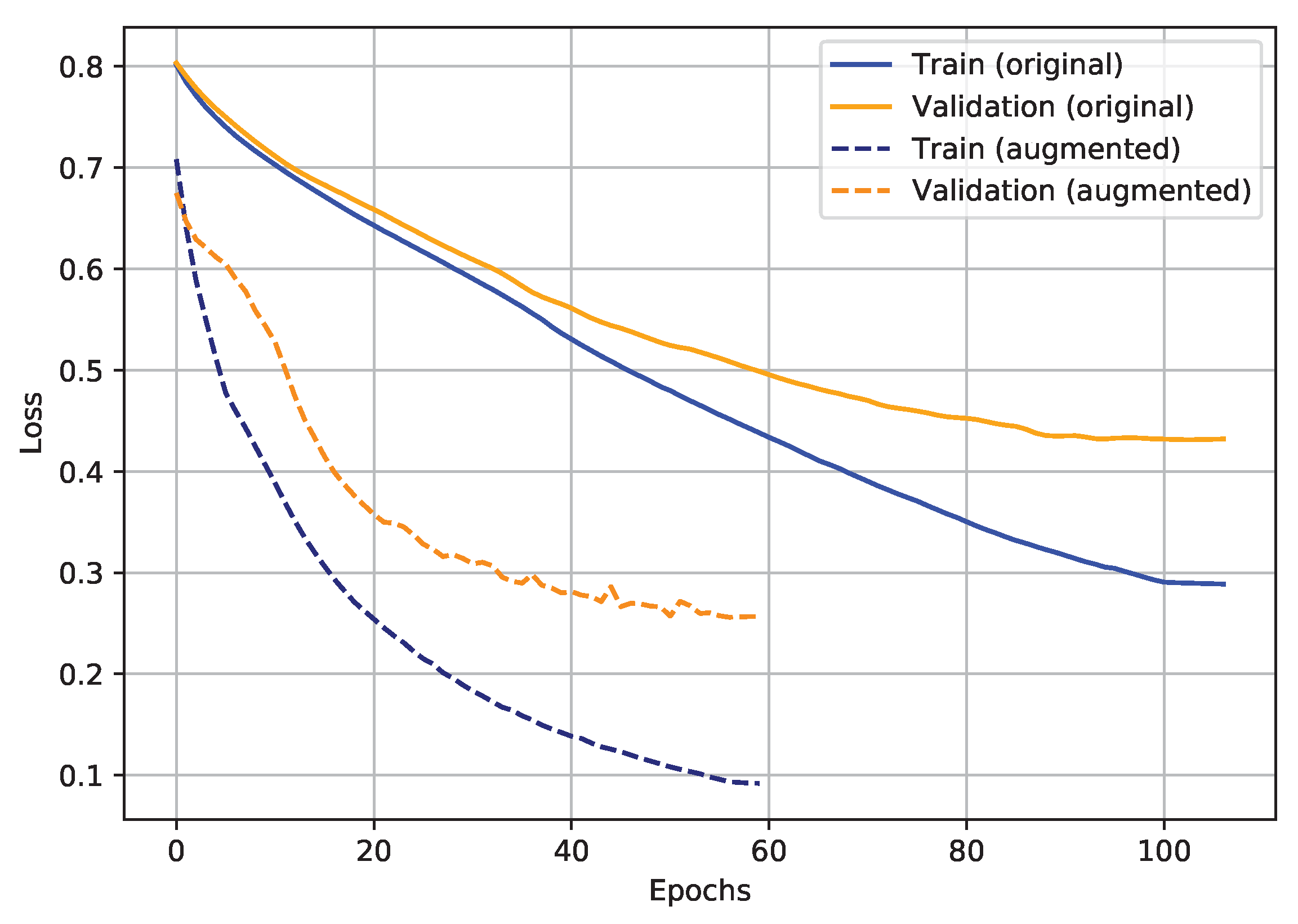
2.2.4. Training Stage

At the training stage, the proposed NN has learned from training data, while validation samples have guided the learning step, tuning the model hyperparameters, avoiding overfitting, and maximizing the pattern recognition capabilities within the provided time series (ECG signals). The hyperparameter settings applied are shown in Table 2.
The Cross-entropy error function has been used as the network’s loss due to its differentiability and common applicability in classification tasks. The number of selected epochs is explained in Section 3.1. The hyperbolic tangent (tanH) function has been defined as the main activation of the network layers since it can handle both positive and negative values, which is precisely the range of values of the input signals. Relative to the batch size, it is arbitrary but not too small to enable (along with the aforementioned Batch Normalization layers) the use of a higher learning rate.

2.2.5. Baseline Model Parameters

For establishing a comparison with the proposed DL model, the sDTW technique has been introduced. Although it does not involve a training step, it requires the definition of a reference template and other two additional parameters (tuning the function that finds the offset points). The two parameters were set as indicated in Table 3.

2.3. Multivariate Analysis

The following experiment introduces an adaptation of the previously described Hourglass CNN in order to handle multi-channel time series, as well as the application of Transfer Learning to improve training.

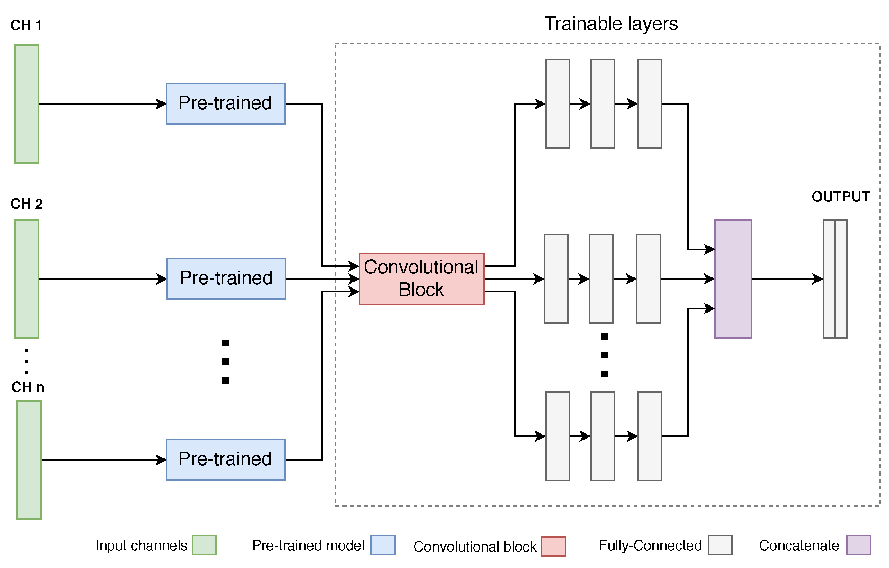
2.3.1. Proposed Model

Some datasets do not have a sufficient data volume or diversity for training DNNs efficiently, especially multivariate datasets. Several techniques can be applied to overcome such issues, one of which concerns a Transfer Learning approach [46]. The idea behind it is based on training some network layers with data from other domains (with more available data), whose general knowledge (in the form of weights) will be extracted and transferred to a similar architecture to train the target dataset.
During the new training steps, the pre-trained layers can have their weights frozen (no update), reducing the number of trainable parameters and possibly preventing the network from overfitting. After some learning steps, those weights can be unfrozen and carefully optimized towards the desired target domain (fine-tuning). In this case, the Hourglass CNN was used as a base model for the pre-trained model (Figure 9). The first convolutional pair of branches compose the pre-trained portion of the network since the first layers are assumed to be responsible for extracting the most general features from the data [46], common across different domains. A subsequent decision-making set of fully-connected layers was included, returning, in the end, N equal-sized output masks.
In order to provide a multivariate signal analysis, a new architecture has been implemented, adapted from the univariate version (Figure 10).
As the pre-trained network was trained with univariate data, each individual channel is passed through a pre-trained block and then through a shared trainable convolutional block (also present in the univariate version). Finally, each channel diverges into its own set of decision-making layers, whose outcome is concatenated and mapped to the final output mask.
According to the type of problem at hand, one can add/remove as many channels as needed. Nonetheless, one must note that adding more channels will increase the variance of the data and the complexity of the whole network.

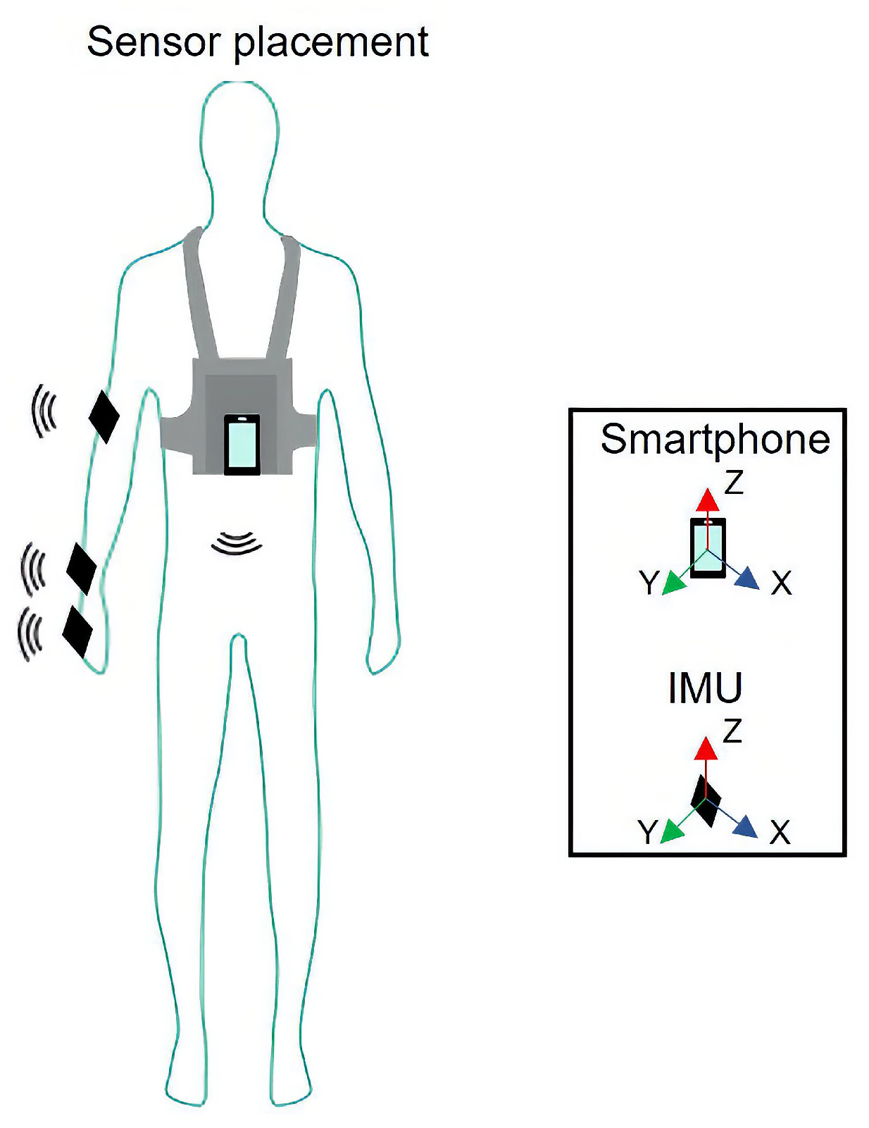
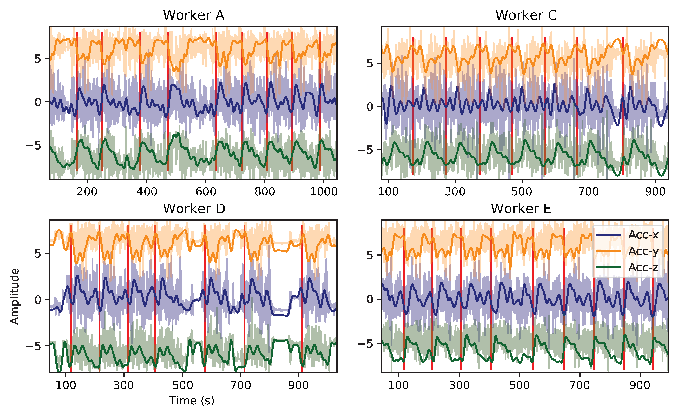
2.3.2. Human Activity Dataset

This dataset contains human activity data extracted from several subjects working in an industrial environment [47]. In large manufacturing sites, predetermined motions are defined for each task. The ideal method to perform such tasks aims to achieve the best performance: increase productivity ratios and reduce ergonomic risk. The operators execute, continually, during their work shift, iterations of the same task using repetitive movements. A work cycle is an individual iteration of a given task. Several types of data were collected, including electromyography, video, and inertial measurement unit (IMU) data, while each worker executed distinct activities, associated with different workstations of a given industrial assembly line. In each acquisition, four IMUs were positioned in different anatomical segments: hand, wrist, elbow (of the dominant arm), and chest (see Figure 11). Each IMU contains three sensors: an accelerometer, a gyroscope, and a magnetometer. Each sensor collected data at 100 Hz , in three orthogonal directions, conventionally called X, Y, and Z. Summing up, each individual data acquisition has 4 × 3 × 3 = 36 channels.
This study did not comprise any data collection stage. All the concerns about the collection stage proceedings and participants informed consent should be consulted in [47].
Regarding the workstation tasks, two key activities were considered: Liftgate, Fender. Signals were collected from ten different subjects/workers. Yet, due to some signal quality issues (noticed during the acquisition and after observing the raw signals), only five subjects (from the total ten) and specific sensor positions (which captured amplitude-relevant patterns during the task execution) were selected for the analysis:
  • Workers: A, B, C, D, E;
  • Workstations: Fender, Liftgate;
  • Sensors: Elbow, Wrist, Chest.
Signals were additionally cropped into smaller temporal windows to increase the number of training samples. So, each worker can have more than one associated sample. Table 4 shows the total number of samples per activity and worker, available to perform both training and validation steps.
Finally, three out of nine available channels of each IMU were considered (corresponding to the three axes of the accelerometer sensor), to limit the computational cost of this segmentation task and reduce overfitting of the network (adding more channels increases the network complexity).
Regarding evaluation, a leave-one-worker-out evaluation strategy was chosen, since it is an unbiased technique and not too computational expensive given the small amount of data [48]. It consists of assigning a single worker, at a time, to the validation set (instead of a particular sample) and the remaining workers on the training set.

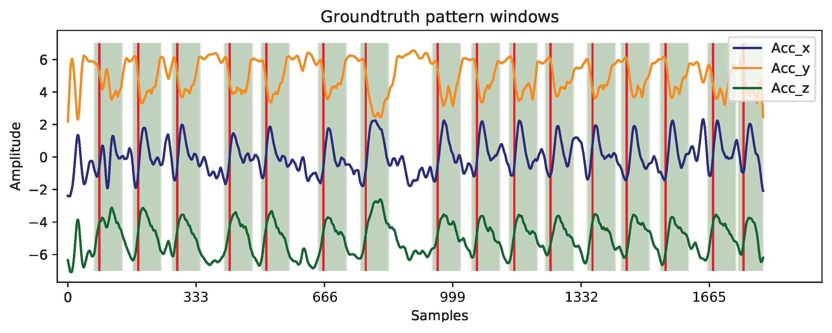
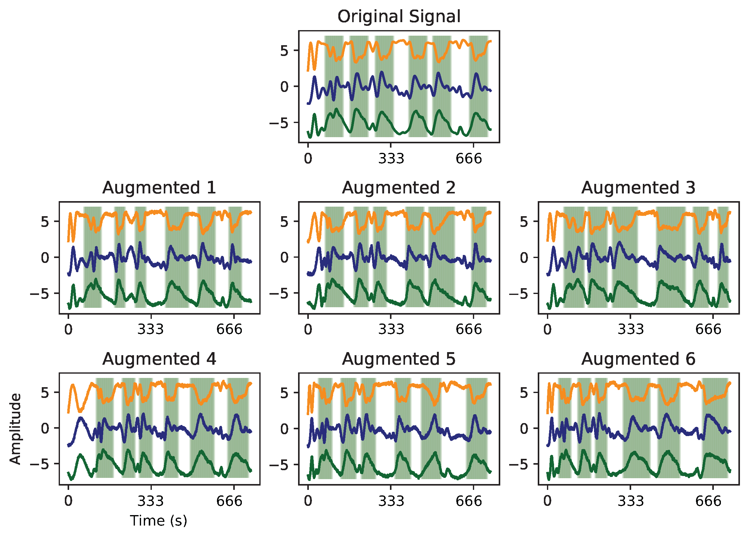
2.3.3. Pre-Processing

All the transformations applied to the raw input signals and their target classification masks before they are fed to the segmentation model, will be described in this subsection. The following figures display some inertial sensor signals where a different amplitude offset factor has been applied to each channel, simplifying their visualization.
Filtering
The application of a Butterworth Lowpass filter (3rd order, with 0.05 Hz cutoff frequency) successfully attenuated non-desired high-frequency content, and enhanced human activity signal components, as depicted in Figure 12. As the amount of data available to perform the defined task was not as large as desired to train a neural network, it was decided to filter not only the high-frequency content (above human gestures range) but also the linear acceleration component (from accelerometer sensor), since it would induce additional variability and, eventually, noise that could be hard to handle given the aforementioned low amount of samples. This way, an indirect association of the sensor’s orientation (gravitational component) over time with the subject’s movements during the task execution has been made, which seemed to be a legitimate approach.
Normalization
In a way of constraining the signals in a similar amplitude scale, standardization has been employed per channel, following Equation (1).
Downsampling
Human activity work cycles reveal much longer patterns (e.g., compared with ECG cardiac cycles), and thus, the computational cost for training a DNN might rapidly increase if the input size is not kept within reasonable limits. In this context, signals have been downsampled, maintaining an equivalent morphology but fewer points (Figure 13). The scaling factor has been defined as the ratio between the average work cycle and cardiac cycle duration (due to the transfer learning approach).
Ground truth definition
The provided ground truth is only defined by single timestamps (annotated by a team of researchers relying on the video recordings of the acquisitions) corresponding to the transition points between work cycles. Since the proposed architecture comprises a point-by-point binary classification model, it became unreasonable having two extremely imbalanced classes (one defined by cycle transition points and the other by all remaining samples). This way, class imbalance has been mitigated by defining a window surrounding each cycle transition timestamp, depicted in Figure 14. The window length was manually defined to contain the most amplitude-relevant and repeating content of work cycles. Nevertheless, regarding further acquisitions (with more available data), that fixed length must be switched by other annotation options since work cycles might possess a different duration than the standard defined (e.g., 7th work cycle, Figure 14).
This latter fact will make longer cycles not to be totally encompassed by the ground truth window, while shorter cycles will become over-involved, which will impair both model’s performances: it affects the learning process of the DL-based model, as well as the evaluation scores of both models. Thus, an ideal annotation scenario consists of a balanced ground truth between work cycle windows and background content, and not only their transition timestamps.
From this step, two balanced classes emerge: a Pattern class, associated with timestamps where the targeted activity is present, and a Background class, representing any oscillation which is not generated by the activity execution.
Concerning the duration of the considered patterns, it has been fixed for each activity (Fender and Liftgate), as follows:
  • Liftgatepattern: 72.85 s
  • Fenderpattern: 46.36 s
In further acquisitions, each cycle should be annotated with its corresponding onset and offset timestamps as a way of avoiding this stage (and its issues), resulting in a more reliable ground truth.
Data Augmentation
The limited number of training samples (Table 4) was expectedly insufficient to achieve a desired model training convergence, possibly causing overfitting. Hence, the generation of new artificial samples by adding a degree of variability to the real ones seemed a reasonable option for handling that issue. Since intrinsic variability exists in human motion, their duration may vary within and between workers. Thus, work cycle patterns can show a variable duration. Using the intuitive and simple tools provided by the tsaug [49] library, the criteria was, then, employing time contraction and dilation to the real samples, coupled with the addition of Gaussian noise. An example of this generative step is displayed in Figure 15.
After some tests, the number of newly generated artificial samples has been set to seven, increasing, thus, the number of training samples eight times, from n to ( 7 + 1 ) n .

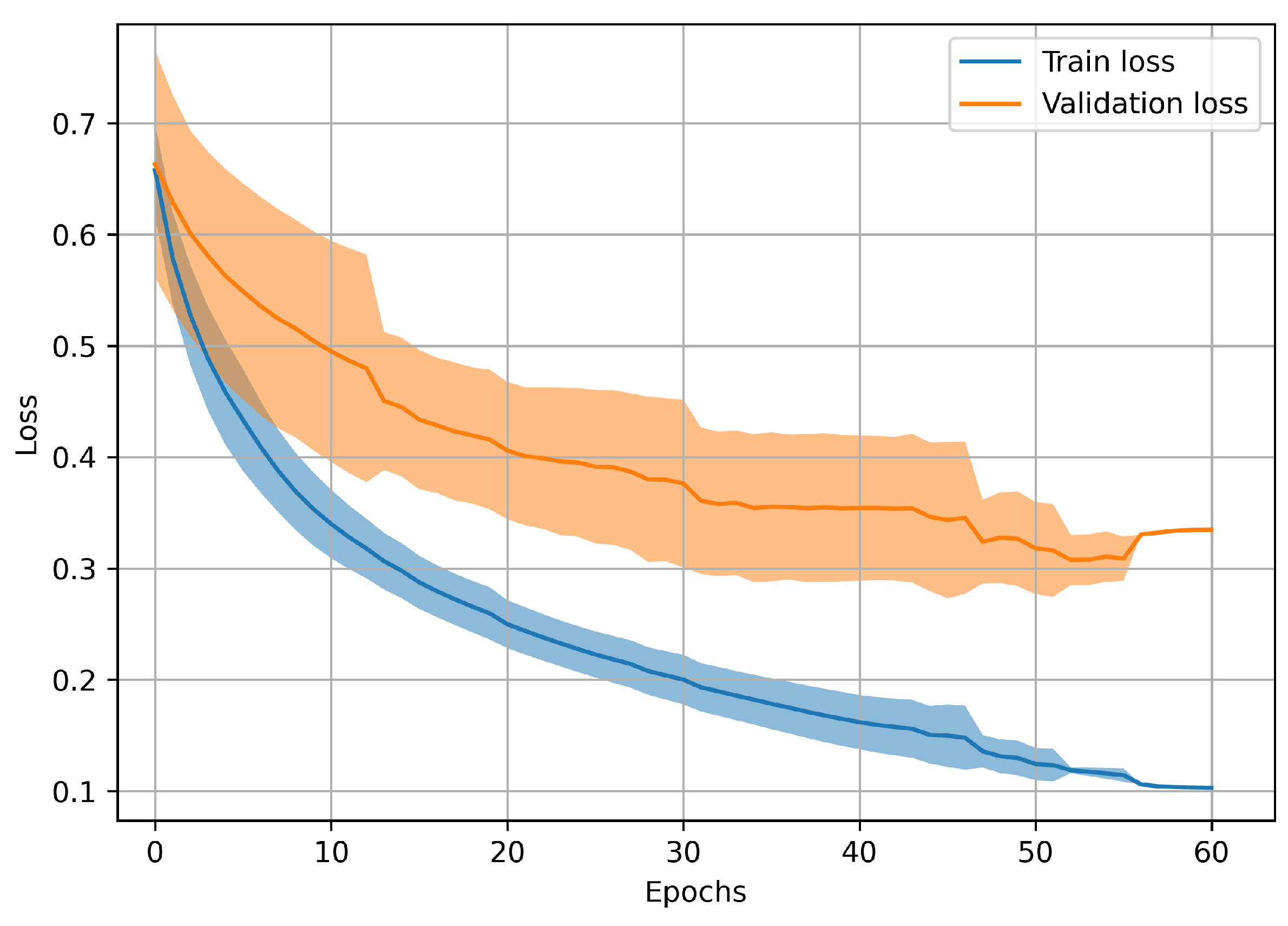
2.3.4. Training Stage

The purpose of using transfer learning focused on extracting the general knowledge of pattern recognition in ECG signals (cardiac cycles) and transfer that knowledge (e.g., high-level features) into IMU-based Human Activity tasks. That said, the training stage has been divided into three steps:
  • Train the Hourglass-shape CNN with clinical signals (ECG): this step is similar to that presented in the previous experiment, where the same architecture was trained with ECG signals from LUDB dataset;
  • Train the new architecture, adapted to multivariate data: in this step, the new network has been trained with the new target dataset (IMU data), with a frozen pre-trained block and both convolutional and decision-making trainable blocks;
  • Fine-tuning: all the network weights were unfrozen and training was applied in the same set but with a much lower learning rate during a small number of epochs.
Table 5 displays the hyperparameter settings employed on these three training steps.
After training, the model was capable of processing new activity signals. As the output consisted of a point-by-point output mask, it might not always be composed of well-defined windows (output smoothness). Hence, as a post-processing step, gaps were closed and short windows rejected if their length was lower than K and M points, respectively. In our case, K and M were both set to 10 points (representing 15 s with the chosen sampling rate).

2.3.5. Baseline Model Parameters

In this case, the multivariate version of sDTW has been employed to evaluate the multivariate IMU signals. As done in the previous experiment (with univariate time series), Table 6 presents the hyperparameters set out, regarding these Human Activity work cycle patterns.

2.4. Evaluation

Since the developed segmentation model is a point-by-point classifier, a standard evaluation might lead to a misinterpretation of the output, since point-by-point metrics (e.g., accuracy) might return high scores even when the segmentation performance is poor (misalignments and a few wrongly predicted cycles might not be enough to influence such scores). Instead, a cycle-by-cycle evaluation has been idealized as an adequate choice. Thus, a novel set of metrics is proposed and summarized in Figure 16, based on some time series and image segmentation concepts [50]. Each metric is, then, described in more detail, downstream:
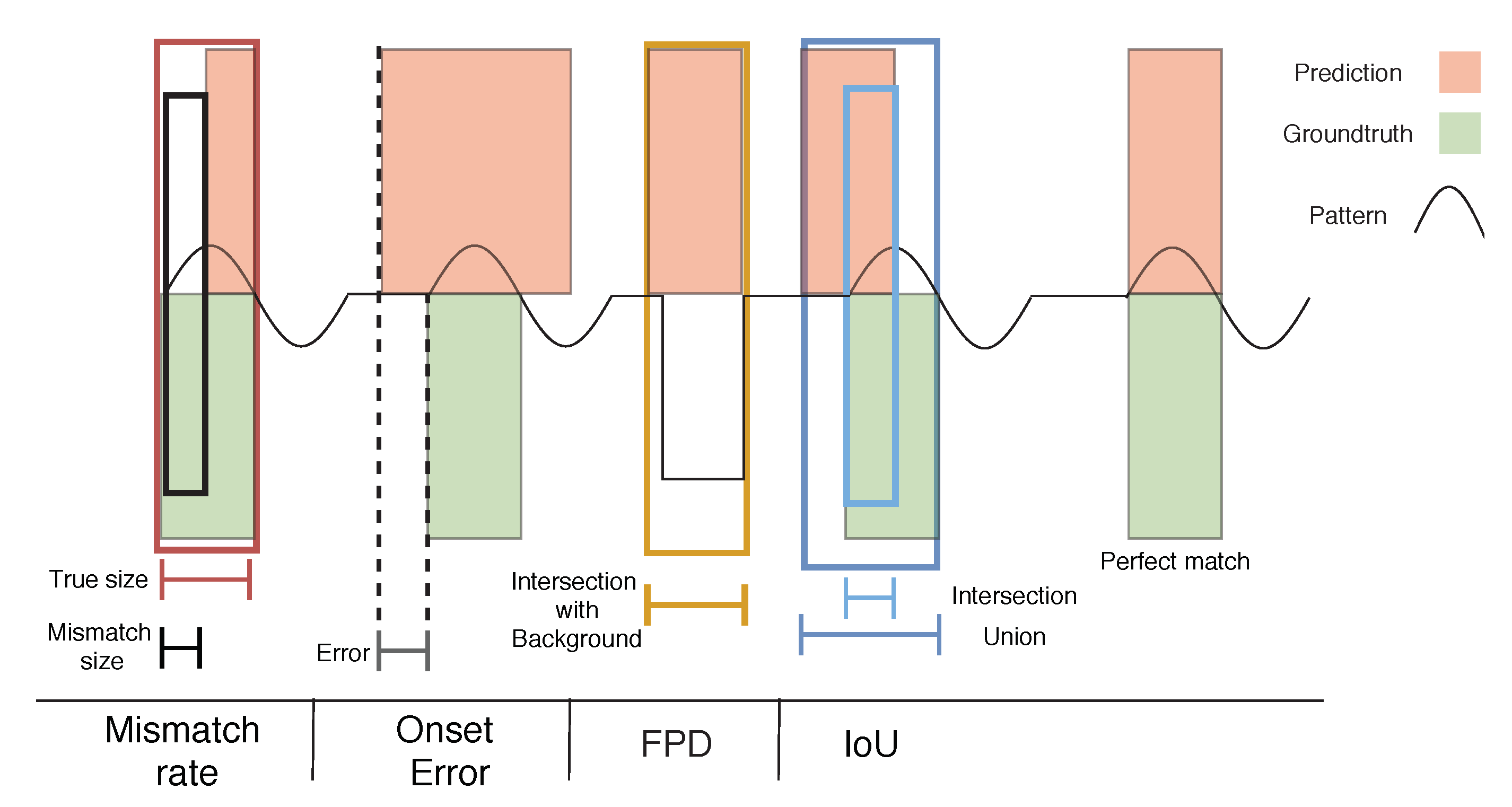
  • Intersection-over-Union (IoU): also known as the Jaccard coefficient [51], it computes the ratio between the number of matching points of both true and predicted cycles (Intersection) and the number of points both cycles fill in the whole signal (Union). Cycle patterns achieving an IoU greater than 0.44 (chosen empirically in preliminary experiments) are classified as True Positives (TP);
    IoU = I n t e r s e c t e d p o i n t s G r o u n d t r u t h p o i n t s + P r e d i c t e d p o i n t s I n t e r s e c t e d p o i n t s
  • False Positive Detection (FPD): The intersection of each predicted cycle with the Background mask (normalized by the cycle length) is performed. Those having an FPD above 0.80 (chosen empirically in preliminary experiments) are labeled as False Positives (FP);
    FPD = P r e d i c t e d m a s k · B a c k g r o u n d m a s k | P r e d i c t e d m a s k |
  • Precision and Recall: from the two previous scores, Precision and Recall metrics are easily calculated. As IoU and FPD scores return the number of TP and FP cycles, respectively, these metrics are computed as follows:
    Precision = TP TP + FP
    Recall = TP E x p e c t e d c y c l e s
  • Mismatch Rate (MR): it represents the percentage of wrongly annotated points within each true cycle;
    MR = M i s m a t c h p o i n t s G r o u n d t r u t h p o i n t s × 100 %
  • Onset/Offset error: it measures the temporal distance between predicted and real cycles onset and offset points (error), a good indicator to confirm the quality of the alignment;
  • Number of cycles: it compares the number of predicted and real cycles, being an additional high-level evaluation, as it is a metric of interest in such applications (e.g., for productivity measures).

3. Experimental Results

This section presents the obtained results concerning both univariate and multivariate described applications.

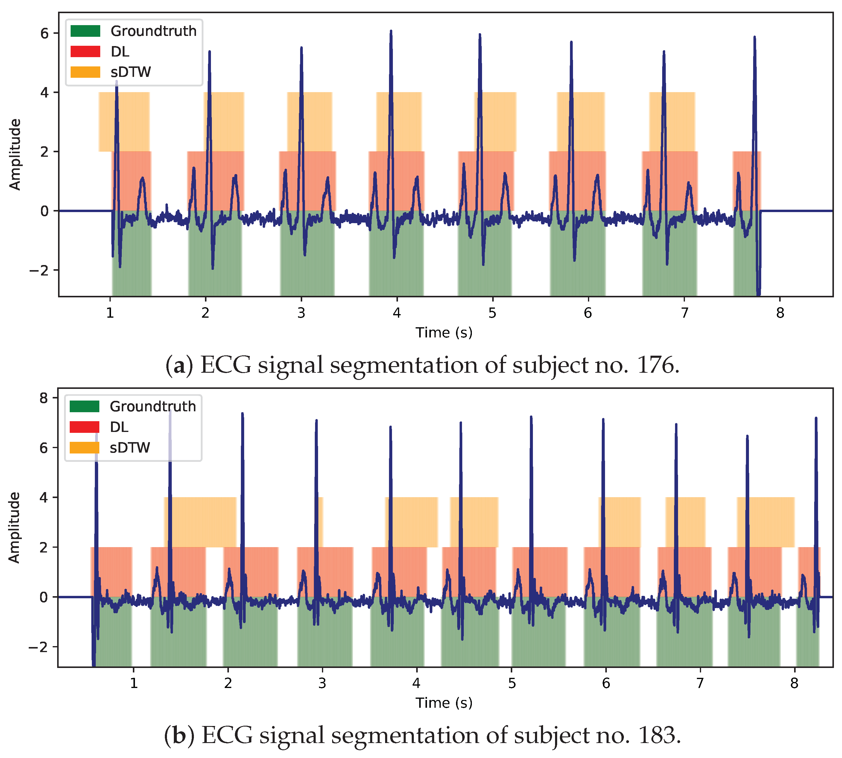
3.1. Univariate Analysis

The proposed conventional approach (sDTW model) required a reference template to perform the subsequence matching alignment. In this case, the template (Figure 17) has been chosen (by hand) as a proper representative of a normal cardiac cycle in ECG lead II.
The sDTW technique does not involve a training stage (as the proposed DL network), relying on subsequence matching, so it becomes a lot easier to obtain reproducible results. An example of the resulting paths in an ECG signal subsequence matching is shown in Figure 18.
Regarding the DL-based proposal, the training stage has stopped after 25 epochs, when validation loss started to stabilize and training loss kept decreasing (Figure 19). Following the loss progression trend, it suggests that training with even more epochs would increase the discrepancy between validation and training losses, which could induce model overfitting.
Regarding the segmentation performance of both approaches, visual examples of ECG signal segmentation from two different testing individuals are presented in Figure 20.
With reference to Figure 20a,b, the proposed DL approach shows it is capable of fitting adequately its predictions to the expected windows, likely because it undergoes a learning process (unlike sDTW) based on recognizing patterns in long sequences, making it skilled to handle signal variability better. The proposed NN was idealized to be learning the most general behavior of an ECG signal, such as the cardiac cycle general shape, its acceptable variability (including noise level), its recurrent periodicity, the typical types of background, among other attributes (extracted from the first convolutional layers). These insights might have been automatically acquired by the network layers (without the need of defining a reference template), revealing to be, at least in this case, more relevant than distance-based techniques (sDTW).
In Figure 20b, the high-frequency noise component seems to have little or no influence on the Hourglass CNN segmentation performance, meaning it is capable of ignoring that irrelevant element. In contrast, paths predicted by sDTW are somewhat dephased (or even absent), implying it might not perform correctly when dealing with noisy ECG sequences. In noiseless signals (Figure 20a) where complexes are well amplified, both approaches seem to match cardiac cycle windows adequately, despite the DL model’s predictions are better aligned with the ground truth windows.
In order to confirm the visual inferences drawn from the previous images, Table 7 presents an objective comparison, through the computation of previously described metrics across testing set signals, between the two models. We trained the Hourglass CNN model 15 distinct times (with 15 randomly sampled splits) to achieve a fair evaluation of the model’s performance with different train/validation/test sets, and averaged the results over these different training stages.
The overall metrics presented in Table 7 help demonstrate the greater performance of the Hourglass CNN model compared to the sDTW technique. Even though the cycle counting (P/T ratio) and the presence of false positive cycles (Precision) did not reveal huge discrepancies across approaches, the remaining metrics, that enhance the quality of the matching process (i.e., how well predicted windows fit the expected ones), showed a substantial contrast, quantitatively supporting that the DL-based model outputs/predicts more reliable cycle windows.

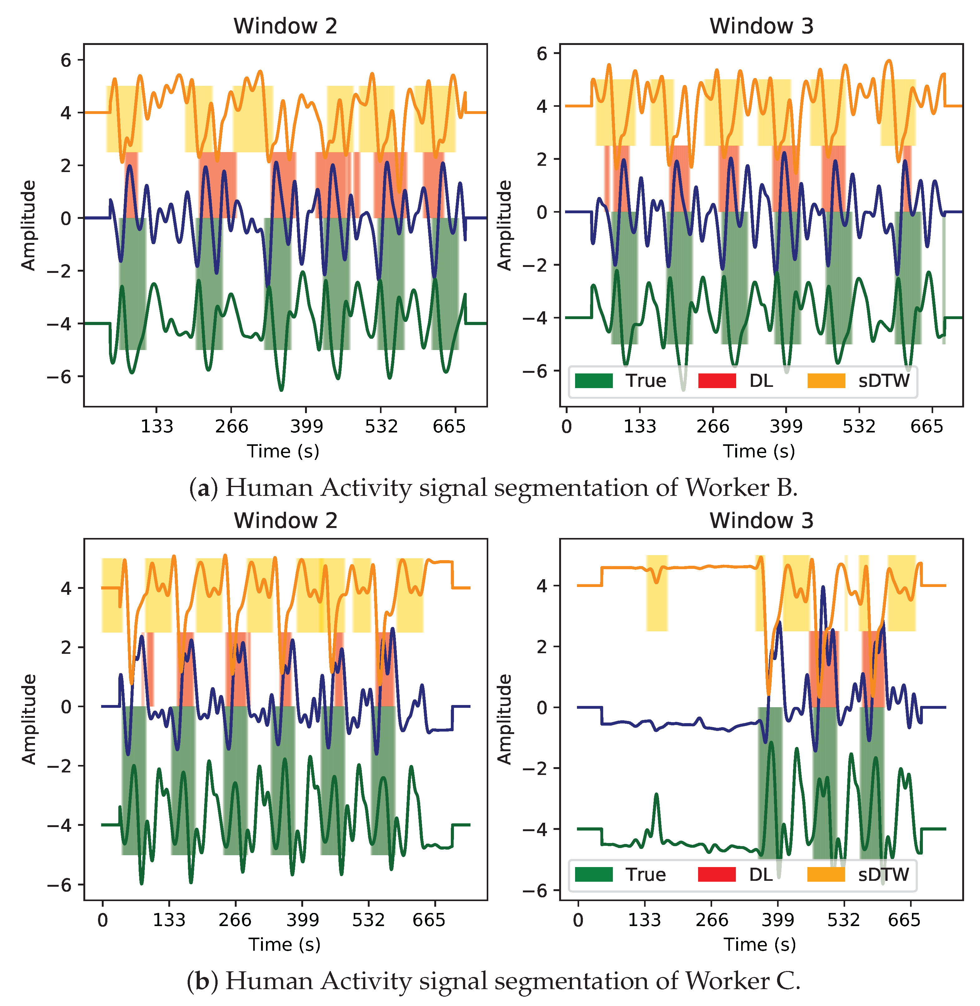
3.2. Multivariate Analysis

At this stage, inertial sensor-based Human Activity has been evaluated by the same two approaches, which suffered slight changes.
Regarding the sDTW technique, we adopted its multidimensional version, which enables the input of multivariate time series. This way, 3-dimensional sequences were evaluated in the context of industrial operators’ work cycles segmentation. Figure 21 presents a visual example of sDTW selected paths, regarding an activity executed by a single worker. The reference template has been chosen as a representative pattern of each activity and sensor (usually the less distorted and noisy activity cycle).
Concerning the multivariate-adapted Hourglass CNN model, the introduction of a transfer learning approach led to a training stage comprised of three distinct steps.
The first step involved training the Hourglass-shaped CNN with ECG signals, so that it learned to extract general temporal pattern features from more abundant cardiac cycles.
Before starting to describe the transfer learning training performance (last two steps), the impact of the augmentation employment on the model loss progression is shown in Figure 22. It seems clear that the application of data augmentation led to faster and better training/validation loss convergence.
In the second step, the pre-trained block has been frozen (non-trainable weights), while the convolutional block remained trainable and new decision layers were initialized (for each time series input channel) with random weights. This allowed reducing the number of trainable parameters, an important step to avoid overfitting issues. At this step, the number of trainable and non-trainable parameters were 171,532 and 51,696, respectively. The last training step consisted of unfreezing the pre-trained block weights so that they could be fine-tuned (with a much lower learning rate) to the domain of study (Human Activity).
Relative to the loss progressions, since a leave-one-worker-out scheme has been followed, several complete training stages were required. In this sense, Figure 23 displays the loss progression together with the variability associated with each epoch.
Observing Figure 23, all the procedures executed to improve the model training (essentially data augmentation, train early stopping, transfer learning from ECG domain) led to the desired loss progression, characterized by a validation loss trend which follows the training one (without rising), even though it does never reach the latter.
In an attempt of evaluating and comparing each method in a multivariate pattern segmentation context, the following discussion is supported by human activity segmentation images regarding workers with the same sensor placement and performing the same activity so that intra- and inter-subject pattern variability becomes an element for describing each model ability to detect new patterns from the learned ones.
In Figure 24, the presented segmentation is shown in two of the three independent workers’ signals, acquired during Fender activity execution and monitored on their wrist IMU sensor.
The first visual impressions suggest that the multivariate work cycles contain an evident morphological variability between these two workers. Although there is a standard work method, there is also some variability among the operators since slight variations in the work method might exist. Every so often, searching for cyclic patterns (even visually) might be complex, making this segmentation task more challenging (in comparison to ECG patterns). This statement is reflected in Worker B signals (Figure 24a), whose patterns do not show a relevant amplitude contrast relative to the signal baseline, possibly due to either an inappropriate activity execution or signal corruption with another type of movement (or even acquisition noise). In contrast, Worker C signals (Figure 24b) produce an easier pattern to recognize visually.
Even though both models (DL and sDTW) contain some sporadic misclassified patterns, they present good results at detecting each worker’s activity cycles, effectively dealing with several variability components. Through visual inference, it seems the DL network is capable of better adjusting its predicted windows to the expected work cycle windows than sDTW. Additionally, the conventional approach also fails at detecting some cycle regions that the DL model fits adequately well (especially in Figure 24b).
As done previously, such visual interpretations were further confirmed through quantitative analysis, performed through the aforementioned set of segmentation metrics. Such obtained metrics were averaged per each activity/sensor pair and are presented in Table 8.
Firstly, we note those scores are relatively worse when compared with the experiment with ECG data, which indicates how complex this problem is. The degree of variability found in Human Activity IMU-based time series is far greater than in the ECG domain, so the decrease in performance was somewhat expected.
Regarding the P/T ratio metric, the scores are similar for both models over all the activity/sensor pairs, although the DL model achieves better scores for the Fender activity and the sDTW technique for the Liftgate one. Nevertheless, all values are close to 1, indicating the number of counted cycles does not suffer a considerable deviation from the real one.
With respect to the Precision metric, again, the DL model performance generally surpassed that of the sDTW, even though scores are not too discrepant. Overall, precision scores ranged from 66.67% to 83.08%, in DL, and from 33.15% to 77.20% in sDTW, meaning the latter possesses a higher proportion of FP cycles over its set of predictions.
In terms of Recall, the DL approach has performed better than sDTW in all four activities, meaning the proposed technique generates the most suitable windows (with greater IoU scores), with respect to the expected work cycle windows. Scores ranged from 62.52% to 82.59% in DL, and from 26.24% to 71.97% in sDTW.
Mismatch-Rate scores come in the same reasoning path, confirming the DL technique predicted cycle windows tend to be less dephased from the truth windows, with greater IoU values and a lower percentage of missing cycle points (mismatch).
Observing the temporal errors, the overall scores suggest better performance on the sDTW side (lower errors) in the majority of the activities, which can be misleading given the results of the previous metrics. For instance, in Fender-Chest and Liftgate-Wrist signals, the sDTW technique achieved lower Onset/Offset errors associated with worse Recall (lower) and MR (higher) scores than the DL model. Although it seems discordant, the DL predicted cycles can be larger and cover a greater proportion of the cycle but be dephased (or overflow the true cycle borders), filling also part of the background content, while sDTW cycles can be shorter and inserted within the true cycle region. In such cases, inner shorter windows will tend to have a lower IoU (low intersection), a high MR, but lower errors. Larger dephased windows will return the opposite. The remaining two activities (Fender-Wrist and Liftgate-Elbow) show better performances from the proposed neural network model (DL).
In summary, as for the ECG application, the results support a better segmentation performance by the proposed DL-based approach. The fact the implemented architecture gained the ability to extract relevant features from each channel has revealed noticeable benefits when it comes to detecting activity patterns within multivariate signals, even with low data availability. At the same time, this reasonable performance must not be misled by the achievement of generalization. In fact, the reduced amount of signals (within each worker) and the lack of inter-worker variability (few workers for a given task) do not make the work cycle pattern generalization possible for all the subjects performing that task. Furthermore, any judgement under the scope of these results should not be supported by absolute statements, since they would need further validation (with a greater amount and other types of data). In any case, the application of transfer learning from ECG signals to the Human Activity domain has shown great potential even with dataset size concerns and more complex segmentation tasks.

4. Conclusions

In this paper, a new Deep Learning approach has been proposed to improve the segmentation of patterns in time series, aiming to increase the robustness of the matching process, flexibly handling natural variability issues of such signals. The application of the proposed model was shown in two distinct domains. The first is related to the segmentation of cardiac cycles in ECG time series data, where training data is abundant, whereas the second application concerned IMU-based Human Activity signals, where data was much scarcer. Nonetheless, we proposed to follow a Transfer Learning approach to achieve domain adaptation, shown to be successful, even with minimal data samples in the target domain.
The proposed architecture was a Convolution/Deconvolution NN (named Hourglass CNN), idealized to execute Univariate and Multivariate time series pattern segmentation. As template-based segmentation approaches are more abundant in the literature, those have supported the discussion of the DL model performance. Thus, a conventional approach was defined as a baseline for performance comparison purposes: sDTW, a template-based subsequence matching algorithm.
The goal of this experiment consisted of detecting similar matches of a particular pattern category in long signals. The univariate analysis has been conducted in ECG signals from the LUDB dataset. Visually, cardiac cycle occurrence sites predicted by the proposed model were reasonably fitted to the expected ones, even evaluating ECG signals with increased noise components, which must be highlighted. Objectively, the DL-based model expressed greater scores than those obtained by the sDTW technique.
The multivariate analysis was performed in IMU data extracted from a Human Activity dataset. The collection and processing of human movement data in manufacturing sites offer faster, accurate, and ubiquitous digitalization, which helps analyze and improve manufacturing and assembly line processes. The collected information may be used to oversee task execution by the worker and implement pedagogical strategies to refrain workers from performing incorrect movements or adapt different strategies to improve well-being.
This problem was more challenging for several reasons: The multi-dimensionality of data, the relevant morphological variability of activity patterns compared to that of heartbeats, and the lack of signals. The latter issue led to the application of a transfer learning approach and data augmentation techniques, preventing network overfitting. By visual observation of the data, the proposed DL model segmentation still achieved an adequate performance, although relatively worse when compared to the aforementioned in cardiac cycles. However, the scores were still considerably better than those obtained by the sDTW technique, which favors the robustness of a learning-based segmentation method.
Furthermore, although it has not been quantitatively validated, in terms of temporal complexity, the inference step of the proposed model is expected to be faster than that of sDTW algorithm by the fact the latter requires the computation of a cost matrix and a path searching method every time a new sequence is evaluated (although it does not require a training stage), while the former only needs a set of tuned weights.
Regarding some future work guidelines, posterior analysis could use the annotated pattern cycles (from ground truth) in a metric learning approach for measuring the similarity of each predicted pattern, constituting an additional filter to mitigate the presence of wrongly annotated windows. Another option could consist of implementing a Variational Autoencoder (VAE) model so that it learns the general shape of annotated patterns, being, then, able to reject some wrongly predicted ones, regarding an eventual real-world application. The addition of more types of background (instead of exclusively the baseline between consecutive cycles) such as noise, artifacts, and out-of-domain signals would also help to increase the generalization capacity of the proposed network. Apart from that, performing this analysis in additional datasets and other data types (even outside the physiological/human activity domains) would help validate this pipeline and consolidate the results obtained and reported in this paper. Additional datasets such as the MIT-BIH Arrhythmia (ECG signals) [52] and Fantasia (ECG and Respiration time series) [53] datasets could be a suitable alternative to test the transfer learning hypothesis from biosignals to IMU-based pattern segmentation. The evaluation of the segmentation performance on other types of biosignals such as the EEG (e.g., from the S-EDF-153 [54] dataset) could also comprise an interesting experiment regarding a deeper validation of the proposed framework. With respect to other IMU-based human activity datasets, the AnDy [55] dataset should also be considered as an appropriate option.

Author Contributions

Conceptualization, P.M. and A.C.; Data curation, P.M. and D.F.; Formal analysis, P.M., D.F. and A.C.; Methodology, P.M. and A.C.; Project administration, H.G.; Supervision, D.F., H.G. and A.C.; Writing—original draft, P.M.; Writing—review & editing, P.M., D.F., H.G. and A.C. All authors have read and agreed to the published version of the manuscript.

Funding

Project OPERATOR (NORTE-01-0247-FEDER-045910) leading to this work is co-financed by the ERDF - European Regional Development Fund through the North Portugal Regional Operational Program and Lisbon Regional Operational Program and by the Portuguese Foundation for Science and Technology, under the MIT Portugal Program (2019 Open Call for Flagship projects).

Data Availability Statement

The LUDB Dataset is publicly available at LUDB (https://physionet.org/content/ludb/1.0.1). The human activity dataset is private, and thus cannot be publicly released.

Conflicts of Interest

The authors declare no conflict of interest.

Appendix A. Supplementary Details about the Neural Network Architecture Choice

Some similar papers (referenced in Section 1.3), published by Sereda et al. [16] and Moskalenko et al. [35], have tested their networks’ performance in LUDB dataset, although considering a multi-classification task (distinguishing P, QRS, T waveforms, and the signal background). The segmentation metrics were proposed in [16], being available on Github (https://github.com/Namenaro/ecg_segmentation/blob/master/metrics.py, accessed on 21 March 2021). Such metrics measure how (temporally) close each predicted ECG wave’s onset and offset timestamp is from the expected, using a tolerance parameter that defines which annotations are close enough (True Positive—TP) and whose are outside that tolerance interval (False Positives—FP). Note the concept of TP and FP is different than the described in this paper.
Table A1. Overview of the segmentation performance metrics across the proposed architecture and two already proposed in the literature. Error distributions are presented as the averaged temporal errors and the corresponding standard deviation. Best scores are highlighted.
MetricModelEvaluated ECG Segment
P onset P offset QRS onset QRS offset T onset T offset
Sensitivity (%) HG100.0100.0100.0100.099.798.8
C/D99.699.6100.0100.097.097.0
U-Net96.296.299.799.799.197.6
Precision (%) HG90.790.798.488.191.990.8
C/D89.789.798.287.893.393.0
U-Net92.392.399.799.495.994.2
Error distribution
( μ ± σ m s )
HG−1.8 ± 18.3−3.7 ± 15.61.3 ± 9.4−0.9 ± 11.3−5.1 ± 32.7−3.4 ± 28.3
C/D1.2 ± 19.2−4.4 ± 17.61.3 ± 10.32.0 ± 11.3−2.9 ± 30.11.5 ± 29.8
U-Net−1.0 ± 11.8−4.7 ± 14.70.1 ± 11.11.4 ± 10.6−10.0 ± 35.0−13.0 ± 33.0
HG—Hourglass architecture (Ours); C/D—Sequential Convolution/Deconvolution architecture [16]; U-Net—U-shaped architecture [35].

References

  1. Demrozi, F.; Pravadelli, G.; Bihorac, A.; Rashidi, P. Human Activity Recognition using Inertial, Physiological and Environmental Sensors: A Comprehensive Survey. IEEE Access 2020, 8, 210816–210836. [Google Scholar] [CrossRef]
  2. Lin, J.; Williamson, S.; Borne, K.; DeBarr, D. Pattern Recognition in Time Series. 2011. Available online: https://cs.gmu.edu/~jessica/publications/astronomy11.pdf (accessed on 23 January 2021).
  3. Fong, S.; Lan, K.; Sun, P.; Mohammed, S.; Fiaidhi, J. A Time-Series Pre-Processing Methodology for Biosignal Classification using Statistical Feature Extraction. In Proceedings of the 10th IASTED International Conference on Biomedical Engineering (Biomed’13), Innsbruck, Austria, 11–13 February 2013. [Google Scholar] [CrossRef] [Green Version]
  4. Folgado, D.; Barandas, M.; Matias, R.; Martins, R.; Carvalho, M.; Gamboa, H. Time Alignment Measurement for Time Series. Pattern Recognit. 2018, 81, 268–279. [Google Scholar] [CrossRef]
  5. Rodpongpun, S.; Niennattrakul, V.; Ratanamahatana, C. Efficient Subsequence Search on Streaming Data Based on Time Warping Distance. ECTI Trans. Comput. Inf. Technol. 2011, 5, 2–8. [Google Scholar] [CrossRef]
  6. Osowski, S.; Tran, L. ECG Beat Recognition Using Fuzzy Hybrid Neural Network. Biomed. Eng. IEEE Trans. 2001, 48, 1265–1271. [Google Scholar] [CrossRef]
  7. Deppe, S.; Lohweg, V. Survey on time series motif discovery: Time series motif discovery. Wiley Interdiscip. Rev. Data Min. Knowl. Discov. 2017, 7, e1199. [Google Scholar] [CrossRef]
  8. Miao, S.; Vespier, U.; Cachucho, R.; Meeng, M.; Knobbe, A. Predefined pattern detection in large time series. Inf. Sci. 2016, 329, 950–964. [Google Scholar] [CrossRef] [Green Version]
  9. Acharya, U.R.; Oh, S.L.; Hagiwara, Y.; Tan, J.H.; Adam, M.; Gertych, A.; San Tan, R. A Deep Convolutional Neural Network Model to Classify Heartbeats. Comput. Biol. Med. 2017, 89, 389–396. [Google Scholar] [CrossRef]
  10. Piacentino, E.; Guarner, A.; Angulo, C. Generating Synthetic ECGs Using GANs for Anonymizing Healthcare Data. Electronics 2021, 10, 389. [Google Scholar] [CrossRef]
  11. Deng, L.; Jaitly, N. Deep Discriminative and Generative Models for Speech Pattern Recognition. In Handbook of Pattern Recognition and Computer Vision (Ed. C.H. Chen); World Scientific: Singapore, 2016; pp. 27–52. [Google Scholar]
  12. Zhao, B.; Lu, H.; Chen, S.; Liu, J.; Wu, D. Convolutional neural networks for time series classification. J. Syst. Eng. Electron. 2017, 28, 162–169. [Google Scholar] [CrossRef]
  13. Salehinejad, H.; Sankar, S.; Barfett, J.; Colak, E.; Valaee, S. Recent Advances in Recurrent Neural Networks. arXiv 2018, arXiv:1801.01078. [Google Scholar]
  14. Graves, A.; Mohamed, A.; Hinton, G. Speech recognition with deep recurrent neural networks. In Proceedings of the 2013 IEEE International Conference on Acoustics, Speech and Signal Processing, Vancouver, BC, Canada, 26–30 May 2013; pp. 6645–6649. [Google Scholar] [CrossRef] [Green Version]
  15. Kasfi, K.T.; Hellicar, A.; Rahman, A. Convolutional Neural Network for Time Series Cattle Behaviour Classification. In Proceedings of the Workshop on Time Series Analytics and Applications; Association for Computing Machinery: New York, NY, USA, 2016; pp. 8–12. [Google Scholar] [CrossRef]
  16. Sereda, I.; Alekseev, S.; Koneva, A.; Kataev, R.; Osipov, G. ECG Segmentation by Neural Networks: Errors and Correction. arXiv 2018, arXiv:1812.10386. [Google Scholar]
  17. Cassisi, C.; Montalto, P.; Aliotta, M.; Cannata, A.; Pulvirenti, A. Similarity Measures and Dimensionality Reduction Techniques for Time Series Data Mining. In Advances in Data Mining Knowledge Discovery and Applications; Karahoca, A., Ed.; IntechOpen: Rijeka, Croatia, 2012; Chapter 3. [Google Scholar] [CrossRef] [Green Version]
  18. Zhang, Z.; Jiang, J.; Liu, X.; Lau, R.; Wang, H.; Zhang, R. A Real Time Hybrid Pattern Matching Scheme for Stock Time Series. Conf. Res. Pract. Inf. Technol. Ser. 2010, 104, 161–170. [Google Scholar]
  19. Tsinaslanidis, P.E.; Zapranis, A.D. Dynamic Time Warping for Pattern Recognition. In Technical Analysis for Algorithmic Pattern Recognition; Springer International Publishing: Berlin/Heidelberg, Germany, 2016; pp. 193–204. [Google Scholar] [CrossRef]
  20. Santos, A.; Rodrigues, J.; Folgado, D.; Santos, S.; Fujão, C.; Gamboa, H. Self-Similarity Matrix of Morphological Features for Motion Data Analysis in Manufacturing Scenarios. In Proceedings of the 14th International Joint Conference on Biomedical Engineering Systems and Technologies—BIOSIGNALS, INSTICC; SciTePress: Setubal, Portugal, 2021; pp. 80–90. [Google Scholar] [CrossRef]
  21. Nguyen-Dinh, L.V.; Roggen, D.; Calatroni, A.; Tröster, G. Improving Online Gesture Recognition with Template Matching Methods in Accelerometer Data. In Proceedings of the 12th International Conference on Intelligent Systems Design and Applications (ISDA), Kochi, India, 27–29 November 2012. [Google Scholar] [CrossRef]
  22. Barth, J.; Oberndorfer, C.; Kugler, P.; Schuldhaus, D.; Winkler, J.; Klucken, J.; Eskofier, B. Subsequence dynamic time warping as a method for robust step segmentation using gyroscope signals of daily life activities. In Proceedings of the 2013 35th Annual International Conference of the IEEE Engineering in Medicine and Biology Society (EMBC), Osaka, Japan, 3–7 July 2013; pp. 6744–6747. [Google Scholar] [CrossRef]
  23. Gong, Z.; Chen, H. Dynamic State Warping. arXiv 2017, arXiv:1703.01141. [Google Scholar]
  24. Barandas, M.; Folgado, D.; Fernandes, L.; Santos, S.; Abreu, M.; Bota, P.; Liu, H.; Schultz, T.; Gamboa, H. TSFEL: Time Series Feature Extraction Library. SoftwareX 2020, 11, 100456. [Google Scholar] [CrossRef]
  25. Bota, P.; Silva, J.; Folgado, D.; Gamboa, H. A Semi-Automatic Annotation Approach for Human Activity Recognition. Sensors 2019, 19, 501. [Google Scholar] [CrossRef] [PubMed] [Green Version]
  26. Matias, P.; Folgado, D.; Gamboa, H.; Carreiro, A. Robust Anomaly Detection in Time Series through Variational AutoEncoders and a Local Similarity Score. In Proceedings of the 14th International Joint Conference on Biomedical Engineering Systems and Technologies—BIOSIGNALS, INSTICC; SciTePress: Setubal, Portugal, 2021; pp. 91–102. [Google Scholar] [CrossRef]
  27. Mekruksavanich, S.; Jitpattanakul, A. Biometric User Identification Based on Human Activity Recognition Using Wearable Sensors: An Experiment Using Deep Learning Models. Electronics 2021, 10, 308. [Google Scholar] [CrossRef]
  28. Avanzato, R.; Beritelli, F. Automatic ECG Diagnosis Using Convolutional Neural Network. Electronics 2020, 9, 951. [Google Scholar] [CrossRef]
  29. Kłosowski, G.; Rymarczyk, T.; Wójcik, D.; Skowron, S.; Cieplak, T.; Adamkiewicz, P. The Use of Time-Frequency Moments as Inputs of LSTM Network for ECG Signal Classification. Electronics 2020, 9, 1452. [Google Scholar] [CrossRef]
  30. Nurmaini, S.; Darmawahyuni, A.; Sakti Mukti, A.N.; Rachmatullah, M.N.; Firdaus, F.; Tutuko, B. Deep Learning-Based Stacked Denoising and Autoencoder for ECG Heartbeat Classification. Electronics 2020, 9, 135. [Google Scholar] [CrossRef] [Green Version]
  31. Krizhevsky, A.; Sutskever, I.; Hinton, G.E. ImageNet Classification with Deep Convolutional Neural Networks. In Advances in Neural Information Processing Systems; Curran Associates, Inc.: New York, NY, USA, 2012; Volume 25, pp. 1097–1105. [Google Scholar]
  32. Gamboa, J.C.B. Deep Learning for Time-Series Analysis. arXiv 2017, arXiv:1701.01887. [Google Scholar]
  33. Nanni, L.; Ghidoni, S.; Brahnam, S. Handcrafted vs. Non-Handcrafted Features for computer vision classification. Pattern Recognit. 2017, 71, 158–172. [Google Scholar] [CrossRef]
  34. Perslev, M.; Jensen, M.H.; Darkner, S.; Jennum, P.J.; Igel, C. U-Time: A Fully Convolutional Network for Time Series Segmentation Applied to Sleep Staging. arXiv 2019, arXiv:1910.11162. [Google Scholar]
  35. Moskalenko, V.; Zolotykh, N.; Osipov, G. Deep Learning for ECG Segmentation. Adv. Neural Comput. Mach. Learn. Cogn. Res. III 2019, 856, 246–254. [Google Scholar] [CrossRef] [Green Version]
  36. Kuederle, A. sDTW Multi Path Matching. Available online: https://tslearn.readthedocs.io/en/stable/auto_examples/metrics/plot_sdtw.html (accessed on 28 July 2020).
  37. Müller, M. Dynamic time warping. Inf. Retr. Music. Motion 2007, 2, 69–84. [Google Scholar] [CrossRef]
  38. Hong, J.Y.; Park, S.H.; Baek, J.G. SSDTW: Shape segment dynamic time warping. Expert Syst. Appl. 2020, 150, 113291. [Google Scholar] [CrossRef]
  39. Jeong, Y.S.; Jeong, M.K.; Omitaomu, O.A. Weighted dynamic time warping for time series classification. Pattern Recognit. 2011, 44, 2231–2240. [Google Scholar] [CrossRef]
  40. Munich, M.; Perona, P. Continuous Dynamic Time Warping for translation-invariant curve alignment with applications to signature verification. In Proceedings of the Seventh IEEE International Conference on Computer Vision, Kerkyra, Greece, 20–27 September 1999; Volume 1. [Google Scholar] [CrossRef] [Green Version]
  41. Noh, H.; Hong, S.; Han, B. Learning Deconvolution Network for Semantic Segmentation. In Proceedings of the 2015 IEEE International Conference on Computer Vision (ICCV), Santiago, Chile, 7–13 December 2015; pp. 1520–1528. [Google Scholar] [CrossRef] [Green Version]
  42. Ioffe, S.; Szegedy, C. Batch Normalization: Accelerating Deep Network Training by Reducing Internal Covariate Shift. In Proceedings of the 32nd International Conference on Machine Learning; Bach, F., Blei, D., Eds.; PMLR: Lille, France, 2015; Volume 37, pp. 448–456. Available online: http://proceedings.mlr.press/v37/ioffe15.html (accessed on 21 June 2020).
  43. Kalyakulina, A.I.; Yusipov, I.I.; Moskalenko, V.A.; Nikolskiy, A.V.; Kosonogov, K.A.; Osipov, G.V.; Zolotykh, N.Y.; Ivanchenko, M.V. LUDB: A New Open-Access Validation Tool for Electrocardiogram Delineation Algorithms. IEEE Access 2020, 8, 186181–186190. [Google Scholar] [CrossRef]
  44. Luz, E.J.; Schwartz, W.R.; Cámara-Chávez, G.; Menotti, D. ECG-based heartbeat classification for arrhythmia detection: A survey. Comput. Methods Programs Biomed. 2016, 127, 144–164. [Google Scholar] [CrossRef]
  45. De Chazal, P.; O’Dwyer, M.; Reilly, R.B. Automatic classification of heartbeats using ECG morphology and heartbeat interval features. IEEE Trans. Biomed. Eng. 2004, 51, 1196–1206. [Google Scholar] [CrossRef] [Green Version]
  46. Tan, C.; Sun, F.; Kong, T.; Zhang, W.; Yang, C.; Liu, C. A Survey on Deep Transfer Learning. In Artificial Neural Networks and Machine Learning—ICANN 2018; Kůrková, V., Manolopoulos, Y., Hammer, B., Iliadis, L., Maglogiannis, I., Eds.; Springer International Publishing: Berlin/Heidelberg, Germany, 2018; pp. 270–279. [Google Scholar] [CrossRef] [Green Version]
  47. Santos, S.; Folgado, D.; Rodrigues, J.; Mollaei, N.; Fujão, C.; Gamboa, H. Explaining the Ergonomic Assessment of Human Movement in Industrial Contexts. In Proceedings of the 13th International Joint Conference on Biomedical Engineering Systems and Technologies, Valletta, Malta, 24–26 February 2020; Volume 4, pp. 79–88. [Google Scholar] [CrossRef]
  48. Elisseeff, A.; Pontil, M. Leave-one-out error and stability of learning algorithms with applications Stability of Randomized Learning Algorithms Source. Int. J. Syst. Sci. IJSySc 2002, 6, 1–12. Available online: https://www.math.arizona.edu/~hzhang/math574m/Read/LOOtheory.pdf (accessed on 23 June 2020).
  49. Wen, T. tsaug. 2019. Available online: https://tsaug.readthedocs.io/en/stable/ (accessed on 20 July 2020).
  50. van Beers, F.; Lindström, A.; Okafor, E.; Wiering, M. Deep Neural Networks with Intersection over Union Loss for Binary Image Segmentation. ICPRAM 2019, 438–445. [Google Scholar] [CrossRef]
  51. Güneş, I.; Gunduz Oguducu, S.; Cataltepe, Z. Link prediction using time series of neighborhood-based node similarity scores. Data Min. Knowl. Discov. 2015, 30, 147–180. [Google Scholar] [CrossRef]
  52. Moody, G.; Mark, R. The impact of the MIT-BIH Arrhythmia Database. IEEE Eng. Med. Biol. Mag. 2001, 20, 45–50. [Google Scholar] [CrossRef] [PubMed]
  53. Iyengar, N.; Peng, C.K.; Morin, R.; Goldberger, A.L.; Lipsitz, L.A. Age-related alterations in the fractal scaling of cardiac interbeat interval dynamics. Am. J. Physiol. Regul. Integr. Comp. Physiol. 1996, 271, R1078–R1084. [Google Scholar] [CrossRef] [PubMed] [Green Version]
  54. Kemp, B.; Zwinderman, A.; Tuk, B.; Kamphuisen, H.; Oberye, J. Analysis of a sleep-dependent neuronal feedback loop: The slow-wave microcontinuity of the EEG. IEEE Trans. Biomed. Eng. 2000, 47, 1185–1194. [Google Scholar] [CrossRef]
  55. Maurice, P.; Malaisé, A.; Amiot, C.; Paris, N.; Richard, G.J.; Rochel, O.; Ivaldi, S. Human movement and ergonomics: An industry-oriented dataset for collaborative robotics. Int. J. Robot. Res. 2019, 38, 1529–1537. [Google Scholar] [CrossRef]
Figure 1. Illustration of sliding window-based pattern searching method applied to an artificially generated signal.
Electronics 10 01805 g001
Figure 2. Illustration of several types of time series variability. Two similar patterns differ due to (A) noise corruption, (B) size scaling, (C) amplitude scaling, (D) time shifting. Reproduced from [7].
Electronics 10 01805 g002
Figure 3. Schematized CNN architecture. Reproduced from [15].
Electronics 10 01805 g003
Figure 4. Illustration example of a Convolution/Deconvolution Neural Network. Reproduced from [16].
Electronics 10 01805 g004
Figure 5. Illustration of sDTW multi-path searching method. Darker regions correspond to lower distances (higher similarity). The optimal alignment paths are represented in white.
Electronics 10 01805 g005
Figure 6. Illustration of the Hourglass CNN architecture.
Electronics 10 01805 g006
Figure 7. Schematic cardiac cycle and its annotated segments, in LUDB dataset. Reproduced from [43].
Electronics 10 01805 g007
Figure 8. Pre-processing steps applied on ECG signals. On top, the signal baseline extracted by both median filters is highlighted in red. Note both amplitude and time scales have changed, due to downsampling and standardization.
Electronics 10 01805 g008
Figure 9. Illustration of the Hourglass Neural Network architecture, for univariate signals, used to define the first training stage performed on ECG signals and to fine-tune on new domains.
Electronics 10 01805 g009
Figure 10. Illustration of the Hourglass Neural Network architecture, for multivariate signals. The number of added channels (CH) has no restrictions.
Electronics 10 01805 g010
Figure 11. IMU sensors placement over the worker’s arm. For each subject, four sensors are placed on their hand, wrist, elbow and chest. Reproduced from [47].
Electronics 10 01805 g011
Figure 12. Data filtered through a butterworth lowpass filter (0.05 Hz cut-off). The lightest color corresponds to the raw signal, and the darkest to the filtered one. Work cycle transitions are represented with a red vertical line. Signals refer to Liftgate activity, monitored with the Elbow sensor.
Electronics 10 01805 g012
Figure 13. Example of the downsampling transformation applied to human activity signals. Red vertical lines represent work cycles transitions. No distortion has been induced on work cycles shapes.
Electronics 10 01805 g013
Figure 14. Definition of the ground truth masks. Work cycle transition points are highlighted with red vertical lines and their corresponding patterns with green windows. Non-highlighted regions represent the signal background component.
Electronics 10 01805 g014
Figure 15. Example of augmentation techniques applied to activity signals. Timeline contraction and dilation, and the addition of Gaussian noise were the parameters changed to generate new artificial samples.
Electronics 10 01805 g015
Figure 16. Illustration of the proposed segmentation evaluation metrics on an artificially generated signal. The metrics depicted are the Mismatch Rate (MR), Onset error, False Positive Detection (FPD), and Intersection over Union (IoU).
Electronics 10 01805 g016
Figure 17. Illustration of the defined representative template of lead II ECG signals.
Electronics 10 01805 g017
Figure 18. Illustration of the set of paths obtained after applying the sDTW algorithm to an ECG signal. Darker and lighter pixels represent lower and higher distances, respectively. White paths correspond to optimal subsequence alignments.
Electronics 10 01805 g018
Figure 19. Hourglass CNN training and validation loss progression, during training.
Electronics 10 01805 g019
Figure 20. Segmentation performance comparison between Houglass CNN (DL) and sDTW, regarding ECG signals of two different subjects present in the testing set.
Electronics 10 01805 g020
Figure 21. Illustration of the obtained paths after the sDTW algorithm application to a Liftgate activity signal, extracted from Worker A elbow IMU sensor. Note the three axis were averaged and compressed into a single one to facilitate the paths visual correspondence.
Electronics 10 01805 g021
Figure 22. Example of loss progressions of the same proposed NN, trained with (72 samples) and without (9 samples) augmented samples.
Electronics 10 01805 g022
Figure 23. Evolution of the network training and validation losses over the epochs. The darker line represents the average ( μ ) loss over all the training stages, while the lighter regions show the associated standard deviation ( σ ) surrounding the mean trend ( L o s s = μ ± σ ).
Electronics 10 01805 g023
Figure 24. Segmentation performance comparison between Houglass CNN (DL) and sDTW of Fender activity signals collected with the wrist sensor. Accelerometer x, y and z axes are represented by blue, orange, and green signals, correspondingly.
Electronics 10 01805 g024
Table 1. Overview of the number of individuals selected for each defined set.
Number of Individuals
Training Set
(64%)
Validation Set
(16%)
Testing Set
(20%)
1283240
Table 2. Overview of the Hourglass CNN training hyperparameter settings.
Loss FunctionOptimizerEpochsActivation FunctionsBatch Size
TypeLR a
Categorical
Cross-Entropy
Adam1 × 10−225tanH
Softmax
16
a Learning Rate.
Table 3. Overview of sDTW hyperparameters, regarding LUDB dataset ECG heartbeats. Both presented parameters were defined using an adaptive approach based on relative thresholds (and not on absolute ones).
Minimum Peak Height (H)Minimum Inter-Peak Distance (D)
C n , [ 1 , m ] [ P 30 ] 0.65 × L
C n , [ 1 , m ] —Cost matrix last row; P 30 —30th percentile; L—Length of the reference template.
Table 4. Overview of the number of obtained samples of each Worker executing each selected activity.
ActivitySensor LocationNumber of SamplesTotal
Worker AWorker BWorker CWorker DWorker E
FenderWrist333--9
Chest
LiftgateElbow3-25212
Wrist
Table 5. Hyperparameter settings of each training step. Some parameters (patience and batch size) have been defined after preliminary experiments and considering the total number of training samples.
StepLoss FunctionOptimizerEpochsEarly-Stopping PatienceActivation FunctionBatch Size
TypeLR a
1Categorical
Cross-Entropy
Adam1 × 10−225-tanH
Softmax
16
2 1 × 10−41005 epochs4
3 1 × 10−5203 epochs8
a Learning Rate.
Table 6. Overview of sDTW pre-defined parameters, regarding Human Activity IMU signals. The two presented parameters were shaped based on the target data domain.
Minimum Peak Height (H)Minimum Inter-Peak Distance (D)
C n , [ 1 , m ] [ P 40 ] 0.65 × L
C n , [ 1 , m ] —Cost matrix last row; P 40 —40th percentile; L—Length of the reference template.
Table 7. Overview of the segmentation metric scores, computed over DL-based and sDTW approaches. Scores are presented as the average coupled with the standard deviation over all the 15 distinct training stages. Best scores are shown in bold. Reference optimal scores for each metric are depicted in the right column.
MetricModelOptimal
DLsDTW
P/T ratio a1.01 ± 0.090.70 ± 0.151.00
Precision (%)99.0 ± 6.794.3 ± 22.7100.0
Recall (%)97.5 ± 10.752.0 ± 24.7100.0
MR b (%)5.8 ± 12.042.4 ± 40.00.0
Onset Error (s)0.03 ± 0.140.41 ± 0.500.00
Offset Error (s)0.04 ± 0.150.40 ± 0.450.00
a Ration between the number of predicted and true cycles; b Mismatch-Rate.
Table 8. Overview of segmentation metric scores over all the different selected activities. Reference optimal scores for each metric are depicted in the right column.
MetricModelActivity (Sensor)Optimal
Fender (Wrist)Fender (Chest)Liftgate (Elbow)Liftgate (Wrist)
P/T ratio aDL1.23 ± 0.301.27 ± 0.281.26 ± 0.511.26 ± 0.16 1.00
sDTW1.41 ± 0.211.29 ± 0.241.18 ± 0.341.23 ± 0.17
Precision (%)DL76.9 ± 16.066.7 ± 2.683.1 ± 23.977.3 ± 15.1 100.0
sDTW33.2 ± 35.667.5 ± 8.877.2 ± 23.556.6 ± 21.5
Recall (%)DL75.5 ± 13.264.8 ± 22.882.6 ± 8.762.5 ± 15.2100.0
sDTW26.2 ± 25.756.0 ± 21.072.0 ± 13.352.5 ± 26.1
MR b (%)DL33.0 ± 28.739.7 ± 32.630.6 ± 24.534.0 ± 33.80.0
sDTW58.8 ± 35.145.0 ± 25.535.5 ± 33.953.1 ± 30.4
Onset Error (s)DL16.21 ± 21.3522.29 ± 29.8314.66 ± 15.6738.70 ± 73.000.00
sDTW29.59 ± 18.0819.54 ± 12.8614.26 ± 17.6526.89 ± 22.13
Offset Error (s)DL15.77 ± 23.2219.48 ± 31.7717.70 ± 26.5343.85 ± 77.830.00
sDTW27.71 ± 18.1313.15 ± 8.0225.29 ± 27.3620.90 ± 15.33
a Ratio between the number of Predicted and Expected (True) cycles. b Mismatch-Rate.
Publisher’s Note: MDPI stays neutral with regard to jurisdictional claims in published maps and institutional affiliations.

