Abstract
Functional delay and sum (FDAS) beamforming for spherical microphone arrays can achieve 360° panoramic acoustic source identification, thus having broad application prospects for identifying interior noise sources. However, its acoustic imaging suffers from severe sidelobe contamination under a low signal-to-noise ratio (SNR), which deteriorates the sound source identification performance. In order to overcome this issue, the cross-spectral matrix (CSM) of the measured sound pressure signal is reconstructed with diagonal reconstruction (DRec), robust principal component analysis (RPCA), and probabilistic factor analysis (PFA). Correspondingly, three enhanced FDAS methods, namely EFDAS-DRec, EFDAS-RPCA, and EFDAS-PFA, are established. Simulations show that the three methods can significantly enhance the sound source identification performance of FDAS under low SNRs. Compared with FDAS at SNR = 0 dB and the number of snapshots = 1000, the average maximum sidelobe levels of EFDAS-DRec, EFDAS-RPCA, and EFDAS-PFA are reduced by 6.4 dB, 21.6 dB, and 53.1 dB, respectively, and the mainlobes of sound sources are shrunk by 43.5%, 69.0%, and 80.0%, respectively. Moreover, when the number of snapshots is sufficient, the three EFDAS methods can improve both the quantification accuracy and the weak source localization capability. Among the three EFDAS methods, EFDAS-DRec has the highest quantification accuracy, and EFDAS-PFA has the best localization ability for weak sources. The effectiveness of the established methods and the correctness of the simulation conclusions are verified by the acoustic source identification experiment in an ordinary room, and the findings provide a more advanced test and analysis tool for noise source identification in low-SNR cabin environments.
1. Introduction
The construction of an environmentally friendly society is one of the development themes in the world today, and many related research works have been carried out in different fields [1,2]. Noise pollution control is also one of the important research contents, and its foremost work is noise source identification. In recent years, beamforming sound source identification technology based on microphone arrays has attracted much attention by virtue of its qualities of fast measurement and high localization accuracy [3]. Planar arrays and spherical arrays are two popular forms of microphone arrays used in beamforming. Planar arrays can identify the sound sources in the half space in front of the array, but their performance in cabin environments is poor due to their inability to suppress the interference sources behind the array. Spherical arrays can panoramically record the sound field information, thus exhibiting broad application prospects for identifying interior noise sources of high-speed trains, automobiles, and airplanes [4,5]. Nevertheless, sound source identification in cabin environments currently faces the problem of low signal-to-noise ratio (SNR) caused by reverberation.
The classical beamforming algorithm that matches the spherical arrays is spherical harmonics beamforming (SHB), which exploits the orthogonality of spherical harmonics to create the beamforming output, with maximum values in the directions of arrival. SHB is computationally efficient; however, it suffers from poor spatial resolution and severe sidelobe contamination [6]. To improve the acoustic source identification performance of beamforming with spherical microphone arrays, filter and sum (FAS) [7], deconvolution [8,9], and functional delay and sum (FDAS) [10,11] are successively proposed. FAS shows computational efficiency comparable to SHB and stronger sidelobe suppression than SHB, but it does not show improved spatial resolution. Deconvolution outperforms SHB in both sidelobe suppression and spatial resolution [12], and it can enhance resistance to noise interference by using the auto-spectrum-removed cross-spectral matrix (CSM) as input, which is at the cost of the computational efficiency or quantification accuracy [13]. FDAS not only maintains low computational complexity, but also improves spatial resolution and sidelobe suppression. However, FDAS is less resistant to noise interference, and the amplitude of sidelobes and the width of mainlobes increase again in the presence of strong noise interference. FDAS must take the complete CSM as input, so the noise interference cannot be suppressed by removing the auto-spectral elements. In view of this, it is meaningful to investigate noise reduction methods that are suitable for FDAS, which can help to enhance the sound source identification performance of FDAS in low-SNR cabin environments.
In recent years, the denoising methods based on the reconstructed CSM have been proposed, which can suppress noise interference while maintaining the completeness of the CSM. The CSM reconstruction methods, such as diagonal reconstruction (DRec), robust principal component analysis (RPCA), and probabilistic factor analysis (PFA), have been extensively studied in planar microphone arrays [14,15], but their applications in spherical arrays have not been reported. DRec, reported by Dougherty [16], minimizes the sum of the diagonal elements of the measured CSM under the constraint that the denoised CSM is positive semidefinite, and is solved by linear programming. Next, Hald et al. [17] applied the CVX toolbox in MATLAB to DRec to accelerate the solving process and analyzed the effect of snapshot number on noise reduction. RPCA, an early image processing method, was introduced into CSM denoising by Dinsenmeyer et al. [18]; this method exploits the low-rankness of the signal matrix and the sparsity of the noise matrix to reconstruct the signal matrix. The noise reduction of RPCA is better than DRec, but it is influenced by the regularization parameter. To overcome this problem, in the same literature, Dinsenmeyer et al. proposed the PFA based on a probabilistic framework [18]. No regularization parameter is required for PFA to obtain excellent noise reduction. In the literature [19], a benchmarking of the above methods was performed using planar array-based beamforming, and the result showed that PFA and RPCA provided the best noise reduction, significantly better than DRec. Since the above CSM reconstruction methods can maintain the completeness of CSM while suppressing the noise interference, they are particularly suitable for the noise reduction of spherical array-based FDAS.
In this paper, DRec, RPCA, and PFA are introduced into the spherical array-based FDAS to improve its sound source identification performance in low-SNR cabin environments, that is, to suppress sidelobes, shrink mainlobes, and maintain the strong identification ability for weak sources. Correspondingly, three enhancement methods, namely EFDAS-DRec, EFDAS-RPCA, and EFDAS-PFA, are established. The remainder of this paper is organized as follows: In Section 2, the overview of DRec, RPCA, and PFA, as well as the theory of EFDAS, are described. Next, in Section 3, the sound source identification performance of the three EFDAS methods is numerically simulated and compared. Subsequently, in Section 4, the simulation results are verified using an acoustic experiment in an ordinary room. Finally, the conclusions are drawn in Section 5.
2. Theory of EFDAS
FDAS beamforming employs the pressure signals collected by the spherical microphone array to construct an output function, thus identifying the sound sources. The function strengthens the output in the directions of the sound sources and suppresses the output in the directions of non-sources. EFDAS enhances the anti-noise interference capability of FDAS by denoising the measured CSM. In this section, the signal model of solid spherical microphone arrays, the denoised CSM, and the output of EFDAS are described.
2.1. Signal Model of Solid Spherical Microphone Arrays
Figure 1 depicts the acoustic pressure signal model of a solid spherical microphone array and the corresponding coordinate system with the origin at the array center. An arbitrary point in 3D space can be described with the spherical coordinate (r, Ω), where r denotes the distance from the point to the origin, Ω ≡ (θ, φ) represents the direction of the point with θ, and φ being the elevation and azimuth angles, respectively. The symbols “” indicate the microphones arranged on the surface of the solid spherical array, and the coordinate of the qth microphone is , where a is the array radius, denotes the direction of the th microphone, and Q is the total number of microphones. The symbols “★” indicate sound sources, and the coordinate of the th source is , where denotes the distance from the ith source to the array center, denotes the direction of the th source, and I is the total number of sound sources. The corresponding source intensity of the th source is defined as . The source intensity vector constructed by all sound sources is formulated as , where the superscript “T” represents the transposition.
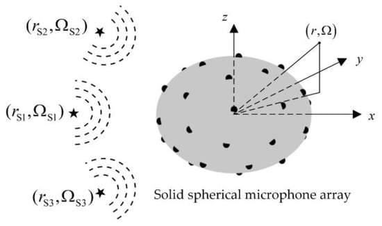
Figure 1.
Sound pressure signal model of a solid spherical array.
The sound pressure vector measured by the array can be written as
where is the sound pressure vector generated by the sound sources, is the independent stochastic noise, and is the propagation matrix from I sources to Q microphones. Here, SNR is defined as , where “” denotes the 2 norm. In , the element represents the sound pressure generated at the qth microphone by a unit intensity sound source located at the th source and is formulated as
where and denote spherical harmonics in the directions of and , respectively, both n and m are the degrees of spherical harmonics, the superscript “” denotes the conjugation, is the wavenumber corresponding to frequency f and the speed of sound c, and is the radial function. For spherical wave, is expressed as [7,8]
where and are the spherical Hankel function of the second kind and its derivative, respectively, and are the spherical Bessel function of the first kind and its derivative, respectively, and is the imaginary unit.
The measured sound pressure is further processed with FFT according to the Welch method [20], and the averaged CSM over multiple snapshots is obtained as follows
where “” is the expectation operator and the superscript “” represents the Hermitian transpose. The averaged CSM consists of the signal CSM
, the noise CSM , and additional crossed terms. Since noise signal is considered stochastic and independent of the source signals, the off-diagonal elements of and the crossed terms tend to zero as the number of snapshots tends to infinity. Therefore, the noise is mainly concentrated on the diagonal of C in the case of enough snapshots.
2.2. Reconstruction of the Measured CSM
Since FDAS requires the complete CSM C as input, its performance is affected by the noise on the diagonal of C, resulting in a significant degradation of acoustic imaging clarity in the presence of strong noise interference. In this subsection, the noise on the diagonal of C is removed by reconstructing the measured CSM with DRec, RPCA, and PFA, thus promoting the anti-noise interference capability of FDAS.
2.2.1. DRec
As explained previously, with a sufficient number of snapshots engaged in the averaging, the noise is mainly concentrated on the diagonal of C. The idea of DRec is to remove the noise auto-spectrum from the diagonal of C as much as possible, i.e., minimizing the sum of auto-spectrum in C while maintaining the denoised CSM positive semidefinite. Therefore, a diagonal matrix with unknown non-positive diagonal elements dq is added to C to cancel the noise auto-spectrum. The unknown diagonal elements dq are arranged in the vector , and then the solution problem of DRec can be formulated as [17]
where represents a diagonal matrix whose diagonal entries are the elements in vector , and the symbol “” represents positive semidefinite for a matrix. Equation (5) can be quickly solved using the CVX toolbox in MATLAB, and thus the denoised CSM can be estimated as
2.2.2. RPCA
RPCA utilizes the low-rankness of the signal CSM and the sparsity of the noise CSM to denoise the measured CSM. The rank of the signal CSM is determined by the number of incoherent sources. Considering that the number of incoherent main sources to be identified is usually smaller than the number of microphones, the signal CSM can be assumed to have low rank. Additionally, the noise CSM can be considered as a sparse diagonal matrix since the off-diagonal elements of the noise CSM tend to zero after multiple averaging. RPCA aims at recovering the low-rank signal matrix from noise-contaminated measurements, and its optimization problem can be expressed as [18]
where “” and “” denote the nuclear norm (sum of the eigenvalues) and the 1 norm respectively, “” stands for converting a matrix into a vector, and λ is the regularization parameter. Wright et al. [21] recommended and employed an accelerated proximal gradient algorithm to solve the above optimization problem, resulting in the denoised CSM being estimated as . In our case, with Q = 36, λ = 0.167 is adopted.
2.2.3. PFA
PFA is a probabilistic framework-based inference method, whose goal is to fit the measurements with the following model
where is the serial number of snapshots, is the source intensity vector of equivalent sound sources, and is a mixing matrix. is defined as the CSM of . The number of equivalent sound sources cannot be less than the number of true sound sources; otherwise, it is difficult to describe the sound field comprehensively. Since PFA still takes advantage of the fact that the noise is mainly concentrated on the diagonal of CSM after multiple averaging, the measured CSM is further modeled as follows:
In Equation (9), except that the measured CSM C is known, L, , and n are considered as random variables. The prior probability density functions (PDFs) assigned to the unknown variables are illustrated in Table 1.

Table 1.
Prior PDFs assigned to the unknown variables of PFA.
and denote the complex Gaussian PDF and the inverse gamma PDF (pair of conjugate distribution), respectively, and are the variance of equivalent sources and noise, and are two identity matrices with different dimensions, and the remaining hyperparameters ( and ) are constant [19].
In order to solve the fitting problem in Equation (9), the maximum a posteriori estimate of each unknown variable is established as follows [18]
where “” denotes conditional PDF. Here, the Gibbs sampler [22], a Markov Chain Monte Carlo algorithm, is used to find the above estimate, and then the denoised CSM can be expressed as
2.3. The Output of EFDAS
The output of EFDAS is constructed based on the denoised CSM . First, the eigenvalue decomposition of the denoised CSM is performed.
where is a diagonal matrix, are the eigenvalues of and satisfy , is an unitary matrix with the column being the eigenvector that corresponds to . Subsequently, the exponential function of is constructed as follows
where ξ is an exponent parameter. According to the literature [11], when ξ = 16, FDAS has strong sidelobe suppression and high quantization accuracy. In view of this, ξ = 16 is also recommended in EFDAS. Finally, the average pressure contribution of the focus point (rf, Ωf) [11], the arithmetic average of the microphone auto-spectrum generated by the source located at the focus point (rf, Ωf), is taken as the output of EFDAS.
where is the focus column vector of the focus point (rf, Ωf). In , the element represents the sound pressure generated at the th microphone by a unit intensity sound source located at the focus point (rf, Ωf), and it is defined as
Equations (2) and (15) are similar, but are used for forward sound field simulation and inverse focus of beamforming, respectively, which both require degree truncation of spherical harmonics [23], i.e., in Equation (2) and in Equation (15). In this case, EFDAS satisfies the high accuracy of sound source identification while maintaining a low computational cost.
3. Simulations
The simulations are carried out with a 36-channel solid spherical microphone array with a radius of 0.0975 m, as shown in Figure 1, which is also used in the subsequent experiment. The simulation steps are as follows: (1) Establish the array model and set the frequencies, intensities, and locations of the incoherent monopole sound sources to be identified. (2) Calculate the theoretical sound pressure emitted by the sound sources, add the noise n according to the SNR setting, and then obtain the total measured pressure and the corresponding CSM C. (3) Reconstruct the measured CSM C with DRec, RPCA, and PFA to acquire the denoised CSM . (4) Arrange the focus points on a spherical surface 1 m away from the array center with the spacing ∆θ = 5° and ∆φ = 5°, respectively, thus there creating a total of 37 × 72 focus points. (5) Calculate the EFDAS output of each focus point according to Equation (14), and thus perform the acoustic imaging.
3.1. Acoustic Imaging Colormaps
Acoustic imaging colormaps can intuitively reflect the localization and quantification of sound sources. In this subsection, acoustic imagings of FDAS and EFDAS are compared to demonstrate the performance enhancement of EFDAS. The maximum outputs of the mainlobes for true sources are labeled in the acoustic imaging maps, which are scaled to dB by referring to 2 × 10⁻⁵ Pa. Five sound sources with the coordinates (r, θ, φ) of (1 m, 90°, 180°), (1 m, 130°, 110°), (1 m, 50°, 110°), (1 m, 50°, 250°), and (1 m, 130°, 250°) are simulated, and their theoretical average sound pressure contributions are 94 dB, 91 dB, 88 dB, 85 dB, and 79 dB, respectively. Meanwhile, the display dynamic range of each map is set to 30 dB.
As shown in Figure 2, the ideal acoustic imaging colormaps of FDAS without noise interference are presented, with the columns from left to right corresponding to 1000 Hz, 3000 Hz, and 5000 Hz, in that order. It is clear that all sound sources are accurately located and quantified, which also proves the strong identification capability of FDAS for weak sources in the absence of noise interference.
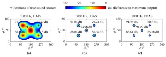
Figure 2.
Colormaps of FDAS without noise interference: (a) 1000 Hz; (b) 3000 Hz; (c) 5000 Hz.
Figure 3 shows the imaging colormaps of FDAS at SNR = 0 dB and discloses the influence of the number of snapshots. In Figure 3a–c, 10 snapshots are considered. Although there is no sidelobe contamination, the quantification errors of the sound sources are large, and multiple weak sources get lost. As shown in Figure 3d–f, the quantification errors markedly reduce when the number of snapshots increases to 100, but the imaging results suffer from severe sidelobe contamination. For the identification of weak sources, at 3000 Hz and 5000 Hz, since the amplitude of the weakest source is comparable to the sidelobes, the identification results are less reliable, and at 1000 Hz, there is no indication of the weakest source. The further increase in the number of snapshots fails to improve the imaging results, as illustrated in Figure 3g–i. The reasons why the number of snapshots has such an impact on the results of FDAS are that: (1) The measured CSM, which is the input of FDAS, requires a sufficient number of snapshots for averaging to correctly reflect the actual coherence between sound sources. (2) The insufficient number of snapshots causes part of the noise to remain on the off-diagonal elements of CSM. The residual noise power is equivalent to the sound sources and works with the true sources; hence, the actual output of FDAS deviates from the ideal output. As the number of snapshots increases, both the coherence between sound sources and the noise residual on the off-diagonal of CSM gradually decrease, allowing FDAS to locate and quantify sound sources with higher accuracy.
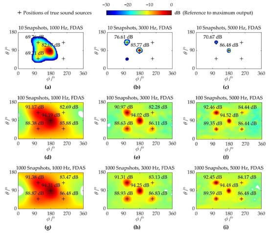
Figure 3.
Colormaps of FDAS with SNR = 0 dB and different snapshots: (a–c) Maps of FDAS with 10 snapshots at 1000 Hz, 3000 Hz, and 5000 Hz, respectively; (d–f) Maps of FDAS with 100 snapshots at 1000 Hz, 3000 Hz, and 5000 Hz, respectively; (g–i) Maps of FDAS with 1000 snapshots at 1000 Hz, 3000 Hz, and 5000 Hz, respectively.
Figure 4 shows the imaging colormaps of three EFDAS methods at SNR = 0 dB. The number of snapshots is set to 1000 (same with Figure 3g–i). In Figure 4, the columns from left to right are 1000 Hz, 3000 Hz, and 5000 Hz, and the rows from top to bottom correspond to EFDAS-DRec, EFDAS-RPCA, and EFDAS-PFA, respectively. Compared with Figure 3g–i, the sidelobes are much lower and the mainlobes are narrower in Figure 4a–c, which is attributed to the noise reduction with DRec. Moreover, all sources are identified at 3000 Hz and 5000 Hz, while at 1000 Hz, the weakest source gets lost and the mainlobes of strong sources are also seriously fused. Figure 4d–i shows that with the noise removal by RPCA and PFA, the sidelobes are eliminated in the display dynamic range, and the width of mainlobes is significantly decreased, allowing for clearer imaging and higher spatial resolution. Both EFDAS-RPCA and EFDAS-PFA can accurately locate all sources, and EFDAS-RPCA outperforms EFDAS-PFA in quantification accuracy for the weakest source (15 dB less than the strongest source).
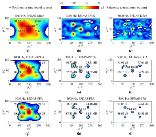
Figure 4.
Colormaps of EFDAS with SNR = 0 dB and 1000 snapshots: (a–c) Maps of EFDAS-DRec at 1000 Hz, 3000 Hz, and 5000 Hz, respectively; (d–f) Maps of EFDAS-RPCA at 1000 Hz, 3000 Hz, and 5000 Hz, respectively; (g–i) Maps of EFDAS-PFA at 1000 Hz, 3000 Hz, and 5000 Hz, respectively.
The acoustic imaging performance of EFDAS is summarized as follows: (1) EFDAS-RPCA and EFDAS-PFA can eliminate sidelobes in the display dynamic range, while EFDA-DRec still suffers from sidelobe contamination, despite a noticeable reduction in sidelobe amplitudes. (2) EFDAS-RPCA and EFDAS-PFA obviously improve spatial resolution by narrowing the mainlobes, while EFDAS-DRec only slightly enhances spatial resolution. (3) The three EFDAS methods enjoy a strong identification ability for weak sources, as they can accurately locate and quantify the sources that are 9 dB lower than the strongest source at SNR = 0 dB. Even for the sources that are 15 dB lower than the strongest source, the EFDAS methods are still able to locate them accurately, in spite of large quantification errors.
3.2. Performance Analysis
Furthermore, the effects of SNR and number of snapshots on CSM diagonal reconstruction error and the acoustic imaging accuracy are explored. The smaller diagonal reconstruction error of the signal CSM indicates the better noise reduction, and the higher acoustic imaging accuracy indicates the more accurate localization and quantification for sound sources. In this subsection, five sound sources of unequal intensity at 3000 Hz are adopted, which is consistent with those in Figure 2b.
3.2.1. Diagonal Reconstruction Error of Signal CSM
The relative error of diagonal elements between the denoised CSM and the noise-free CSM is defined as the diagonal reconstruction error .
where “” denotes the extraction of the diagonal elements of a matrix to construct a new vector.
The diagonal reconstruction errors of DRec, RPCA, and PFA are analyzed under different SNRs (from −10 to 10 dB with 2 dB steps) and different numbers of snapshots (100 × 2u, u = 0, 1, …, 7), respectively. Figure 5a shows the curves of δdiag vs. SNR when 1000 snapshots are considered, and Figure 5b shows the curves of δdiag vs. the number of snapshots at SNR = 0 dB. The curves for other combinations of SNR and the number of snapshots are similar to those in Figure 5. As can be seen in Figure 5, the diagonal reconstruction errors of DRec, RPCA, and PFA increase as SNR drops and decrease as the number of snapshots rises, indicating that more snapshots are required to maintain small diagonal reconstruction errors under lower SNRs. Moreover, the diagonal reconstruction errors of RPCA and PFA are comparable and much smaller than those of DRec, which is in general agreement with the findings in the literature [19].
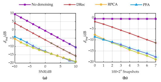
Figure 5.
Diagonal reconstruction errors under different SNRs and different numbers of snapshots: (a) different SNRs with 1000 snapshots; (b) different numbers of snapshots with SNR = 0 dB.
3.2.2. Acoustic Imaging Accuracy
The similarity between two vectors can be evaluated by the cosine of their angle. Therefore, define the similarity coefficient to describe the similarity between the vectorized actual and theoretical beamforming output.
where represents the actual beamforming output vector, represents the theoretical beamforming output vector with theoretical values at the true source positions and 0 at other positions, and the symbol “” denotes inner product operator. Define the difference coefficient as . The closer the difference coefficient is to 0, the more similar the beamforming output vector is to the theoretical output vector. When sources are accurately localized, the smaller difference coefficient reflects the fewer sidelobes and the narrower mainlobes, i.e., the better imaging clarity. Since the difference coefficient does not reflect quantification error, we further define the average quantification error η as
where and are the actual and the theoretical output in the direction of the ith sound source, respectively. When the difference coefficient ζ and the average quantification error η are close to zero, the actual beamforming output is close to the theoretical beamforming output. In that case, the actual acoustic imaging is close to the noise-free acoustic imaging, indicating the high acoustic imaging accuracy, i.e., great imaging clarity and accurate quantification.
Figure 6 shows the histograms of ζ and η vs. SNR and the number of snapshots, processed by FDAS, EFDAS-DRec, EFDAS-RPCA, and EFDAS-PFA, respectively. In general, as the number of snapshots and SNR increase, the difference coefficients and the average quantification errors of each EFDAS method gradually decrease, and the sound source identification performance gradually improves. Compared with FDAS, the difference coefficients of all EFDAS methods decrease. EFDAS-PFA has the smallest difference coefficient, followed by EFDAS-RPCA, and finally EFDAS-DRec, indicating that EFDAS-PFA has the strongest capability to suppress sidelobe contamination and reduce the width of mainlobe contamination, and thus enjoys the best imaging clarity. Moreover, EFDAS-DRec has the highest quantification accuracy and maintains a small quantification error even at SNR = −10 dB. EFDAS-RPCA and EFDAS-PFA show large quantification errors at the small number of snapshots and low SNRs. For the same SNR, EFDAS-PFA requires more snapshots to achieve quantification accuracy comparable to EFDAS-RPCA.
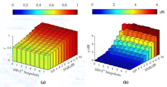
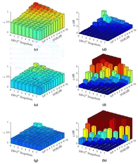
Figure 6.
Acoustic imaging errors: (a,c,e,g) The difference coefficients of FDAS, EFDAS-DRec, EFDAS-RPCA, and EFDAS-PFA, respectively; (b,d,f,h) The average quantification errors of FDAS, EFDAS-DRec, EFDAS-RPCA, and EFDAS-PFA, respectively.
3.3. Improvements of Acoustic Imaging Performance
Acoustic imaging accuracy describes the imaging quality in terms of both the difference coefficient and the average quantification error. Generally, the smaller the difference coefficient and the average quantification error, the better the imaging quality. However, the difference coefficient cannot separately describe the sidelobe suppression and the mainlobe shrinkage, and the average quantification error in Figure 6 cannot separately describe the quantification accuracy of strong and weak sources. Therefore, the maximum sidelobe level (MSL) is adopted to describe the amplitude of the sidelobes, and the number of grids in the mainlobe (NGM) within the 6 dB display dynamic range is defined to describe the size of mainlobe. additionally, the quantification and localization of weak sources are analyzed in this subsection.
3.3.1. Sidelobe Suppression and Mainlobe Reduction
MSL and NGM are simulated with a monopole source at different frequencies (from 1000 to 6000 Hz, with 500 Hz steps). A total of 20 Monte Carlo simulations are performed at each frequency, and in each simulation, the monopole source with an average sound pressure contribution of 94 dB is randomly arranged in a focus point. SNR = 0 dB and the number of snapshots of 1000 are set. Figure 7a shows the curves of MSL vs. frequency, which indicate that the MSL of EFDAS-PFA is the smallest at all frequencies, followed by EFDAS-RPCA, then EFDAS-DRec, and finally FDAS. Compared to FDAS, the average MSL of all frequencies is reduced by 6.4 dB for EFDAS-DRec, 21.6 dB for EFDAS-RPCA, and 53.1 dB for EFDAS-PFA. Figure 7b shows the curves of NGM vs. frequency, which indicate that the NGM of EFDAS-PFA is the smallest at all frequencies, followed by EFDAS-RPCA, then EFDAS-DRec, and finally FDAS. The shrinkage of the mainlobe for the three EFDAS methods is particularly noticeable at low frequencies. Compared to FDAS, the average NGM of all frequencies is reduced by 43.5% for EFDAS-DRec, 69.0% for EFDAS-RPCA, and 80.0% for EFDAS-PFA. Therefore, all three EFDAS methods can effectively suppress sidelobes and shrink the mainlobe, thus improving the imaging clarity. Among the three enhancement methods, EFDAS-PFA enjoys the best imaging clarity.
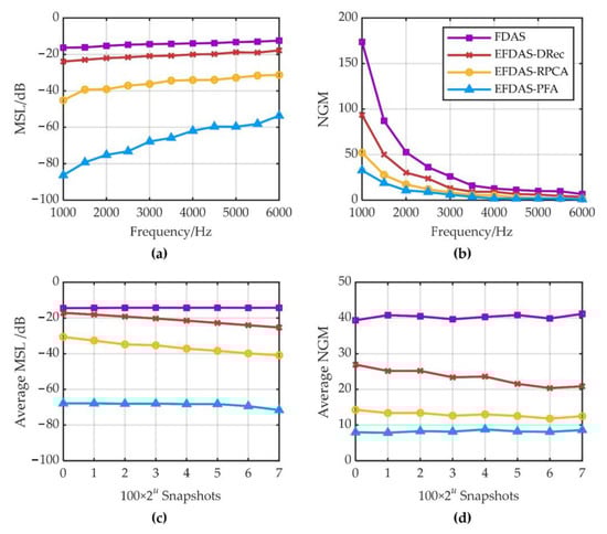
Figure 7.
MSL and NGM of FDAS and EFDAS at SNR = 0 dB: (a,b) MSL and NGM under different frequencies; (c,d) Average MSL and NGM under different numbers of snapshots.
The effects of the number of snapshots (100 × 2u, u = 0, 1,…,7) on MSL and NGM averaged over multiple frequencies (from 1000 to 6000 Hz, with 500 Hz steps) are further analyzed. Figure 7c,d shows the curves of the average MSL and the average NGM vs. the number of snapshots. It can be seen that the average MSL and average NGM of EFDAS-DRec and EFDAS-RPCA decrease with the increase in the number of snapshots, while those of FDAS and EFDAS-PFA are basically stable. The simulation results show that when the number of snapshots continues to increase from 100, it still improves the imaging clarity of EFDAS-DRec and EFDAS-RPCA, but has little effect on that of FDAS and EFDAS-PFA.
3.3.2. Quantification and Localization of Weak Sources
The excellent ability to identify weak sources is one of the advantages of FDAS; however, it is affected by noise interference. Although EFDAS is able to suppress noise by reconstructing the CSM, it leads to an underestimation of the intensity of the weak sources, which can be seen in Figure 4. In this subsection, the quantification and localization of weak sources are analyzed.
In Figure 8, five sound sources of varying intensity are simulated at SNR = 0 dB. The five sound sources are divided into two groups, one with the average sound pressure contribution of 94 dB, 91 dB, 88 dB, and 85 dB (strong sources), and the other with that of 79 dB (weak source). As shown in Figure 8, the average quantification errors η of the above two groups of sound sources vary with the number of snapshots. Figure 8 shows that: (1) The quantification errors of FDAS and EFDAS for the weak source are much larger than those for strong sources. (2) The average quantification errors of FDAS and EFDAS-DRec is less affected by the number of snapshots, and EFDAS-DRec consistently maintains a high quantification accuracy. (3) The quantification errors of EFDAS-RPCA and EFDAS-PFA decreases as the number of snapshots increases, reaching a quantification accuracy comparable to that of EFDAS-Rec, when the number of snapshots is 800~1600. Combining the diagonal reconstruction errors in Figure 5 and the average quantification errors in Figure 8, it is clear that EFDAS-RPCA and EFDAS-PFA are prone to decrease the quantification accuracy of weak sources, while significantly removing the noise.
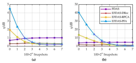
Figure 8.
Average quantification error under different numbers of snapshots: (a) Relatively strong sound sources (<−10 dB); (b) Weak source (−15 dB).
Although EFDAS-RPCA and EFDAS-PFA are prone to large quantification errors of weak sources, they are still able to locate weak sources effectively, due to the strong sidelobe suppression. Moreover, the quantification errors can be reduced by increasing the number of snapshots. To verify the excellent weak source localization capability of EFDAS, five sound sources with the average sound pressure contribution of 94 dB, 82 dB, 79 dB, 76 dB, and 73 dB are simulated. The coordinates of the sound sources are the same as with those in Figure 4. The imaging colormaps of the above sound sources at SNR = 0 dB are shown in Figure 9, where the number of snapshots is 1000 and the dynamic display range is 60 dB. As shown in Figure 9, all three EFDAS methods have enhanced the localization capability of weak sources for FDAS. Among the three EFDAS methods, EFDAS-PFA have the greatest weak source localization capability, followed by EFDAS-RPCA, and finally, EFDAS-DRec.
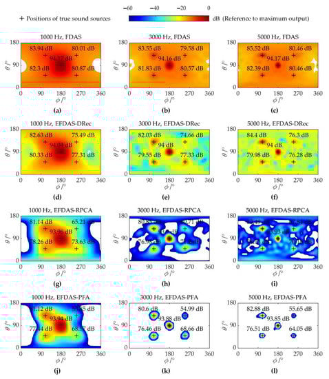
Figure 9.
Colormaps of FDAS and EFDAS with SNR = 0 dB and 1000 snapshots: (a–c) Maps of FDAS at 1000 Hz, 3000 Hz, and 5000 Hz, respectively; (d–f) Maps of EFDAS-DRec at 1000 Hz, 3000 Hz, and 5000 Hz, respectively; (g–i) Maps of EFDAS-RPCA at 1000 Hz, 3000 Hz, and 5000 Hz, respectively; (j–l) Maps of EFDAS-PFA at 1000 Hz, 3000 Hz, and 5000 Hz, respectively.
EFDAS-DRec, EFDAS-RPCA, and EFDAS-PFA all improve the sound source identification performance of FDAS under low SNRs, and the comparison among the performances of the three methods are summarized in Table 2. EFDAS-DRec has the weakest anti-noise interference capability and still cannot suppress sidelobes within the 30 dB dynamic range, but it has the advantages of high quantification accuracy, no manual setting parameters, and high calculation efficiency. EFDAS-RPCA offers strong noise suppression, clear imaging, accurate localization for weak sources, small quantification errors with sufficient snapshots, and particularly high computational efficiency. However, it involves selecting an appropriate regularization parameter , which has been discussed in Reference 14. EFDAS-PFA has slightly lower quantification accuracy than EFDAS-PRCA, but enjoys better imaging clarity and stronger weak source localization ability. Additionally, the computational efficiency of EFDAS-PFA improves with the decrease in the number of equivalent sources (as explained in Equation (8)), which is always larger than the number of true sources. In practice, a reasonable can be set according to the number of main sound sources of interest.
Table 2.
The comparison among the performances of three EFDAS methods.
4. Experiment
As shown in Figure 10, the validation experiment is conducted to examine the effectiveness of the proposed methods and the correctness of the simulation conclusions. A 36-channel solid spherical array from Brüel & Kjær with a radius of 0.0975 m is used to collect the sound pressure signals, where the coordinates of the array microphones are the same as those used in the simulations.
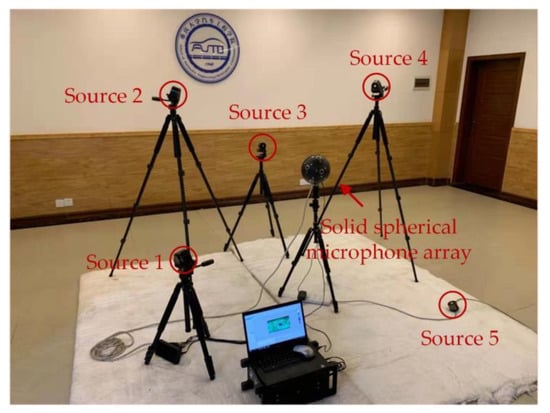
Figure 10.
Experimental layout.
Meanwhile, five loudspeaker sources with a radius of 0.025 m are arranged at different positions, and all are 1 m from the array center. During the experiment, each loudspeaker is independently excited by different steady-state Gaussian white noise, and the acoustic signals received by the array microphones are synchronously sampled by the PULSE Type 3660C data acquisition system at a sampling frequency of 16,384 Hz. The noise with SNR = 0 dB is artificially added to the measured time-domain sound pressure signal to simulate strong noise interference. In post-processing, we perform FFT on time-domain sound pressure signals to obtain the measured CSM averaged over multiple snapshots and apply different beamforming methods for acoustic imaging. A total of 500 snapshots participate in the FFT, with an overlap rate of 66.7%. Each snapshot is weighted with a Hanning window and has a length of 0.125 s, which corresponds to the frequency resolution of 8 Hz.
Figure 11 shows the experimental results. Each column from left to right corresponds to 1000 Hz, 3000 Hz, and 5000 Hz, and each row from top to bottom corresponds to FDAS, EFDAS-DRec, EFDAS-RPCA, and EFDAS-PFA. As shown in Figure 11a–c, the imaging results of FDAS suffer from severe sidelobe contamination, resulting in poor imaging clarity. Since the noise interference is even stronger than the weak sources, some of the sources are totally covered by sidelobes. Compared with FDAS, the imaging results of EFDAS-DRec in Figure 11d–f exhibit a noticeable decrease in the sidelobe magnitudes, resulting in improved imaging clarity at each frequency. Figure 11g–i illustrates the imaging results of EFDAS-RPCA, which reveal that the sidelobe contamination is largely eliminated in the dynamic range, the mainlobe width is significantly reduced, and all sources are accurately identified, except for the weakest source at 1000 Hz. In the imaging results of EFDAS-PFA, as shown in Figure 11j–m, the sidelobe contamination is completely eliminated, and the mainlobe width is further reduced. The above experimental findings are consistent with the simulation conclusions.
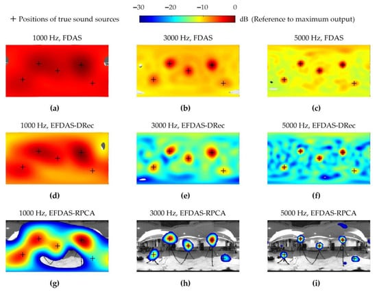
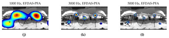
Figure 11.
Acoustic imaging colormaps of the experiment: (a–c) Maps of FDAS at 1000 Hz, 3000 Hz, and 5000, respectively; (d–f) Maps of EFDAS-DRec at 1000 Hz, 3000 Hz, and 5000, respectively; (g–i) Maps of EFDAS-RPCA at 1000 Hz, 3000 Hz, and 5000, respectively; (j–l) Maps of EFDAS-RPCA at 1000 Hz, 3000 Hz, and 5000 Hz, respectively.
5. Conclusions
To improve the sound source identification performance in low-SNR cabin environments, this paper introduces CSM reconstruction methods such as DRec, RPCA, and PFA, which are widely studied in planar arrays, into spherical arrays-based FDAS. Correspondingly, three enhancement methods, namely EFDAS-DRec, EFDAS-RPCA, and EFDAS-PFA, are established. The main conclusions obtained through simulations and experiments are as follows: (1) EFDAS can significantly improve the sound source identification performance of FDAS under low SNRs, that is, effectively suppress sidelobe contamination, shrink mainlobe contamination, and maintain the strong localization capability for weak sources. (2) Compared with FDAS at SNR = 0 dB and the number of snapshots = 1000, the average MSLs of EFDAS-DRec, EFDAS-RPCA, and EFDAS-PFA are reduced by 6.4 dB, 21.6 dB, and 53.1 dB, respectively, and the mainlobes of sound sources are shrunk by 43.5%, 69.0%, and 80.0%, respectively. (3) All three EFDAS methods can improve the quantification accuracy of FDAS when the number of snapshots is sufficiently large. EFDAS-DRec enjoys the best quantification accuracy and is less affected by the number of snapshots, while the quantification errors of EFDAS-RPCA and EFDAS-PFA are quite large with few snapshots, even worse than FDAS. (4) Among the three EFDAS methods, EFDAS-PFA has the strongest ability to localize weak sources, followed by EFDAS-RPCA, and finally, EFDAS-DRec.
Author Contributions
Conceptualization, Y.Z. and Z.C.; methodology, Y.Z.; software, Y.Z.; validation, Y.Z.; writing—original draft preparation, Y.Z.; writing—review and editing, Y.Z. and Z.C.; supervision, Y.Z., Z.C. and L.L. All authors have read and agreed to the published version of the manuscript.
Funding
This research was funded by the Science and Technology Project of China Southern Power Grid under Grant 036100KK52200034(GDKJXM20201968) and the National Natural Science Foundation of China under Grant 11774040.
Data Availability Statement
The data presented in this study are available on request from the corresponding author.
Conflicts of Interest
The authors declare no conflict of interest.
References
- Gil-Lopez, T.; Medina-Molina, M.; Verdu-Vazquez, A.; Martel-Rodriguez, B. Acoustic and economic analysis of the use of palm tree pruning waste in noise barriers to mitigate the environmental impact of motorways. Sci. Total Environ. 2017, 584, 1066–1076. [Google Scholar] [CrossRef] [PubMed]
- Amran, M.; Murali, G.; Khalid, N.H.A.; Fediuk, R.; Ozbakkaloglu, T.; Lee, Y.H.; Haruna, S.; Lee, Y.Y. Slag uses in making an ecofriendly and sustainable concrete: A review. Constr. Build. Mater. 2021, 272, 121942. [Google Scholar] [CrossRef]
- Chiariotti, P.; Martarelli, M.; Castellini, P. Acoustic beamforming for noise source localization—Reviews, methodology and applications. Mech. Syst. Signal Proc. 2019, 120, 422–448. [Google Scholar] [CrossRef]
- Sun, H.; Yan, S.; Svensson, U.P. Robust minimum sidelobe beamforming for spherical microphone arrays. IEEE Trans. Audio Speech Lang. Process. 2011, 19, 1045–1051. [Google Scholar] [CrossRef]
- Wang, D.; Guo, J.; Xiao, X.; Sheng, X. CSA-based acoustic beamforming for the contribution analysis of air-borne tyre noise. Mech. Syst. Signal Proc. 2022, 166, 108409. [Google Scholar] [CrossRef]
- Haddad, K.; Hald, J. 3D localization of acoustic sources with a spherical array. In Proceedings of the 7th European Conference on Noise Control 2008, EURONOISE 2008, Pairs, France, 29 June–4 July 2008; pp. 1585–1590. [Google Scholar]
- Hald, J. Spherical beamforming with enhanced dynamic range. SAE Int. J. Passeng. Cars Mech. Syst. 2013, 6, 1334–1341. [Google Scholar] [CrossRef]
- Chu, Z.; Yang, Y.; He, Y. Deconvolution for three-dimensional acoustic source identification based on spherical harmonics beamforming. J. Sound Vib. 2015, 344, 484–502. [Google Scholar] [CrossRef]
- Yang, Y.; Chu, Z.; Shen, L.; Ping, G.; Xu, Z. Fast fourier-based deconvolution for three-dimensional acoustic source identification with solid spherical arrays. Mech. Syst. Signal Proc. 2018, 107, 183–201. [Google Scholar] [CrossRef]
- Dougherty, R.P. Functional beamforming. In Proceedings of the 5th Berlin Beamforming Conference, Berlin, Germany, 19–20 February 2014. BeBeC-2014-S01. [Google Scholar]
- Yang, Y.; Chu, Z.; Shen, L.; Xu, Z. Functional delay and sum beamforming for three-dimensional acoustic source identification with solid spherical arrays. J. Sound Vib. 2016, 373, 340–359. [Google Scholar] [CrossRef]
- Chu, Z.; Zhao, S.; Yang, Y.; Yang, Y. Deconvolution using CLEAN-SC for acoustic source identification with spherical microphone arrays. J. Sound Vib. 2019, 440, 161–173. [Google Scholar] [CrossRef]
- Hald, J.; Kuroda, H.; Makihara, T.; Ishii, Y. Mapping of contributions from car-exterior aerodynamic sources to an in-cabin reference signal using Clean-SC. In Proceedings of the 45th International Congress and Exposition on Noise Control Engineering: Towards a Quieter Future, INTER-NOISE 2016, Hamburg, Germany, 21–24 August 2016; pp. 3732–3743. [Google Scholar]
- Dinsenmeyer, A.; Leclère, Q.; Antoni, J.; Julliard, E. Comparison of microphone array denoising techniques and application to flight test measurements. In Proceedings of the 25th AIAA/CEAS Aeroacoustics Conference, Delft, The Netherlands, 20–23 May 2019; pp. 2744–2753. [Google Scholar]
- Hald, J. Denoising of cross-spectral matrices using canonical coherence. J. Acoust. Soc. Am. 2019, 146, 399–408. [Google Scholar] [CrossRef] [PubMed]
- Dougherty, R.P. Cross spectral matrix diagonal optimization. In Proceedings of the 6th Berlin Beamforming Conference, Berlin, Germany, 29 February–1 March 2016. BeBeC-2016-S02. [Google Scholar]
- Hald, J. Removal of incoherent noise from an averaged cross-spectral matrix. J. Acoust. Soc. Am. 2017, 142, 846–854. [Google Scholar] [CrossRef] [PubMed]
- Dinsenmeyer, A.; Antoni, J.; Leclère, Q.; Pereira, A. On the denoising of cross-spectral matrices for (aero) acoustic applications. In Proceedings of the 7th Berlin Beamforming Conference, Berlin, Germany, 5–6 March 2018. BeBeC-2018-S02. [Google Scholar]
- Dinsenmeyer, A.; Antoni, J.; Leclère, Q.; Pereira, A. A probabilistic approach for cross-spectral matrix denoising: Bechmarking with some recent methods. J. Acoust. Soc. Am. 2020, 147, 3108–3123. [Google Scholar] [CrossRef] [PubMed]
- Jin, Z.; Han, Q.; Zhang, K.; Zhang, Y. An intelligent fault diagnosis method of rolling bearings based on Welch power spectrum transformation with radial basis function neural network. J. Vib. Control 2020, 26, 629–642. [Google Scholar] [CrossRef]
- Wright, J.; Peng, Y.; Ma, Y. Robust principal component analysis: Exact recovery of corrupted low-rank matrices by convex optimization. In Proceedings of the 23rd Annual Conference on Neural Information Processing Systems 2009, NIPS 2009, Vancouver, BC, Canada, 7–10 December 2009; pp. 2080–2088. [Google Scholar]
- Antoni, J.; Vanwynsberghe, C.; Magueresse, T.L.; Bouley, S.; Gilquin, L. Mapping uncertainties involved in sound source reconstruction with a cross-spectral-matrix-based Gibbs sampler. J. Acoust. Soc. Am. 2019, 146, 4947–4961. [Google Scholar] [CrossRef] [PubMed] [Green Version]
- Chu, Z.; Yang, Y.; Yang, Y. A new insight and improvement on deconvolution beamforming in spherical harmonics domain. Appl. Acoust. 2021, 177, 107900. [Google Scholar] [CrossRef]
Publisher’s Note: MDPI stays neutral with regard to jurisdictional claims in published maps and institutional affiliations. |
© 2022 by the authors. Licensee MDPI, Basel, Switzerland. This article is an open access article distributed under the terms and conditions of the Creative Commons Attribution (CC BY) license (https://creativecommons.org/licenses/by/4.0/).