A 3D Range-Only SLAM Algorithm Based on Improved Derivative UKF

Abstract

In this study, we constructed a 3D range-only (RO) localization algorithm based on improved unscented Kalman filtering (UKF). The algorithm can determine the location of unknown UWB nodes in a 3D environment through a moving node with low computational complexity, which can help agents to accurately identify feature points in 3D SLAM based only on the range. Specifically, we established an original UKF framework based the 3D RO localization algorithm, and developed a derivative UKF framework to reduce the computational complexity of the algorithm. We used singular value decomposition to compensate for the robustness of the algorithm. Next, we performed a theoretical analysis to show that our method reduces the computational burden without reducing the stability or accuracy of the system. Finally, we conducted numerical simulations and physical experiments to show the effectiveness of the developed 3D RO localization algorithm.

1. Introduction

Most of the current ultra-wideband (UWB) localization systems are implemented in indoor environments, for example, in tunnels, factories, warehouses, etc. [1], where UWB anchors are deployed beforehand and multiple nodes can be localized using their distance to the anchors. This localization scheme cannot be used for localization in the absence of UWB anchors (or in an unknown environment). The range-only localization approach can be used to deal with this problem, which uses only the distance measurements via UWB modules [2]. The study of localization without the assistance of UWB anchors has important theoretical and practical value for exploring unknown indoor environments and underground passages.

Unlike other traditional SLAM methods [3], RO-SLAM only needs to use the distance measurements between the robot and the feature points for robot localization and mapping [4]. As its main principle, RO-SLAM adopts the range-only localization algorithm to estimate the location of feature points and construct SLAM maps composed of the location information of the feature points. The sensors applied in the current mainstream RO-SLAM methods include Bluetooth, WiFi, RFID, UWB, etc. In practical applications, Bluetooth modules are equipped on many smart devices and provide advantages in device deployment [5]. However, Bluetooth modules have poor anti-interference performance and limited coverage. The insufficient localization accuracy of WiFi devices does not meet actual engineering requirements [6,7], and the short effective working distance of RFID technology has limited its applications [8]. Compared to these technologies, UWB systems can provide centimeter-level positioning accuracy in the absence of obstacle occlusion. UWB also has a strong penetration ability, low power consumption, high transmission rate, and a variety of technical advantages, which had led to UWB technology being widely used in industry [9].

The RO-SLAM framework has been intensively studied [10,11]. Recently, underwater node points and unmanned boats were located using only long baseline hydroacoustic devices [12]. Menegatti et al [13] introduced RO-localization into a SLAM system consisting of an unmanned vehicle and a wireless sensor network, where the positions of sensor nodes were back-projected from multiple positions of the unmanned vehicle. Bluetooth sensors can be applied to determine the range between unmanned vehicles; on this basis, an RO-SLAM framework was developed for interconnected robotic communication and cooperative multirobot localization [14,15]. A region-based particle filter [16] based on the RO-SLAM algorithm was proposed reduce the number of particles and improve real-time performance, which was verified on an unmanned vehicle platform equipped with UWB sensors [17]. Torres-González and colleagues proposed a scalable distributed RO-SLAM scheme that uses robot-node collaboration to provide real-time performance while improving SLAM accuracy. This algorithm was integrated in an unmanned aerial system (UAS) and evaluated in a 3D SLAM outdoor experiment [18,19].

Although many solutions have been proposed for the localization problem in RO-SLAM, many results were achieved by adopting the original EKF and UKF to estimate the node positions. The original EKF method is widely used in RO-SLAM to locate feature points; however, the accuracy of the system decreases when faced with high nonlinearity and cannot meet application requirements [20,21]. The original UKF-based RO-localization methods do not have many limitations in terms of nonlinear strength, but their computational complexity is too high, which has limited their development [22,23].

To deal with the above-mentioned problems, in this study:

• We constructed a 3D range-only localization algorithm to solve both the localization problem for uncalibrated UWB nodes in an indoor environment and the feature point localization problem in 3D RO-SLAM.
• Considering the time-invariant property of the state evolution equation, we constructed a derivative RO-SLAM algorithm to improve the real-time performance of the positioning system. Moreover, we introduced the SVD decomposition method to improve the robustness of the system.
• We verified the effectiveness of the proposed algorithm through simulation examples as well as practical experiments on UAV platforms.

In summary, we propose a UWB-system-based 3D RO-localization algorithm to achieve the localization of uncalibrated UWB nodes in 3D RO-SLAM. Considering the real-time and robustness requirements of the system, we further improved the algorithm and applied it to a UAV platform.

The rest of the paper is organized as follows: In Section 2, the system dynamics and observation models are established. By analyzing the shortcomings of the current RO-localization method, an overall improvement scheme is proposed. Next, an unscented Kalman filter based 3D RO-localization algorithm is proposed in Section 3 to achieve the localization of UWBs, which is called derivative unscented Kalman filter (DUKF). The DUKF uses the KF to simplify the computation of measurement updates without degrading the estimation accuracy. Furthermore, SVD decomposition is applied to the DUKF algorithm to ensure the stability of the algorithm. In Section 4, the computational complexity and stability of the proposed algorithm are theoretically analyzed. In Section 5, the feasibility of the algorithm is verified through simulation and UVA platform experiments. Finally, conclusions are drawn in Section 6.

The terminologies associated with the filtering algorithms in this paper are explained in

Table 1. Definition of filtering algorithm abbreviations used in this paper.

Abbreviation	Explanation
KF	A method for state estimation of linear systems.
UKF	A method for state estimation of nonlinear systems.
DUKF	A derivative algorithm is proposed by combining the KF and UKF algorithms. The KF and UKF algorithms are used for the linear and nonlinear parts of the system, respectively.
SVD-DUKF	The Cholesky decomposition for calculating sigma points in the DUKF algorithm is replaced with SVD decomposition.

.

The relationship between the filtering algorithms used in this study is illustrated in Figure 1.

2. System Modeling and Problem Formulation

2.1. System Model

In this study, we considered a UAV system equipped with UWB and IMU sensors. To localize uncalibrated UWB nodes in an indoor 3D environment using a UAV, the position of the UAV and the UWB range information need to be measured. An IMU can quickly provide accurate position and orientation information of the UAV; however, accelerometer errors in the IMU may lead to drift-error accumulation over time. Although the UWB cannot provide complete attitude information, its positioning results are relatively stable and its positioning accuracy does not change over time. In this study, the UAV relied on the IMU to provide motion information, combined with the UWB ranging information, to localize UWB nodes and predictively correct the UAV motion trajectory. We combined the UAV motion model and UWB sensors to build an RO-localization system model.

Figure 2 shows that, differently from the traditional multistation localization algorithm, the range-only localization algorithm uses the distance measurements of the moving UAV at different times. The detailed theoretical derivation of this algorithm is provided in Section 3. The dynamic measurement model is described below.

The UAV position measurement is based on IMU and UWB sensors. Here, we chose the position of the UWB node as the state quantity and the velocity information of the IMU as the system input. The UWB modules considered in this study are spatially distributed, where all nodes and anchors are treated as UWB nodes without any distinction. Assuming that the indoor environment is an ideal three-dimensional environment, the location of the UAV-carried No. 0 UWB node is denoted as $p_0={\left[\begin{array}{c}{x}_0,y_0,z_0\hfill \end{array}\right]}^T$ and the velocity is $v_0={\left[\begin{array}{c}{v}_{0,x},v_{0,y},v_{0,z}\hfill \end{array}\right]}^T$. The No. n uncalibrated UWB node position in a 3D environment is denoted as ${\left[\begin{array}{c}{x}_n,y_n,z_n\hfill \end{array}\right]}^T,n=1,2,\dots ,N$, where N is the number of UWB nodes. The state vector of the system is defined as:

$$X_k={\left[\begin{array}{c}{p}_{0,k},p_{1,k},\dots ,p_{N,k}\hfill \end{array}\right]}^T$$

(1)

which represents the locations of all UWB nodes at time k. By incorporating the IMU characteristics, the state-space system of the RO-SLAM model is:

$$X_{k+1}=A{X}_k+B{u}_k+w_k$$

(2)

where the state transfer matrix $A=I_{3N+3}$, the input matrix $B={\left[T\times I_3,0_{3\times 3N}\right]}^T$, and T is the sampling period. The input vector is the velocity information provided by the IMU $u_k=v_{0,k}$, and the process noise $w_k$ is Gaussian white noise with its variance $Q_k$ expressed as:

$$E\left[w_k{w}_k^T\right]=Q_k$$

(3)

The measurement equations are obtained based on UWB ranging information. We assume that there are $N+1$ UWB nodes in the system, the UAV carries the No. 0 node, and other unknown UWB nodes are randomly distributed in the 3D environment. All UWB nodes are available for ranging between themselves and the UAV. The ranging information at time k between the No. i node and the UAV can be expressed as the Euclidean distance, as follows:

$$d_{i,k}=\sqrt{{\left(x_{i,k}-x_{0,k}\right)}^2+{\left(y_{i,k}-y_{0,k}\right)}^2+{\left(z_{i,k}-z_{0,k}\right)}^2}$$

(4)

where $i=0,1,\dots ,N$. The measurement equation can be expressed as:

$$Z_k=\left[\begin{array}{c}{d}_{0,1,k}\\ ⋮\\ d_{0,i,k}\end{array}\right]+v_k$$

(5)

where the measurement noise $v_k$ is Gaussian white noise, with its variance $R_k$ being expressed by:

$$E\left[v_k{v}_k^T\right]=R_k$$

(6)

2.2. Problem Formulation

Given the system model (1)–(6), in the localization problem considered in this study, the state sequence $X_k$ is estimated using the distance measurements $Z_k$, where the state vector $X_k$ consists of the time-varying positions of the UAV and the static positions of the rest of the UWB nodes. The developed localization approach can algorithmically be applied to the calibration of UWB anchors without any manual effort. UWB sensors are characterized by an ability to provide centimeter-level ranging accuracy between nodes, and the problem of reverse calculating the location of UWB nodes in space by the distance between nodes can be achieved using only the RO-localization algorithm.

However, as introduced in the Section 1, the existing RO-localization algotithms are generally adopt the EKF for state estimation. Although EKF technology is mature and EKF has a small calculation burden, its accuracy is unsatisfactory, especially in 3D environments where the nonlinearity of the system is higher.

In this study, we made the following efforts to improve the traditional RO-localization algorithm:

• Improve the localization accuracy of the 3D RO-localization algorithm;
• Reduce the computational complexity of the 3D RO-localization algorithm;
• Verify the performance of the algorithm on a physical platform.

To improve the localization accuracy, we first considered adopting the UKF instead of the EKF in RO-localization. To reduce the computational complexity, given the characteristics of the linear state evolution equation and the nonlinear measurement equation, we adopted the derivative method [24] to reduce the redundant calculations in the linear part to reduce the computational complexity of the state update. Finally, we built a physical platform to verify the performance of the proposed algorithm in an actual environment. In addition, we used SVD decomposition to replace the Cholesky decomposition to improve the stability of the filtering algorithm [25].

3. 3D Range-Only Localization Algorithm

3.1. Algorithm Overview

RO-SLAM is a special SLAM method that relies on ranging sensors to localize the feature points in a map. The mechanism of the RO-localization algorithm is visually illustrated in Figure 3: when the UAV is not moving, relying on a single range value can only be used to infer the possible position of the unknown node on a circle. As the UAV moves along the x-axis direction, the uncertainty in the x-axis direction gradually decreases, but the y-axis direction still has large uncertainty. As the UAV moves along the y-axis, the uncertainty in the y-axis direction is reduced and the position of the unknown node eventually converges to an acceptable range. These features of RO-SLAM have led to its wide use in sensor calibration and search and rescue.

To solve the inverse localization problem of unknown UWB nodes in a 3D environment using the distance measurements of the UAV, we adopted the RO-localization framework. The observation model of the system in Section 2.1 is a nonlinear model. To improve the localization accuracy and avoid large truncation errors, similar to those experienced with EKF, we established a UKF framework to solve the RO-localization problem.

The UKF uses UT transform to achieve linear approximation based on the mean and variance approximation, which was first proposed by Julier et al. [26]. In this study, they proved that the accuracy of the UT transform is not lower than the linear approximation based on the third-order Taylor expansion, and the existing EKF is usually based on the first- or second-order Taylor expansion. This leads to the estimation accuracy of the UKF being higher than that of the EKF. Therefore, we developed a UKF-based RO-localization algorithm to improve the estimation accuracy of inversion localization.

However, since UT transform needs to obtain sigma points and their state prediction multiple times, the computational complexity of the UKF is much higher than that of the first-order Taylor-expansion-based EKF. To cope with this problem, we further developed a derivative algorithm based on the UKF based RO-localization algorithm to reduce the computational complexity.

3.2. Reduction in Computational Complexity

The linear Kalman filter (KF) cannot be used for calculation because the observation model of the system is nonlinear (as described in Section 2.1). Accordingly, we introduced the unscented Kalman filter (UKF), which helps achieve accurate results. However, $2n+1$ sigma points must be implemented with the complete filtering processes in the UKF during the linearization of the nonlinear model. This substantially increases the complexity of the calculation.

We noticed that the system has a linear state model, as shown in Equation (2), and a nonlinear observation model, as shown in Equation (4). Hu et al. [24] proposed a derivative method to reduce the computational complexity of the system where either the system state model or the system observation model is linear. In other words, the standard KF is used for processing the linear part of the system, while the mean- and variance-based linear approximation is applied for the nonlinear part. In our previous work [27], we employed the same idea to successfully reduce the computational complexity of UWB-based location systems. Here, we also introduced derivative methods to reduce the computational burden. The specific steps of the algorithm are as follows:

First, the system state prediction can be directly updated in linear time for the given initial value of the iteration (${\widehat{X}}_k$) and the initial error covariance ($P_k$), because the system has a linear state equation, as shown in Equation (2).

$${\widehat{X}}_{k+1\mid k}=A{\widehat{X}}_k+w_k$$

(7)

$$P_{k+1|k}=A{P}_k{A}^T+Q_k$$

(8)

Then, the Sigma point set can be calculated based on Equations (7) and (8):

$$\left\{\begin{array}{c}{\eta }_{k+1}^0={\widehat{X}}_{k+1\mid k}\hfill \\ {\eta }_{k+1}^i={\widehat{X}}_{k+1\mid k}+S_{k+1\mid k}\sqrt{(n+\lambda )},(1\le i\le n)\hfill \\ {\eta }_{k+1}^i={\widehat{X}}_{k+1\mid k}-S_{k+1\mid k}\sqrt{(n+\lambda )},(n+1\le i\le 2n)\hfill \end{array}\right.$$

(9)

where $\lambda$ is the scaling parameter, which controls the sampling interval of the sigma point around $x_{k+1|k}$; n is the dimension of the system state vector, which was 15 in this study; $S_{k+1|k}$ is obtained by Cholesky decomposition of the error covariance $P_{k+1|k}$. Then, the measurement of the obtained sigma points can be predicted:

$${\zeta }_{k+1}^i=H\left({\eta }_{k+1}^i\right),(0\le i\le 2n)$$

(10)

where ${\zeta }_{k+1}^i$ represents the measurement prediction of the ith sigma point at time $k+1$. Then, we can calculate the measurement prediction and covariance of the system at time $k+1$:

$${\widehat{Z}}_{k+1\mid k}=\sum _{i=0}^{2n}{\omega }_m^i{\zeta }_{k+1}^i$$

(11)

$$P_{{\widehat{Z}}_{k+1\mid k}}=\sum _{i=0}^{2n}{\omega }_c^i\left({\zeta }_{k+1}^i-{\widehat{Z}}_{k+1\mid k}\right){\left({\zeta }_{k+1}^i-{\widehat{Z}}_{k+1\mid k}\right)}^T+R_k$$

(12)

where $\omega$ is the weight of the ith sigma point, which is usually determined by the following equation:

$$\left\{\begin{array}{c}{\omega }_m^0=\frac{\lambda }{n+\lambda }\hfill \\ {\omega }_c^0=\frac{\lambda }{n+\lambda }+\left(1-{\alpha }^2+\beta \right)\hfill \\ {\omega }_m^i={\omega }_c^i=\frac{\lambda }{2(n+\lambda )},(1\le i\le 2n)\hfill \end{array}\right.$$

(13)

Subsequently, we can calculate the cross-covariance between the system state prediction and the measurement prediction based on the state prediction of the system, the sigma point set, and the associated measurement prediction at time $k+1$:

$$P_{{\widehat{X}}_{k+1}{\widehat{Z}}_{k+1}}=\sum _{i=0}^{2n}{w}_c^i\left({\eta }_{k+1}^i-{\widehat{X}}_{k+1\mid k}\right){\left({\zeta }_{k+1}^i-{\widehat{Z}}_{k+1\mid k}\right)}^T$$

(14)

Then, the Kalman gain K can be obtained:

$$K_{k+1}=P_{{\widehat{X}}_{k+1}{\widehat{Z}}_{k+1}}{P}_{{\widehat{Z}}_{k+1\mid k}}^{-1}$$

(15)

Finally, the system state and covariance can be updated based on the Kalman gain K:

$${\widehat{X}}_{k+1}={\widehat{X}}_{k+1\mid k}+K_{k+1}\left(Z_{k+1}-{\widehat{Z}}_{k+1\mid k}\right)$$

(16)

$$P_{k+1}=P_{k+1|k}-K_{k+1}{P}_{{\widehat{Z}}_{k+1\mid k}}{K}_{k+1}^T$$

(17)

As is shown in Equations (7) and (8), many redundant calculations of sigma points are avoided due to the application of linear update in the state prediction stage, which considerably reduces the overall computational burden of the algorithm. A specific quantitative analysis of the computational complexity is provided in Section 4.1.

3.3. Robustness

The introduction of the derivative algorithm successfully lowers the overall computational complexity by eliminating redundant calculations in the state prediction part. However, during the experiments, we found that the estimation error covariance matrix is often positive semidefinite, which causes the filtering process to be unstable.

The reason for this problem is that the Cholesky decomposition adopted in the UKF and DUKF requires the decomposed matrix to be strictly positive. To deal with this problem, singular value decomposition (SVD) was proposed to replace Cholesky decomposition in the UKF [25], which can more effectively decompose the positive semidefinite covariance matrix and improve the robustness of the algorithm. Similarly, we also introduced SVD into the DUKF algorithm in this study. The specific steps of the improved algorithm are as follows:

As shown in Equation (9), $S_{k+1|k}$ is calculated by decomposing the error covariance $P_{k+1|k}$ using the Cholesky decomposition. In comparison, here, we use the SVD method to decompose $P_{k+1|k}$. When $P_{k+1|k}$ is a non-negative definite symmetric matrix, we have:

$$P_{k+1|k}=U_{k+1|k}{\Lambda }_{k+1|k}{U_{k+1|k}}^T$$

(18)

With ${\Lambda }_{k+1|k}={D_{k+1|k}}^2$, we have:

$$P_{k+1|k}=U_{k+1|k}{D}_{k+1|k}{D}_{k+1|k}{U}_{k+1|k}^T$$

(19)

Substituting Equation (19) into Equation (9) yields:

$$\left\{\begin{array}{c}{\eta }_{k+1}^0={\widehat{x}}_{k+1\mid k}\hfill \\ {\eta }_{k+1}^i={\widehat{x}}_{k+1\mid k}+U_{k+1|k}{D}_{k+1|k}\sqrt{(n+\lambda )},(1\le i\le n)\hfill \\ {\eta }_{k+1}^i={\widehat{x}}_{k+1\mid k}-U_{k+1|k}{D}_{k+1|k}\sqrt{(n+\lambda )},(n+1\le i\le 2n)\hfill \end{array}\right.$$

(20)

Then, we can use the sigma points obtained in Equation (20) to replace Equation (9). This operation is the essence of the SVD-DUKF algorithm. The specific steps of the SVD-DUKF-based 3D RO-SLAM algorithm are provided below.

3.4. Detailed Steps of the Algorithm

After integrating SVD-DUKF into the 3D range-only RO-SLAM proposed in Section 3.2, we obtained a simplified algorithm that can complete similar tasks but has a lower computational burden, which we call the SVD-DUKF-based 3D Range-only RO-SLAM algorithm. The specific steps of this algorithm are shown in Algorithm 1.

Algorithm 1: Detailed steps of the range-only 3D RO-SLAM based on SVD-DUKF.

Input:${\widehat{X}}_k$, $P_k$, $u_k$

Output:${\widehat{X}}_{k+1}$, $P_{k+1}$, $A1$–$A4$

1. Perform linear state prediction on $P_k$ and ${\widehat{X}}_k$ to obtain $P_{k+1|k}$ and ${\widehat{X}}_{k+1\mid k}$;

2. Implement SVD on $P_{k+1|k}$ to obtain $D_{k+1|k}$;

3. Calculate the sigma point according to Equation (20) to obtain $\begin{array}{cc}{\eta }_{k+1}^i,& i=0,\dots ,2n\end{array}$;

4. Calculate the measurement prediction of the sigma point according to the measurement equation, and obtain $\begin{array}{cc}{\zeta }_{k+1}^i,& i=0,\dots ,2n\end{array}$;

5. Combine the sigma points to obtain the overall measurement prediction of the system ${\widehat{Z}}_{k+1\mid k}$;

6. Calculate the measurement covariance $P_{{\widehat{Z}}_{k+1\mid k}}$ based on the measurement prediction of the system and sigma points;

7. Calculate system cross-covariance $P_{{\widehat{X}}_{k+1}{\widehat{Z}}_{k+1}}$ based on measurement prediction and state prediction;

8. Calculate the Kalman gain K based on the measured covariance $P_{{\widehat{Z}}_{k+1\mid k}}$ and cross-covariance $P_{{\widehat{X}}_{k+1}{\widehat{Z}}_{k+1}}$;

9. Update the system state and error covariance to obtain $P_{k+1}$ and ${\widehat{X}}_{k+1}$;

10. Strip the 4th to 12th elements in $A1$–$A4$ as $A1$–$A4$ and output them as the results of the RO-SLAM algorithm;

11. Set $P_{k+1}$ and ${\widehat{X}}_{k+1}$ as the new initial values, and repeat steps 1–10.

12. end.

4. Analysis of Computational Complexity and Stability

In the previous section, we improved the estimation accuracy and computational complexity of the original 3D RO-localization algorithm, and ensured its robustness. In this section, we analyze the computational complexity and stability of the proposed algorithm.

4.1. Computational Complexity Analysis

In this study, each multiplication or addition operation was defined as a flop. The total number of flops represented the computational complexity of the algorithm.

Table 2. Computational complexity analysis of three systems.

Step	Algorithm	Original System (5 + 5)	Augmented System (6 + 6)	Simplified Augment System (6 + 4)
Calculation of Cubature Points	$\begin{array}{c}{P}_k=S_k{S}_k^{-1}\hfill \\ {\xi }_{j,k}=S_k{\chi }_j+X_k\hfill \\ {\xi }_{j,k+1|k}=A\left({\xi }_{j,k}\right)\hfill \end{array}$	450 flops	792 flops	508 flops
		460 flops	844 flops	538 flops
		200 flops	552 flops	300 flops
Time update	$X_{k+1|k}={\displaystyle \sum _{j=1}^m}{\omega }_j{\xi }_{j,k+1|k}$	50 flops	72 flops	52 flops
Prediction of covariance update	$\begin{array}{c}{P}_{k+1|k}={\displaystyle \sum _{j=1}^m}{\omega }_j(X_{k+1|k}-{\xi }_{j,k+1|k})·\hfill \\ {(X_{k+1|k}-{\xi }_{j,k+1|k})}^T+Q_k\hfill \end{array}$	260 flops	372 flops	270 flops
Measurement forecast	$Z_{k+1|k}=H\left(X_{k+1|k}\right)$	90 flops	132 flops	94 flops
Calculation of Kalman gain	$\begin{array}{c}{K}_k=P_{k+1|k}{H}^T·{(H{P}_{k+1|k}{H}^T+R_k)}^{-1}\hfill \end{array}$	1504 flops	2596 flops	1684 flops
Status update	$X_{k+1}=X_{k+1|k}+K_k(Z_{k+1}-Z_{k+1|k})$	30 flops	36 flops	30 flops
Covariance update	$P_{k+1}=(I-P_{k+1|k}H)P_{k+1|k}$	950 flops	1656 flops	1068 flops
Total	N/A	3994 flops	7052 flops	4544 flops

shows the computational complexity of the original UKF and SVD-DUKF algorithms with 15-dimensional state equations and 10-dimensional observation equations for the system described in Section 2.1.

As shown in Table 2, the simplified SVD-DUKF algorithm requires 3054 flops (43.42%) less than the original UKF algorithm in each iteration. Therefore, we concluded that the simplified SVD-DUKF algorithm successfully reduces the computational burden of the RO-SLAM algorithm in the filtering process. The simulation results supporting this conclusion are provided in Section 5.2.

4.2. Stability Analysis

The stability analysis and lower bounds of error for DUKF were provided by Hu et al. [28]. They proved that the DUKF has similar stability to and lower bounds of error than the original UKF. However, although they proved that the DUKF can achieve convergence under positive semidefinite error covariance, the Cholesky decomposition cannot be applied to semipositive semidefinite matrices. Therefore, the filter cannot continue to run when the covariance matrix is positive semidefinite. They added a minimal positive definite matrix to the error covariance matrix during each iteration to ensure the matrix is positive definite as the solution. However, the added matrix affects the estimation accuracy of the filter after multiple iterations. Especially in the case of high sensor accuracy or long-term estimation, this situation becomes more serious. For this problem, we introduced SVD decomposition to the DUKF. The final result is that the proposed SVD-DUKF algorithm has similar stability to and error lower bounds than the original UKF, and can operate under positive semidefinite error covariance matrices.

5. Experiment Verification

To verify the performance of the algorithms proposed in Section 3 and Section 4, we conducted numerical simulations on an x86 microcomputer and physical experiments on a UAV platform. Next, we introduce the simulation settings and the experimental details.

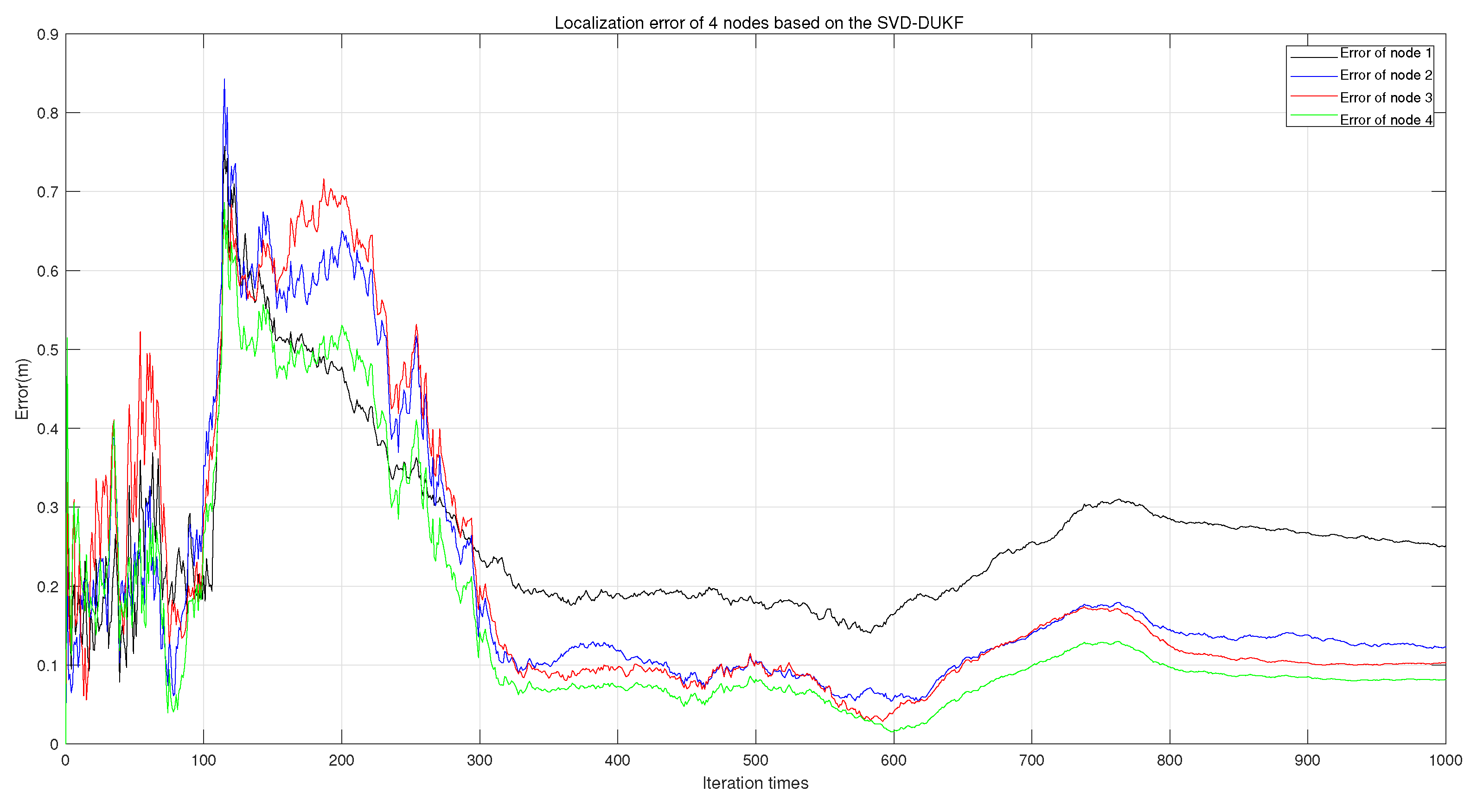
5.1. Numerical Simulations

To verify the performance of the proposed algorithms, we simulated the UKF- and SVD-DUKF-based algorithms on an x86 PC with an Intel Core i5 7500 CPU with 16 GB memory. The simulation environment was MATLAB 2019a. The system models adopted in the numerical simulation were described in Section 2.1. We added uncorrelated Gaussian noise as the process noise of the system, and the measurement noise conformed to a normal distribution. In the simulations, we tested the original UKF-based and SVD-DUKF-based RO localization algorithms, and we simulated a total of 1500 Monte Carlo experiments and took the mean of their results to evaluate their localization accuracy and computational burden. Because the UKF is no less accurate than the EKF with linearized approximation by third-order Taylor expansion [26], the EKF, in practice, is usually based on linearized approximation by first-order Taylor expansion. Therefore, the accuracy of the EKF is theoretically much lower than that of the UKF. For this reason, we only performed numerical simulations of original UKF- and SVD-DUKF-based algorithms in this study. The specific parameters of simulation are shown in

Table 3. Parameters used in the simulation.

Item	Parameter
Initial state	UAV coordinate: $x_1={[1,1,0]}^T$
	Controls : Changes with time
	node 1 coordinate: $A1={[9,5,6]}^T$
	node 2 coordinate: $A2={[8,12,3]}^T$
	node 3 coordinate: $A3={[3,8,6]}^T$
	node 4 coordinate: $A4={[6,10,4]}^T$
	$X_1={[x_1,A1,A2,A3,A4]}^T$
Simulation time	1000 (/s)
Sampling time	$T=1$
Initial estimate $X_1$	${\widehat{X}}_1=X_1+N\left(\begin{array}{cc}0,& P_1\end{array}\right)$
Initial covariance $P_1$	15-order diagonal identity matrix
Driving function of process noise	$\begin{array}{c}G=\left[\begin{array}{ccc}{w}_u& \cdots & 0_{\times 12}\\ ⋮& \ddots & ⋮\\ 0_{\times 12}& \cdots & 0_{\times 12}\end{array}\right]\hfill \\ w_u=\left[\begin{array}{ccc}T& 0& 0\\ 0& T& 0\\ 0& 0& T\end{array}\right]\hfill \end{array}$
Distribution of process noise $w_k$	$N(0,0.09)$
Distribution of measurement noise $r_k$	$N(0,0.05)$

.

The simulation results are shown in Figure 4, Figure 5 and Figure 6. Figure 4 shows the average localization error of each node from 1500 Monte Carlo trials. The figure shows that the two algorithms have similar error curves for the localization of all four nodes, which shows that the two algorithms have basically consistent localization performance. Figure 5 and Figure 6 show samples of the two filtering algorithms with 1500 Monte Carlo trials, where these two algorithms show similar performance.

Table 4. Average calculation time.

Item	Original UKF-Based Algorithm	SVD-DUKF-Based Algorithm
Average Calculation time (s)	0.5376	0.4826

shows the average calculation time required for the 1500 Monte Carlo trials for the two algorithms. The calculation time of the SVD-DUKF based algorithm is about 10.24% lower compared to that of the original UKF-based algorithm. In the theoretical analysis in Section 4.1, the calculation complexity of the simplified algorithm was reduced by more than 20% due to the calculation of the other parts of the entire algorithm except filtering, such as SVD decomposition.

According to the simulation results, the simplified RO-SLAM algorithm proposed in Section 4 has similar precision to the original algorithm but a computational burden that is lower by about 10%. This allows the UAVs to use a lower-energy CPU to obtain a longer airborne time or a higher system refresh rate to achieve compliant control.

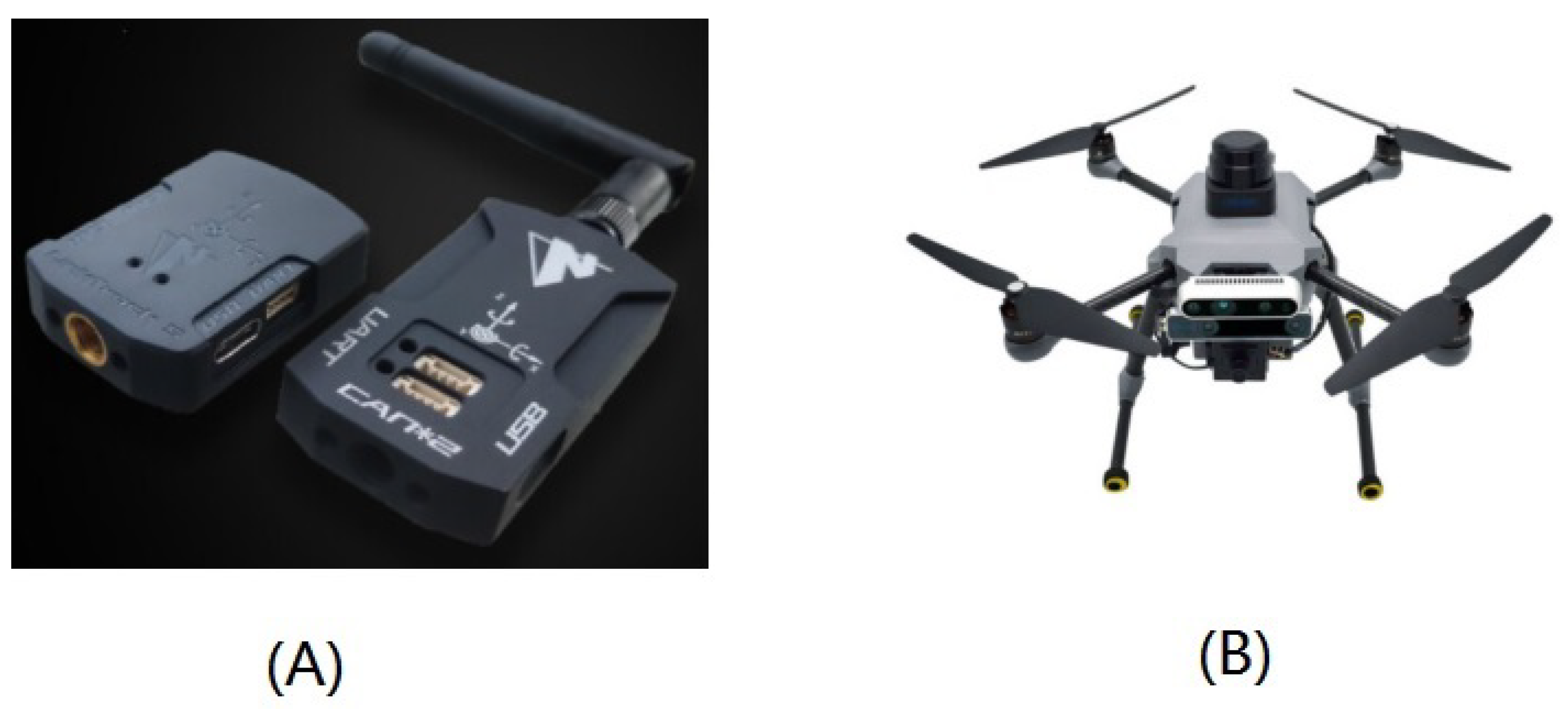
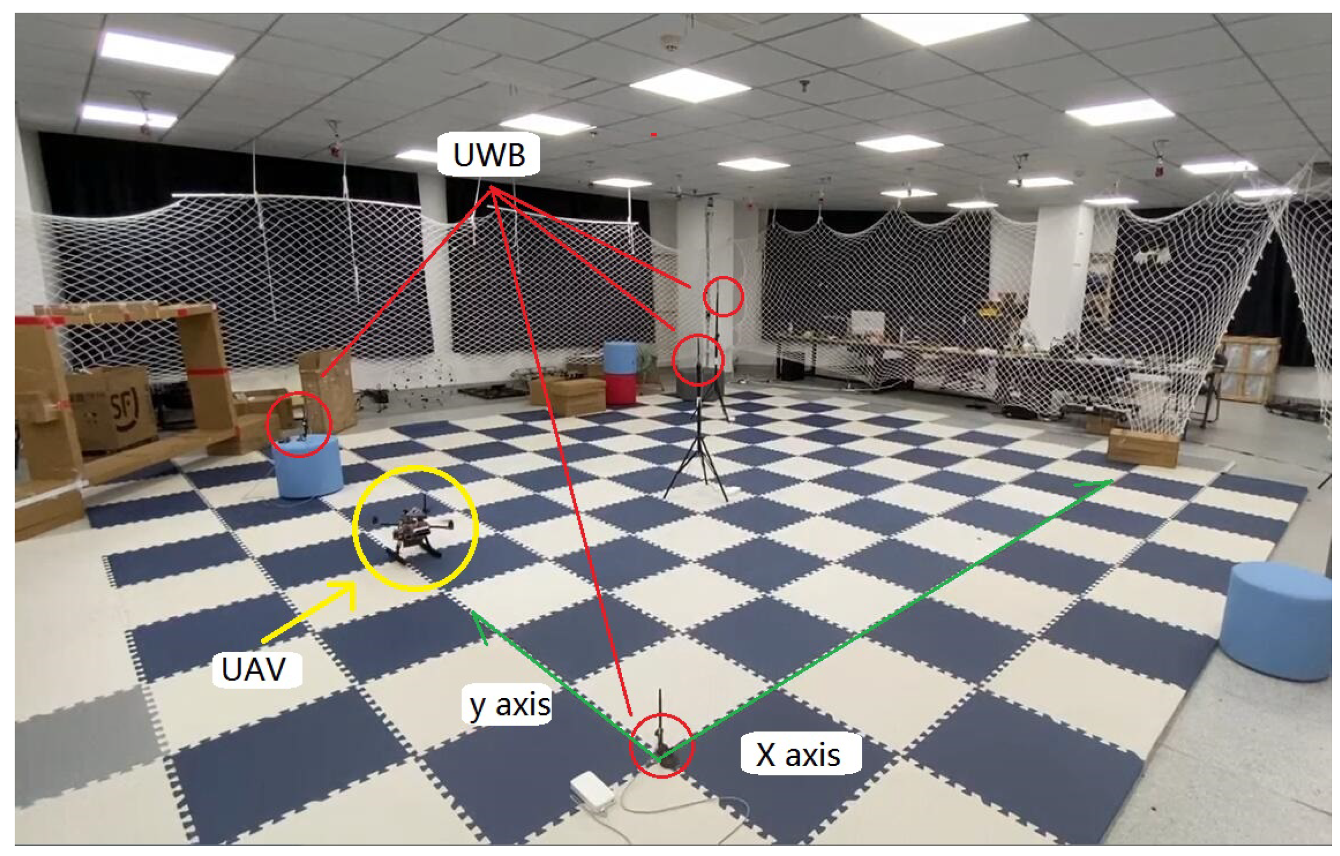
5.2. Physical Experiment

After verifying the performance of the proposed algorithm through numerical simulations, we used the data of a physical UAV to verify the actual performance of the proposed algorithm. The hardware adopted in the experiment is shown in Figure 7, and the specific technical parameters are provided in

Table 5. Hardware parameters.

Item	Details
Onboard CPU	Nvidia Jetson Xavier NX
Hashrate	21TOPs
Flight control system	Pixhawk
Onboard OS	Promeheus V1.0
Size	335 × 335 × 230 mm
Rotor number	4
Diagonal wheelbase	410 mm
Ranging accuracy	2D: mean 10 cm, standard deviation 5 cm
	3D: mean 30 cm, standard deviation 15 cm
Maximum range	500 m
Maximum frequency	200 Hz

. The actual states of each node is obtained by manual measurement.

The experimental scene is shown in Figure 8. We placed four UWB nodes with different heights in the experimental site. Each UWB node had complete ranging and communication functions, and the fifth UWB node (also had complete functions) was equipped on the UAV. The position of node 1 was the origin of the x-axis and y-axis, and the ground altitude of the UAV was the origin of the z-axis. We had the UAV take off and fly back to the starting point, we recorded the data obtained by the UWB sensors during this flight, and performed RO-localization. The video of the experiment can be found at [https://www.bilibili.com/video/BV1Tr4y1k7rU/ (accessed on 22 March 2022)]. The parameters set in the experiment are provided in

Table 6. Parameters used in the experiment.

Parameter	Values
Initial state	UAV coordinate: $x_1={[0,0,0.24]}^T$
	Controls: Changes with time
	node 1 coordinate: $A1={[2.023,0,1.06]}^T$
	node 2 coordinate: $A2={[0,2.023,0.52]}^T$
	node 3 coordinate: $A3={[4.046,2.023,1.5]}^T$
	node 4 coordinate: $A4={[0,-2.023,0.14]}^T$
	$X_1={[x_1,A1,A2,A3,A4]}^T$
Simulation time	69 (/s)
Sampling time	$T=0.05$
Initial estimate $X_1$	15 × 1 Identity matrix vector
Initial covariance $P_1$	15-order diagonal identity matrix
Distribution of process noise $w_k$	$N(0,0.0081)$
Distribution of measurement noise $r_k$	$N(0,0.022)$

(some parameters that were the same as in the simulation are not described in detail, and can be found in Table 3).

The results are shown in Figure 9: the final convergence error of the physical experiment is similar to that of the result of the simulation. Therefore, the SVD-DUKF-based 3D range-only localization algorithm proposed in this paper can be applied for precise localization of fixed nodes in a 3D environment with range-only measurements.

However, node 2 had a high localization error that showed a tendency to increase. After analyzing the data of the UWB rangefinder, we found that the ranging information of the node 2 had some non-Gaussian noise. As a result, the RO-localization position information of node 2 was considerably affected. In addition, as shown in Figure 10, this noise was proportional to the magnitude of the range values and showed a Gaussian distribution when the range values were similar. Based on this characteristic, we think that this occurred due to the longer distance between node 2 and the UAV, which caused flicker noise during range measurement. In future research, we will attempt to solve this problem.

6. Conclusions

In this paper, we proposed the SVD-DUKF-based RO-localization algorithm for locating unknown UWB nodes in a 3D environment based only on distance measurements of a moving UWB module. By exploiting the linear property of the state evolution equation, the algorithm was improved by reducing the computational burden while ensuring localization accuracy. In addition, to solve the convergence problem caused by linearization approximation error, singular value decomposition was incorporated into the derivative algorithm. Through simulation examples and practical experiments, we showed that the proposed method can provide accurate 3D localization of uncalibrated UWB nodes in an indoor environment. This allows the UAV to more precisely locate feature points in a map in 3D based on range-only measurement, which enables better completion of the 3D RO-SLAM task.

The following aspects will be investigated in our future work:

1

The effect of non-Gaussian noise in the positioning process.

2

Integrating the proposed algorithm into a 3D RO-SLAM program for experiments to verify its practical performance in SLAM tasks.

3

Extending the 3D RO-SLAM algorithm to dynamic environments for development in cooperative UAV localization.

References

1. Li, Z.; Wang, R.; Gao, J.; Wang, J. An Approach to Improve the Positioning Performance of GPS/INS/UWB Integrated System with Two-Step Filter. Remote Sens. 2017, 10, 19. [Google Scholar] [CrossRef] [Green Version]
2. Djugash, J.; Singh, S.; Kantor, G.; Wei, Z. Range-only SLAM for robots operating cooperatively with sensor networks. In Proceedings of the 2006 IEEE International Conference on Robotics and Automation, Orlando, FL, USA, 15–19 May 2006. [Google Scholar]
3. Khairuddin, A.R.; Talib, M.S.; Haron, H. Review on simultaneous localization and mapping (SLAM). In Proceedings of the 2015 IEEE International Conference on Control System, Computing and Engineering (ICCSCE), Penang, Malaysia, 27–29 November 2015; pp. 85–90. [Google Scholar]
4. Blanco, J.L.; Fernandez-Madrigal, J.A.; Gonzalez, J. Efficient probabilistic Range-Only SLAM. In Proceedings of the IEEE/RSJ International Conference on Intelligent Robots & Systems, St. Louis, MO, USA, 10–15 October 2008. [Google Scholar]
5. Kajioka, S.; Mori, T.; Uchiya, T.; Takumi, I.; Matsuo, H. Experiment of indoor position presumption based on RSSI of Bluetooth LE beacon. In Proceedings of the 2014 IEEE 3rd Global Conference on Consumer Electronics (GCCE), Tokyo, Japan, 7–10 October 2014. [Google Scholar]
6. Fei, W.; Li, Y.; Hua, J. WiFi Location System Based on Position Fingerprint Algorithm. Microcontroll. Embed. Syst. 2014, 2014, 29–32. [Google Scholar]
7. Nass, M. Wi-Fi Based Range-Only Constraint Integration in RTAB-Map. Master’s Thesis, University of Twente, Enschede, The Netherlands, 2020. [Google Scholar]
8. Montaser, A.; Moselhi, O. RFID indoor location identification for construction projects. Autom. Constr. 2014, 39, 167–179. [Google Scholar] [CrossRef]
9. García, E.; Poudereux, P.; Hernández, Á.; Ureña, J.; Gualda, D. A robust UWB indoor positioning system for highly complex environments. In Proceedings of the 2015 IEEE International Conference on Industrial Technology (ICIT), Seville, Spain, 17–19 March 2015; pp. 3386–3391. [Google Scholar]
10. Haykin, S. Kalman Filtering and Neural Networks; John Wiley & Sons: Hoboken, NJ, USA, 2004; Volume 47. [Google Scholar]
11. Kehagias, A.; Djugash, J.; Singh, S. Range-Only Slam with Interpolated Range Data; Robotics Institute: Pittsburgh, PA, USA, 2006. [Google Scholar]
12. Chen, W.; Sun, R. Range-Only SLAM for Underwater Navigation System with Uncertain Beacons. In Proceedings of the 2018 10th International Conference on Modelling, Identification and Control (ICMIC), Guiyang, China, 2–4 July 2018; pp. 1–5. [Google Scholar]
13. Menegatti, E.; Zanella, A.; Zilli, S.; Zorzi, F.; Pagello, E. Range-only slam with a mobile robot and a wireless sensor networks. In Proceedings of the 2009 IEEE International Conference on Robotics and Automation, Kobe, Japan, 12–17 May 2009; pp. 8–14. [Google Scholar]
14. Lim, H.; Myung, H. Effective Indoor Robot Localization by Stacked Bidirectional LSTM Using Beacon-Based Range Measurements. In Proceedings of the International Conference on Robot Intelligence Technology and Applications, Kuala Lumpur, Malaysia, 16–18 December 2018; pp. 144–151. [Google Scholar]
15. Soria, P.R.; Palomino, A.F.; Arrue, B.; Ollero, A. Bluetooth network for micro-uavs for communication network and embedded range only localization. In Proceedings of the 2017 International Conference on Unmanned Aircraft Systems (ICUAS), Miami, FL, USA, 13–16 June 2017; pp. 747–752. [Google Scholar]
16. Gustafsson, F. Particle filter theory and practice with positioning applications. IEEE Aerosp. Electron. Syst. Mag. 2010, 25, 53–82. [Google Scholar] [CrossRef] [Green Version]
17. Wang, J.; Meng, Z.; Wang, L. Efficient Probabilistic Approach to Range-Only SLAM With a Novel Likelihood Model. IEEE Trans. Instrum. Meas. 2021, 70, 1–12. [Google Scholar] [CrossRef]
18. Torres-González, A.; Martínez-de Dios, J.R.; Ollero, A. Robot-beacon distributed range-only SLAM for resource-constrained operation. Sensors 2017, 17, 903. [Google Scholar] [CrossRef] [PubMed] [Green Version]
19. Torres-González, A.; Martinez-de Dios, J.R.; Ollero, A. Range-only SLAM for robot-sensor network cooperation. Auton. Robot. 2018, 42, 649–663. [Google Scholar] [CrossRef]
20. Lee, H.; Chun, J.; Jeon, K.; Lee, H. Efficient ekf-slam algorithm based on measurement clustering and real data simulations. In Proceedings of the 2018 IEEE 88th Vehicular Technology Conference (VTC-Fall), Chicago, IL, USA, 27–30 August 2018; pp. 1–5. [Google Scholar]
21. Sato, A.; Nakajima, M.; Kohtake, N. Rapid BLE beacon localization with range-only EKF-SLAM using beacon interval constraint. In Proceedings of the 2019 International Conference on Indoor Positioning and Indoor Navigation (IPIN), Pisa, Italy, 30 September–3 October 2019; pp. 1–8. [Google Scholar]
22. Zhang, Q.; Niu, B.; Zhang, W.; Li, Y. Feature-based ukf-slam using imaging sonar in underwater structured environment. In Proceedings of the 2018 IEEE 8th International Conference on Underwater System Technology: Theory and Applications (USYS), Wuhan, China, 1–3 December 2018; pp. 1–5. [Google Scholar]
23. Ammann, N.; Mayo, L.G. Undelayed initialization of inverse depth parameterized landmarks in UKF-SLAM with error state formulation. In Proceedings of the 2018 IEEE/ASME International Conference on Advanced Intelligent Mechatronics (AIM), Auckland, New Zealand, 9–12 July 2018; pp. 918–923. [Google Scholar]
24. Hu, G.; Gao, S.; Zhong, Y. A derivative UKF for tightly coupled INS/GPS integrated navigation. ISA Trans. 2015, 56, 135–144. [Google Scholar] [CrossRef] [PubMed]
25. Hoecker, A.; Kartvelishvili, V. SVD approach to data unfolding. Nucl. Instrum. Meth. A 1996, 372, 469–481. [Google Scholar] [CrossRef] [Green Version]
26. Julier, S.; Uhlmann, J.; Durrant-Whyte, H.F. A new method for the nonlinear transformation of means and covariances in filters and estimators. IEEE Trans. Autom. Control 2000, 45, 477–483. [Google Scholar] [CrossRef] [Green Version]
27. Tang, C.; Dou, L. An Improved Game Theory-Based Cooperative Localization Algorithm for Eliminating the Conflicting Information of Multi-Sensors. Sensors 2020, 20, 5579. [Google Scholar] [CrossRef] [PubMed]
28. Gaoge, H. Extension Research on UKF Algorithm and Data Fusion Technology for Integrated Navigation; NPU: Xi’an, China, 2016. [Google Scholar]
Figure 1. Relationship between filtering algorithms.
Electronics 11 01109 g001
Figure 2. RO-SLAM schematic diagram. The blue dotted line represents the flight path of the UAV over a period of time, the blue dots represent the position of the UAV at different times, and the blue triangle is the node to be located.
Electronics 11 01109 g002
Figure 3. Possible positions of an uncalibrated node as the UAV moves. (a) The initial position of the UAV and uncalibrated node; (b) the possible positions of the uncalibrated nodes at the initial moment; (c) as the UAV moves along the x-axis direction, the uncertainty in the x-axis direction gradually decreases; (d) as the UAV moves along the y-axis direction, the uncertainty in the y-axis direction gradually decreases.
Electronics 11 01109 g003
Figure 4. Average localization errors of 4 nodes in 1500 Monte Carlo trials. The red line represents the RO localization based on the original UKF, and the blue line represents the RO localization based on SVD-DUKF.
Electronics 11 01109 g004
Figure 5. One Monte Carlo trial of the UKF-based 3D RO-localization algorithm.
Electronics 11 01109 g005
Figure 6. One Monte Carlo trial of the SVD-DUKF-based 3D RO-localization algorithm.
Electronics 11 01109 g006
Figure 7. Sensor and UAV adopted in this study: (A) LinkTrack-P UWB rangefinder (NoopLoop, Shenzhen, China); (B) P450 UAV (Amovlab, Chengdu, China).
Electronics 11 01109 g007
Figure 8. Experiment scene.
Electronics 11 01109 g008
Figure 9. Localization error of UWB nodes in a physical experiment.
Electronics 11 01109 g009
Figure 10. Range measurement of node 2.
Electronics 11 01109 g010