
Practical Nonlinear Model Predictive Controller Design for Trajectory Tracking of Unmanned Vehicles


Abstract
:1. Introduction
- (1)
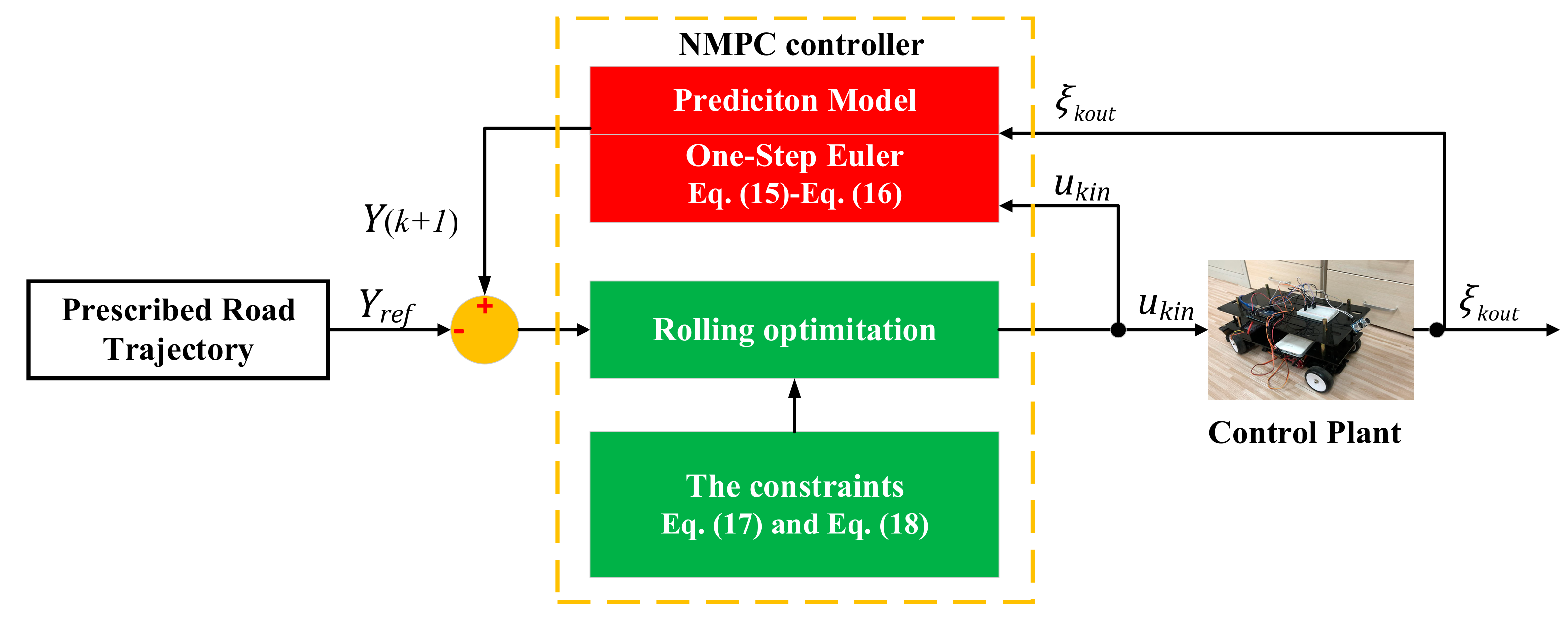
- A novel NMPC controller is proposed to achieve the accurate trajectory tracking of the UV under different prescribed roads, wherein the one-step Euler method is used to establish the nonlinear prediction model. As model predictive control is an iterative process, the Euler method has the advantages of a wide range of numerical solutions, a simple form that is easy to calculate, thus the tracking errors of forward velocity and yaw angle are minimized through a nonlinear optimization method;
- (2)
- MATLAB simulations are carried out to verify the control performances of the proposed NMPC controller under two different driving scenarios, and the results show that the strategy can deal with the nonlinear road trajectory well, and can improve the tracking accuracy and the driving stability;
- (3)
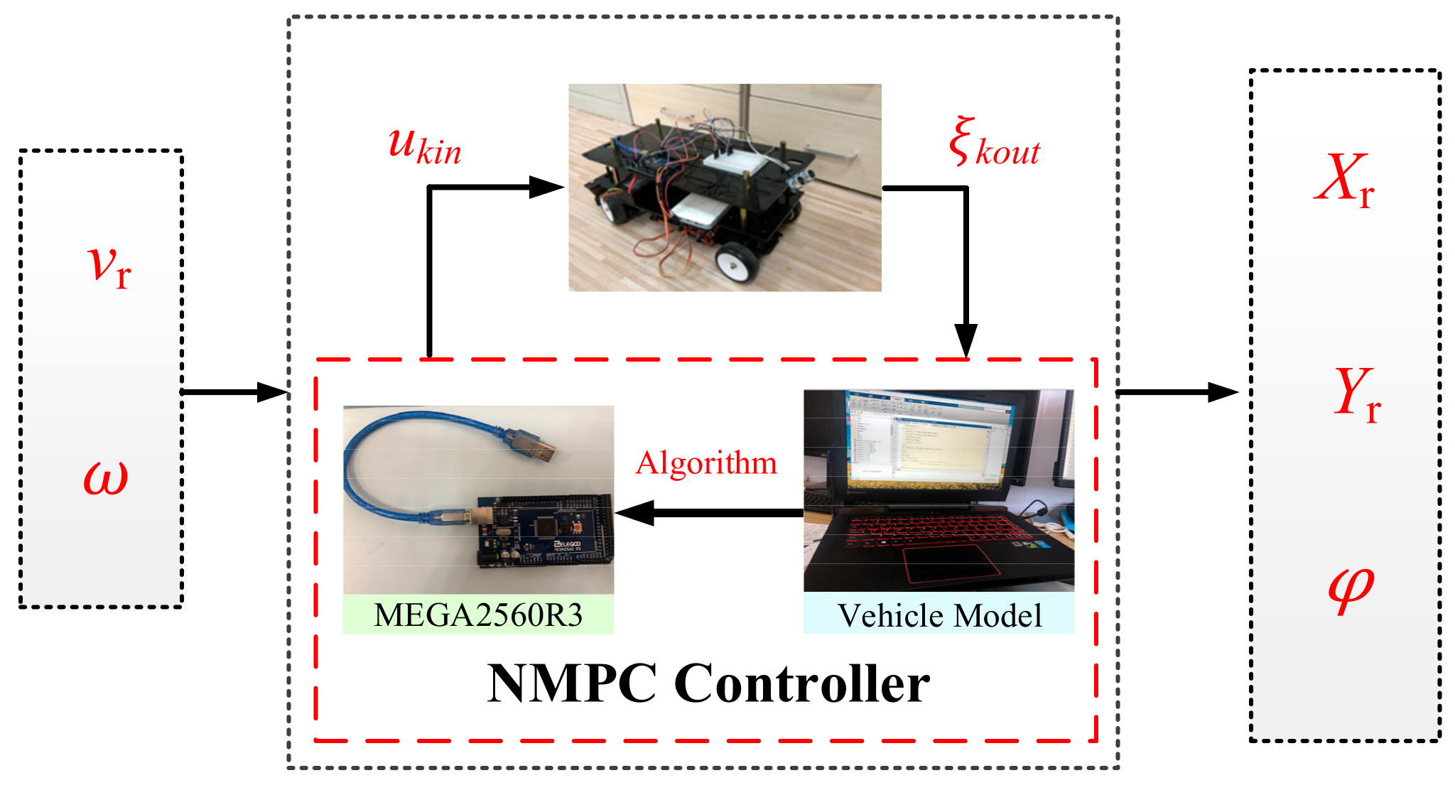
- A simple test platform consisting of a scaled-down real racing car, sensors, microcontroller, and host computer is built up to verify the effectiveness of the designed NMPC controller in UV trajectory tracking applications.
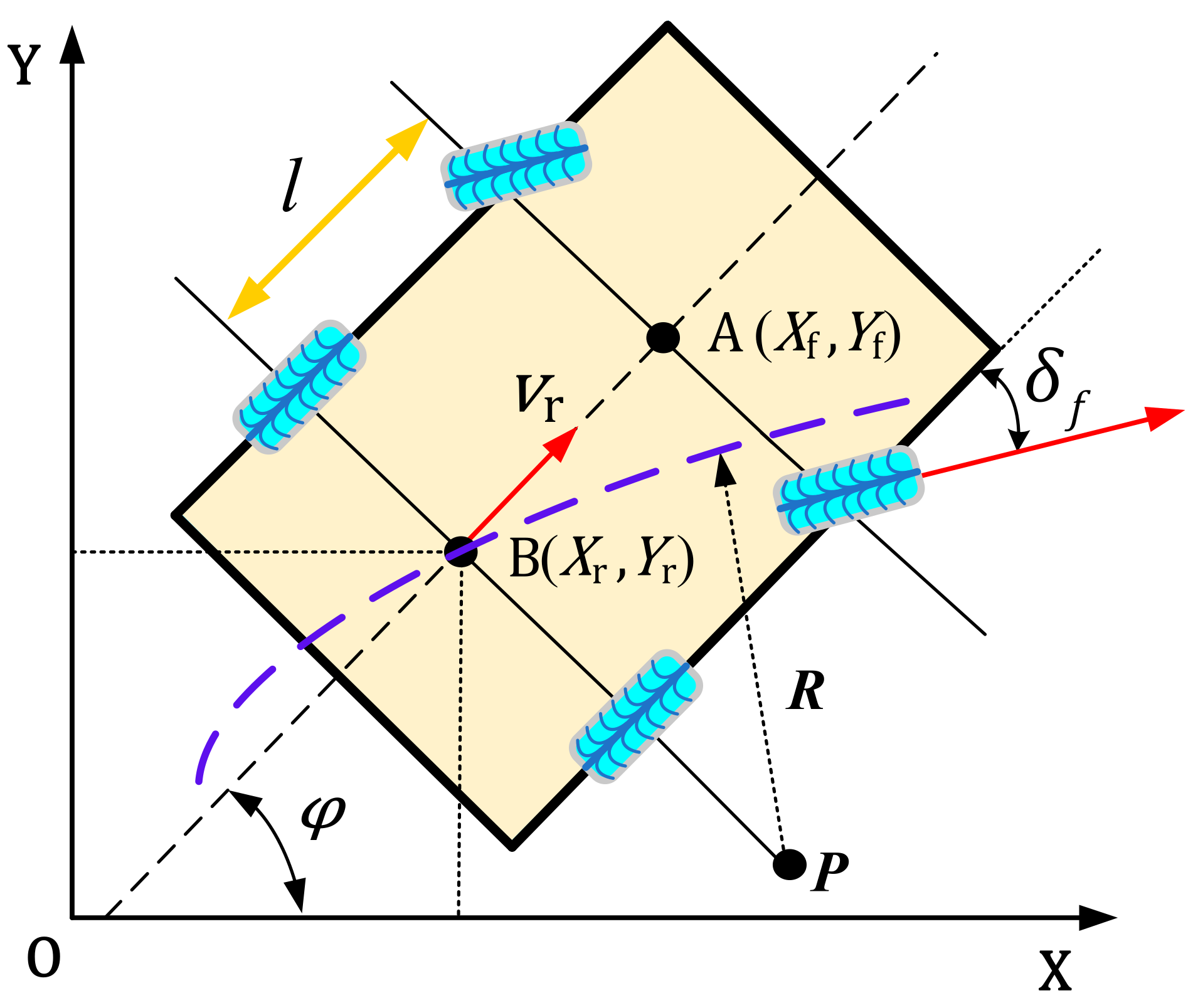
2. The Unmanned Vehicle’s Kinematics Model
3. Design of Nonlinear Model Predictive Control
3.1. Establishment of Nonlinear Prediction Model
3.2. Formulation of Objective Function
4. Simulation Verification
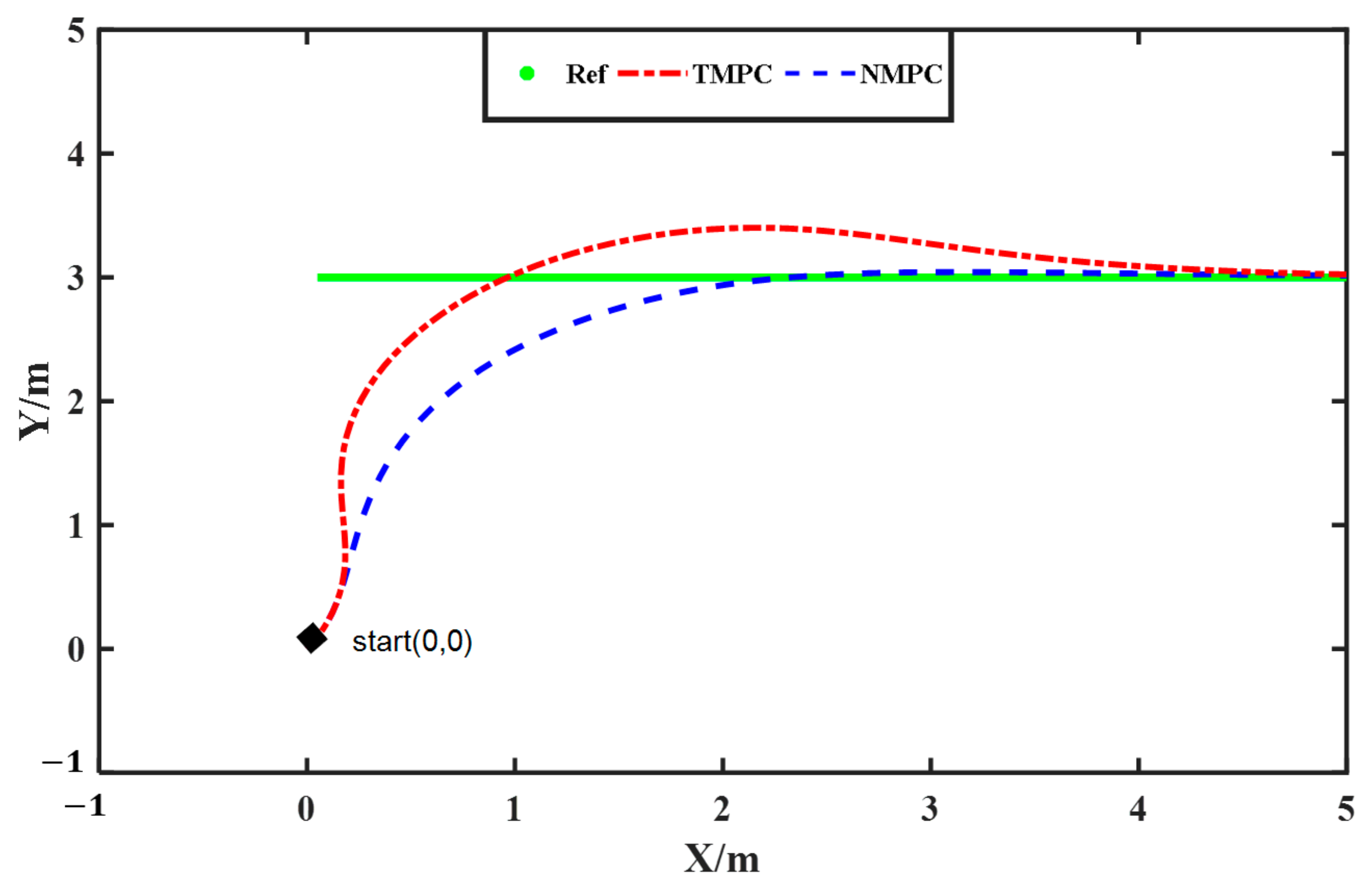
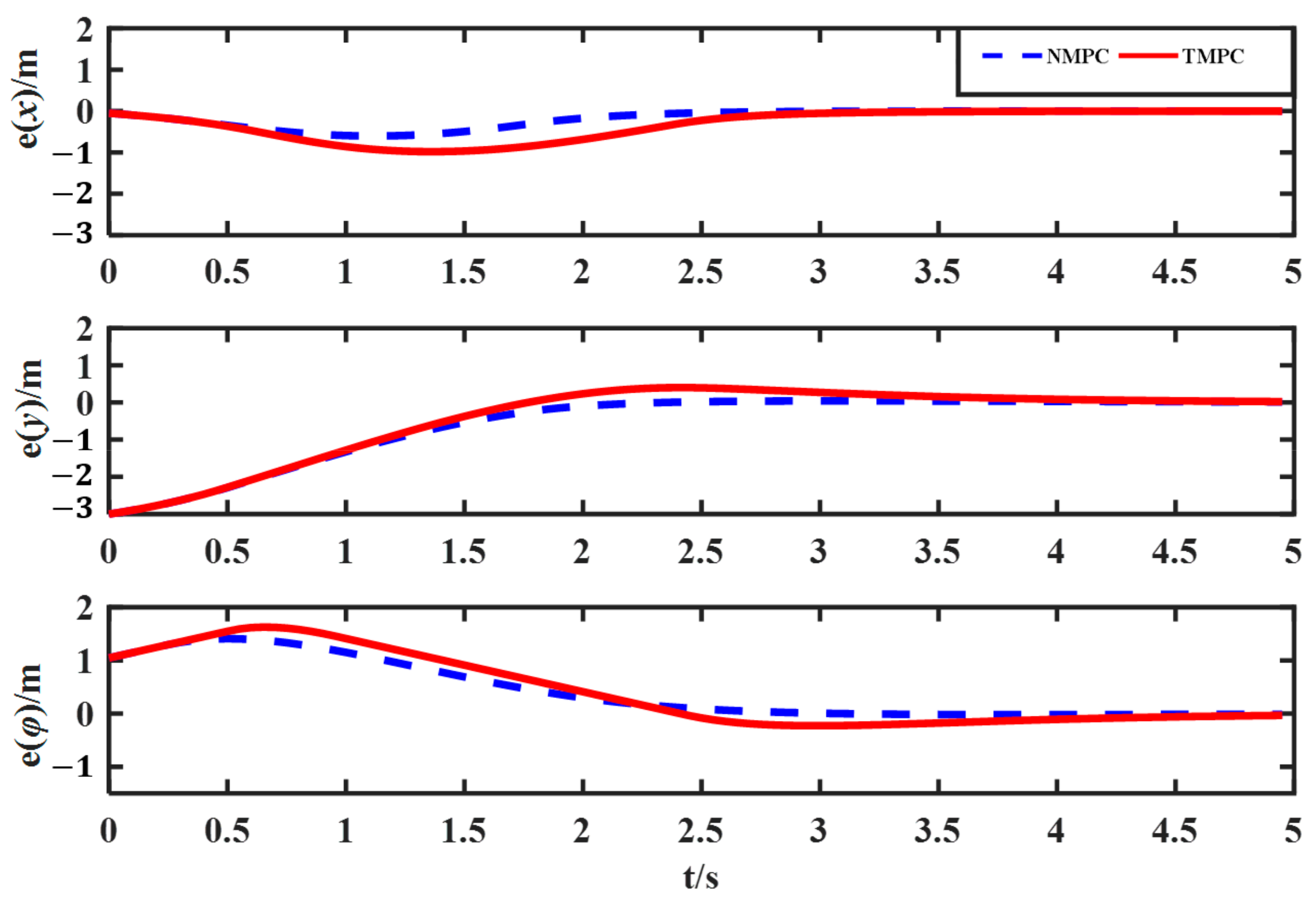
4.1. Simulations under a Straight-Line Trajectory
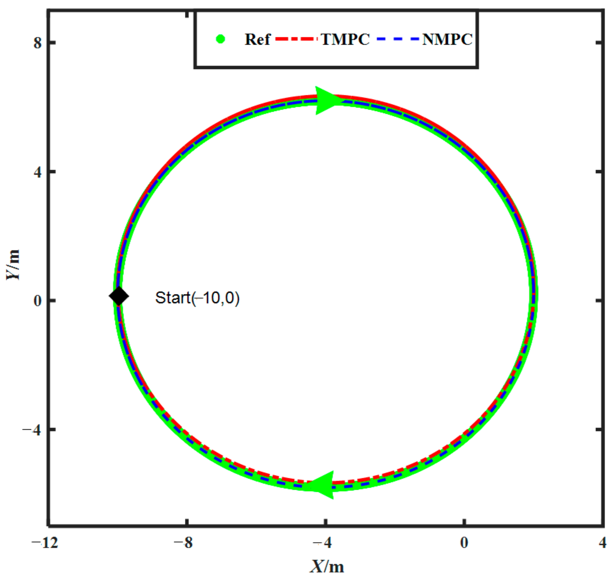
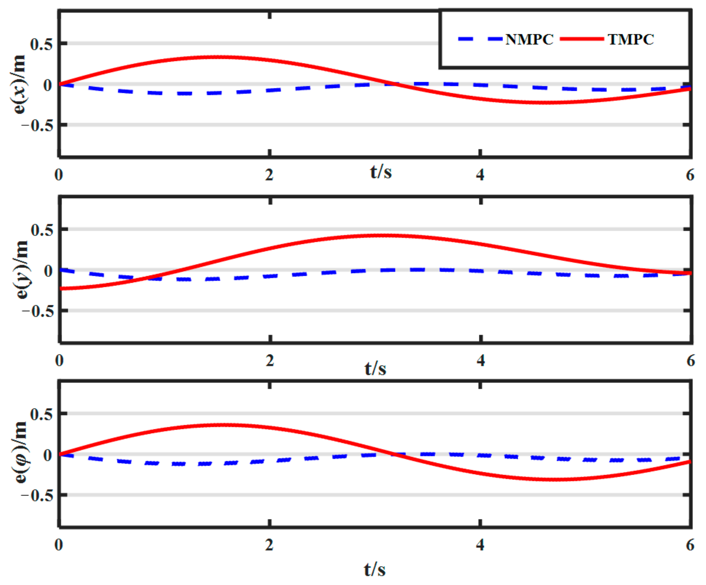
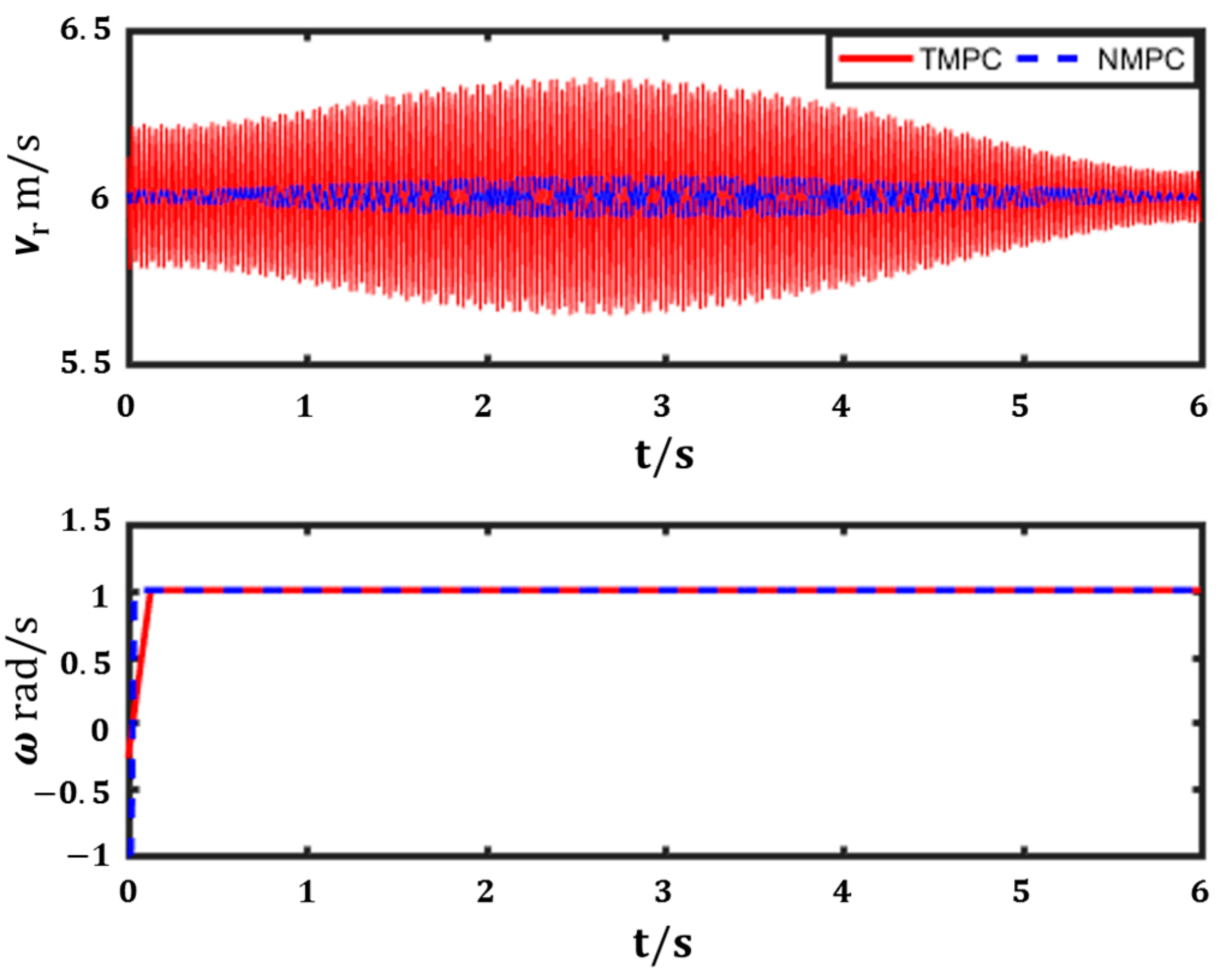
4.2. Simulations under a Single-Circle Trajectory
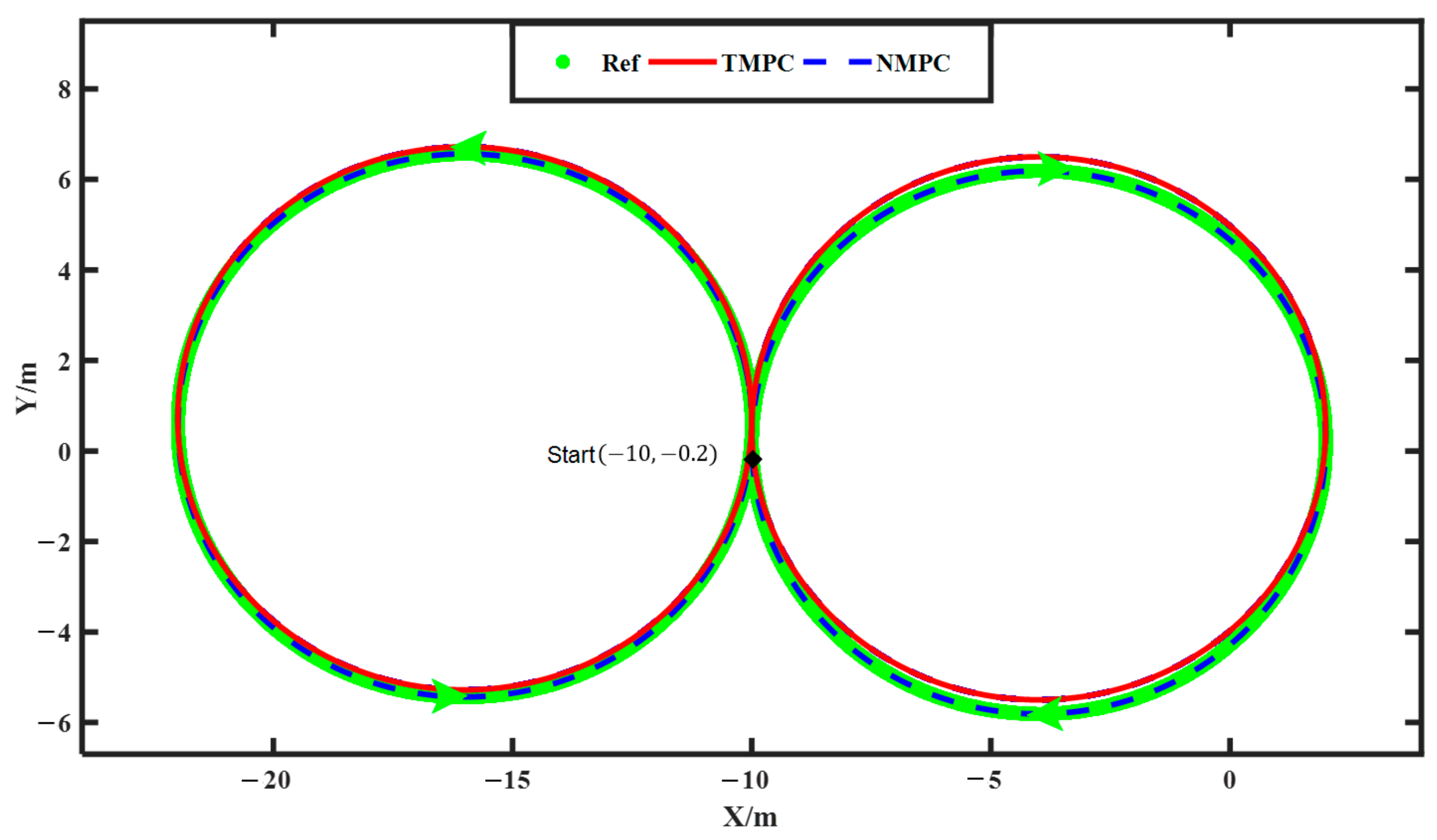
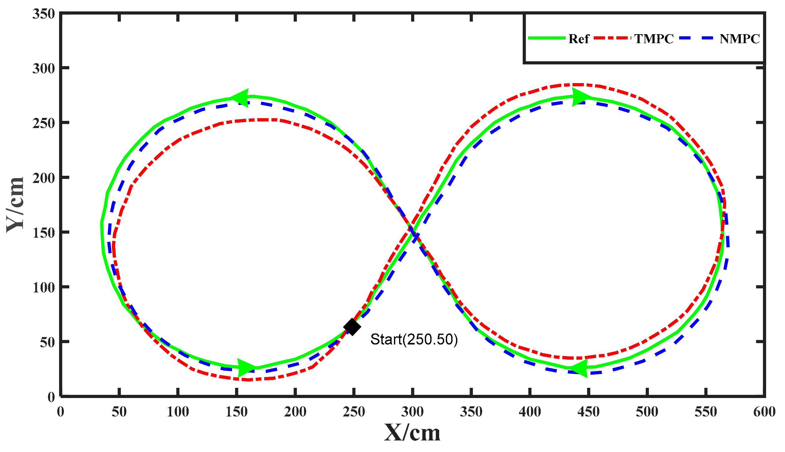
4.3. Simulations under a Twin-Circle Trajectory
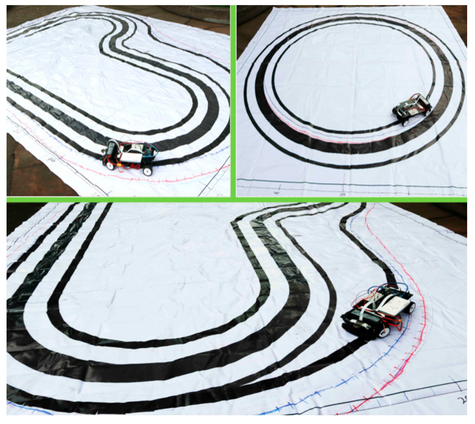
5. Field Test Verification
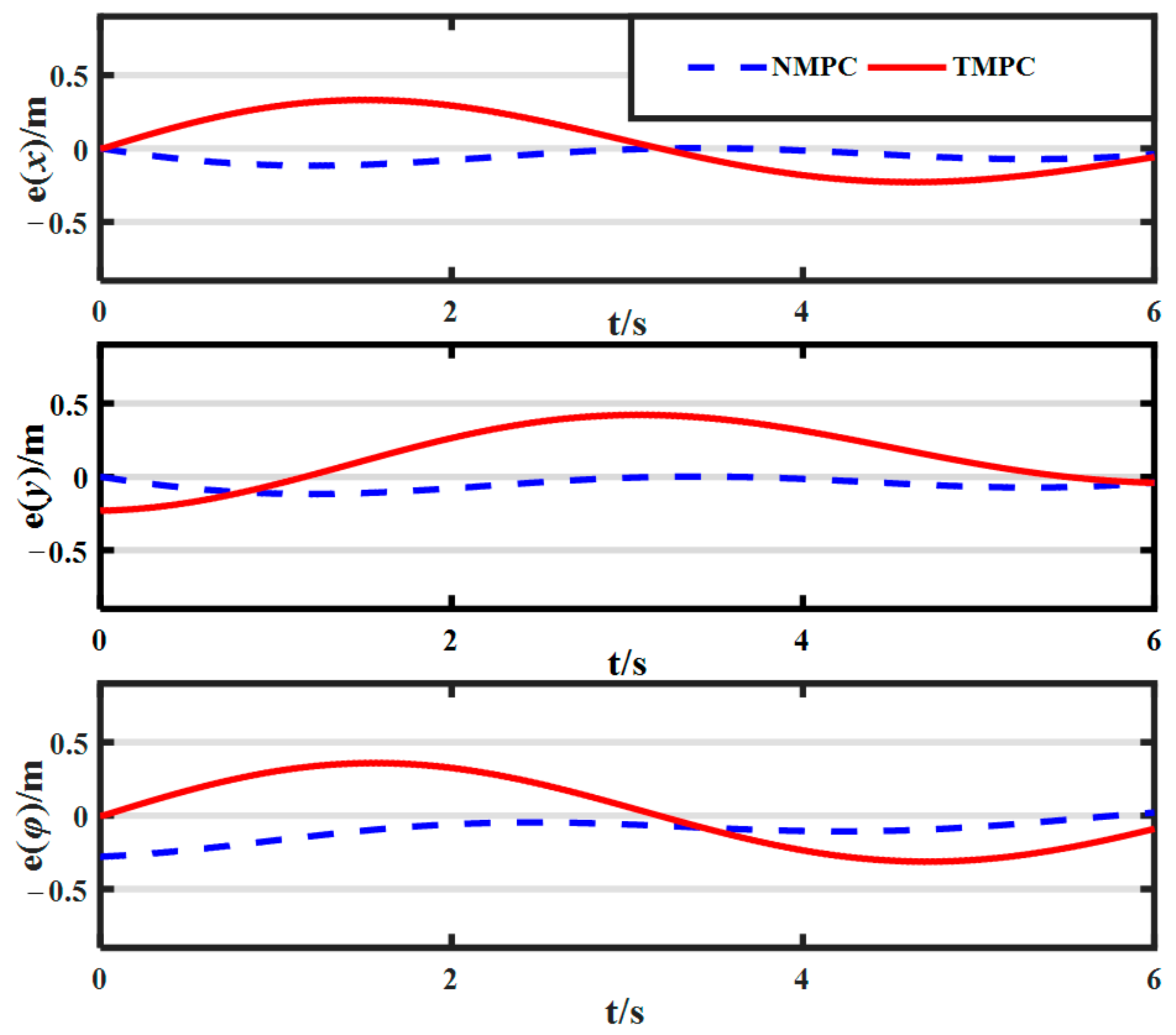
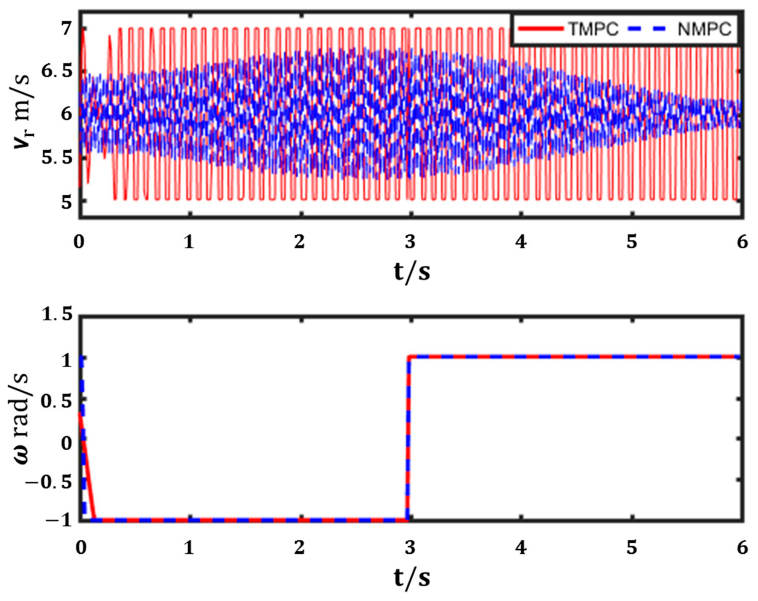
5.1. Test on Irregular Road
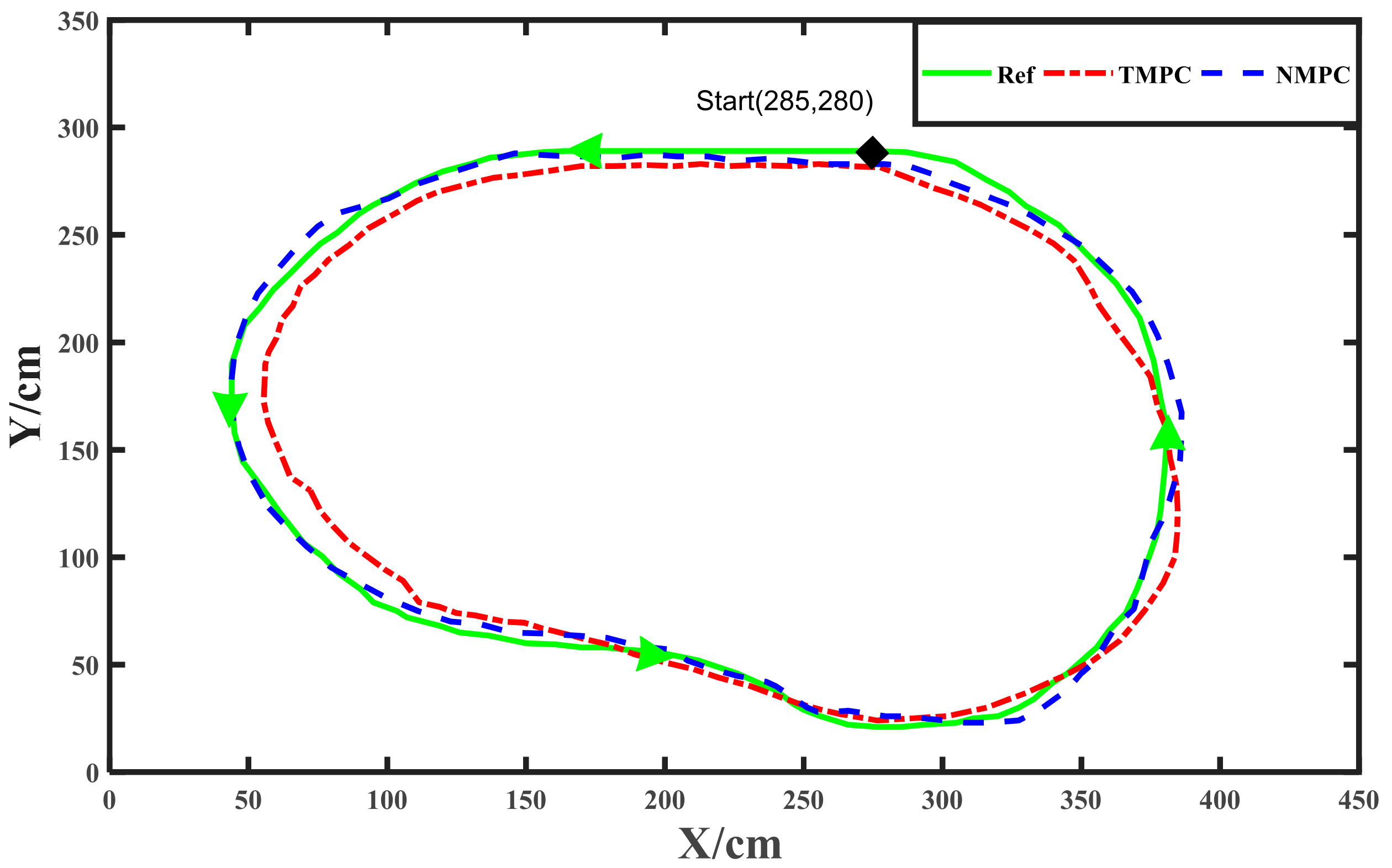
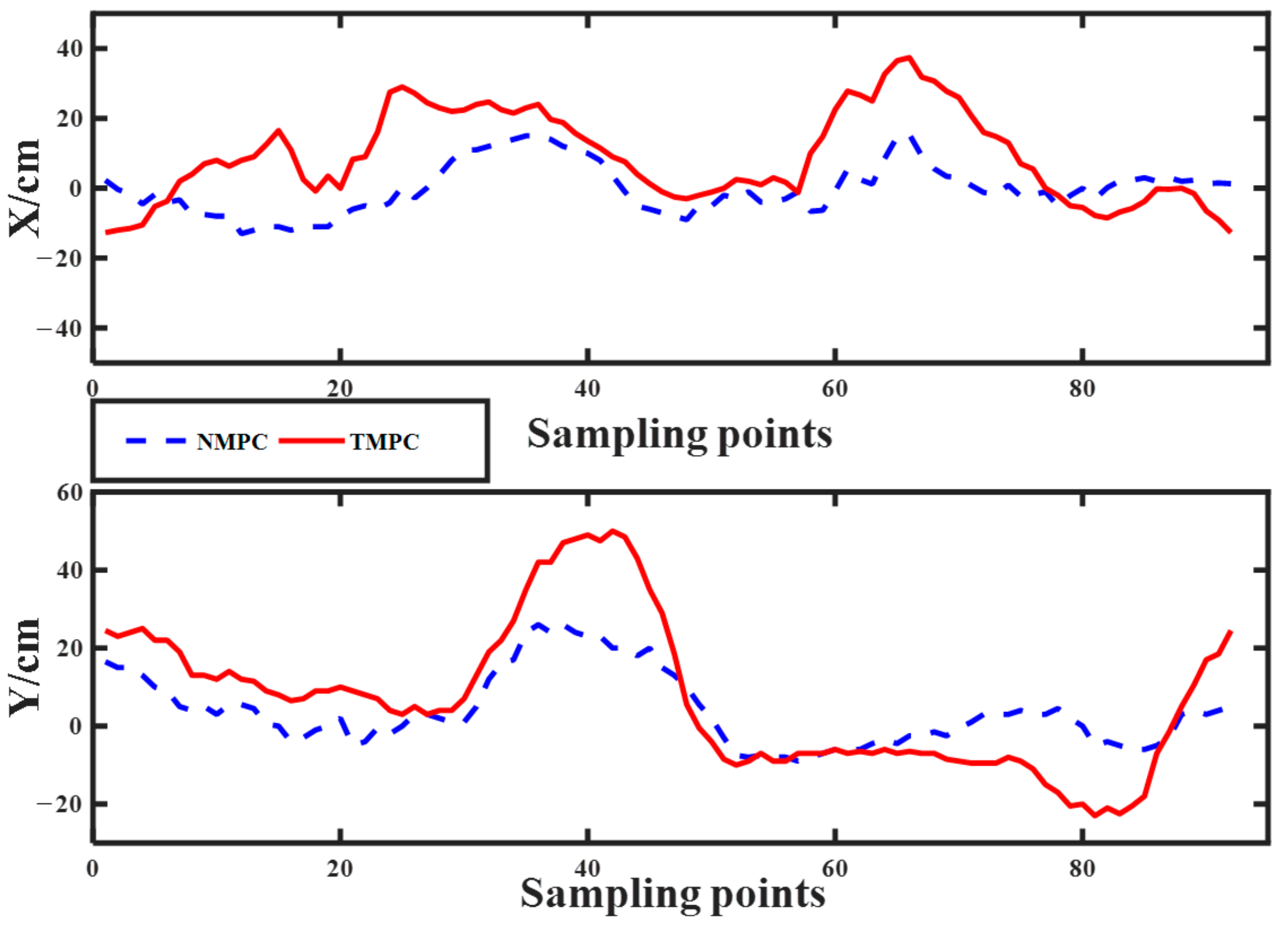
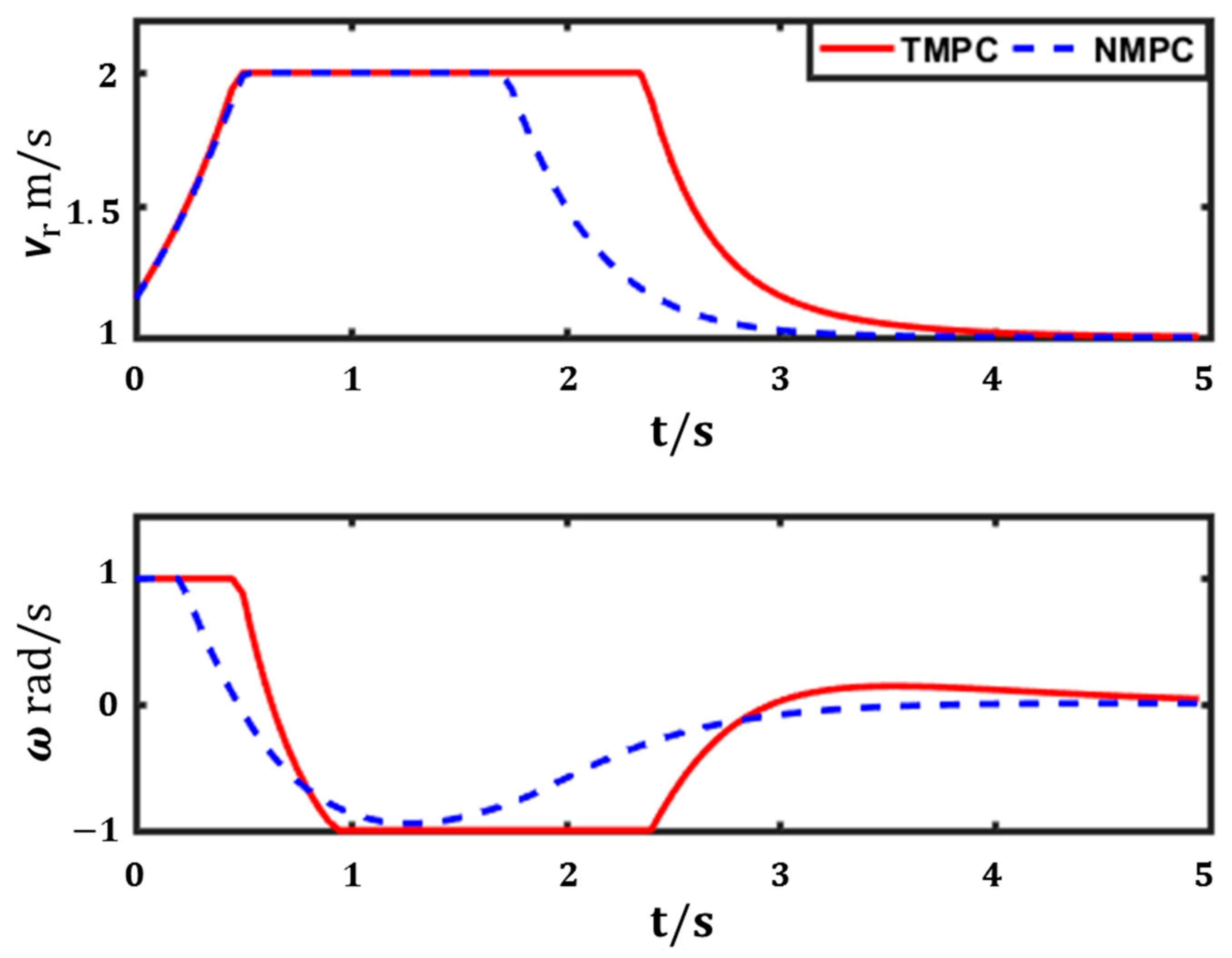
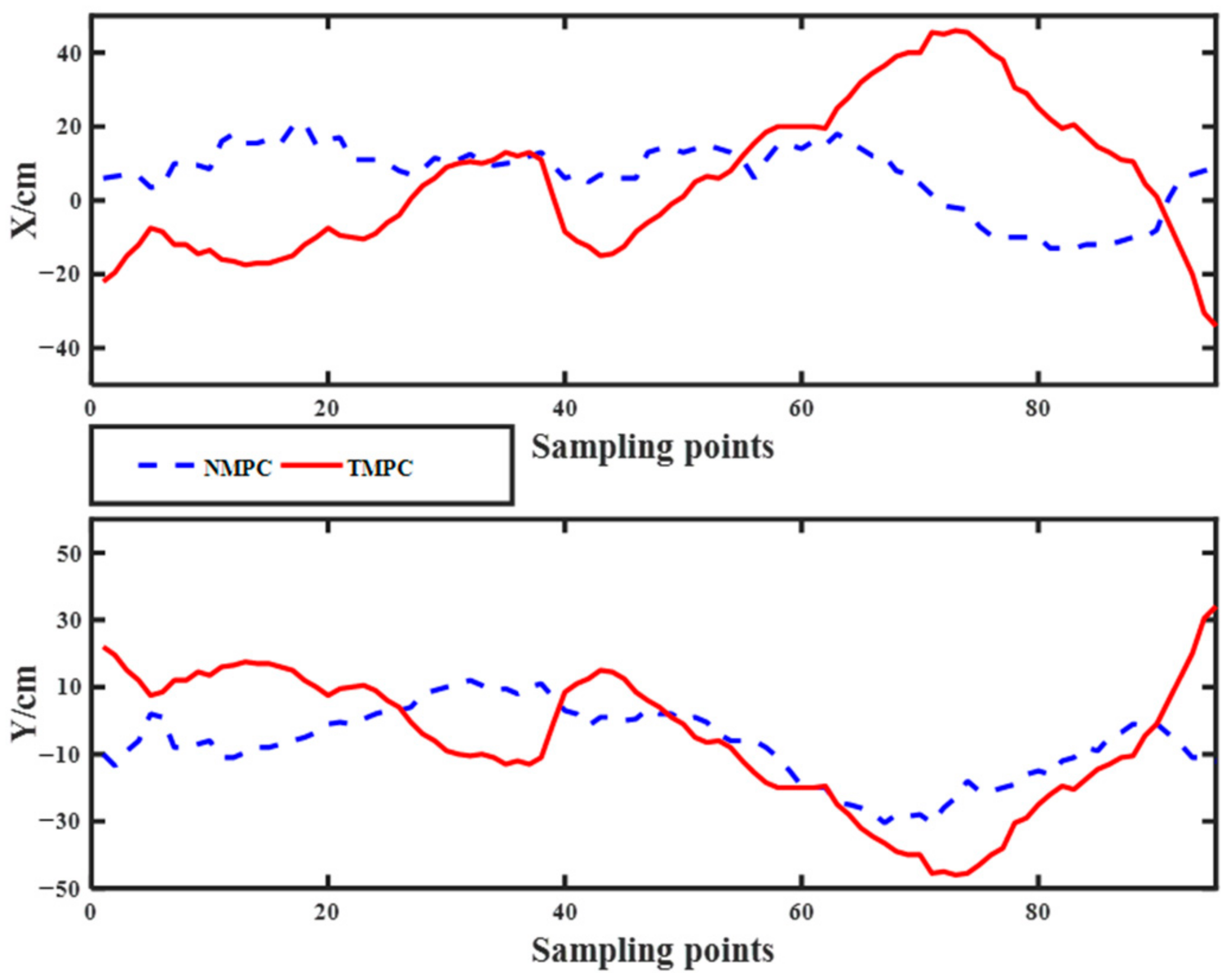
5.2. Test on Double-Circle Road
6. Conclusions
Author Contributions
Funding
Conflicts of Interest
References
- Lin, Y.C.; Lin, C.L.; Huang, S.T.; Kuo, C.H. Implementation of an Autonomous Overtaking System Based on Time to Lane Crossing Estimation and Model Predictive Control. Electronics 2021, 10, 2293. [Google Scholar] [CrossRef]
- Hu, C.; Qin, Y.; Cao, H. Lane keeping of autonomous vehicles based on differential steering with adaptive multivariable super-twisting control. Mech. Syst. Signal Process. 2019, 125, 330–346. [Google Scholar] [CrossRef]
- Wang, Z.; Wang, J. Ultra-local model predictive control: A model-free approach and its application on automated vehicle trajectory tracking. Control Eng. Pract. 2020, 101, 104482. [Google Scholar] [CrossRef]
- Wang, R.; Jing, H.; Hu, C. Robust H∞ path following control for autonomous ground vehicles with delay and data dropout. IEEE Trans. Intell. Transp. Syst. 2016, 17, 2042–2050. [Google Scholar] [CrossRef]
- Wang, Y.; Gao, S.; Chu, H.; Wang, X. Planning of Electric Taxi Charging Stations Based on Travel Data Characteristics. Electronics 2021, 10, 1947. [Google Scholar] [CrossRef]
- Li, J.; Xu, B.; Yang, Y. Three-phase qubits-based quantum ant colony optimization algorithm for path planning of automated guided vehicles. Int. J. Robot. Autom. 2019, 34, 156–163. [Google Scholar] [CrossRef]
- Ma, Y.; Hu, M.; Yan, X. Multi-objective path planning for unmanned surface vehicle with currents effects. ISA Trans. 2018, 75, 137–156. [Google Scholar] [CrossRef]
- Hu, L.; Gu, Z.Q.; Huang, J. Research and realization of optimum route planning in vehicle navigation systems based on a hybrid genetic algorithm. Proc. Inst. Mech. Eng. Part D J. Automob. Eng. 2008, 222, 757–763. [Google Scholar] [CrossRef]
- Chalvet, V.; Haddab, Y.; Lutz, P. Trajectory planning for micromanipulation with a non-redundant digital microrobot: Shortest path algorithm optimization with a hypercube graph representation. J. Mech. Robot. 2016, 8, 021013. [Google Scholar] [CrossRef]
- Ambike, S.; Schmiedeler, J.P.; Stanišić, M.M. Trajectory tracking via independent solutions to the geometric and temporal tracking subproblems. J. Mech. Robot. 2011, 3, 021008. [Google Scholar] [CrossRef]
- Jeong, Y.; Yim, J. Model Predictive Control-Based Integrated Path Tracking and Velocity Control for Autonomous Vehicle with Four-Wheel Independent Steering and Driving. Electronics 2021, 10, 2812. [Google Scholar] [CrossRef]
- Huang, Y.; Ding, H.; Zhang, Y. A motion planning and tracking framework for autonomous vehicles based on artificial potential field elaborated resistance network approach. IEEE Trans. Ind. Electron. 2019, 67, 1376–1386. [Google Scholar] [CrossRef]
- Yang, J.A.; Kuo, C.H. Integrating Vehicle Positioning and Path Tracking Practices for an Autonomous Vehicle Prototype in Campus Environment. Electronics 2021, 10, 2703. [Google Scholar] [CrossRef]
- Schwarting, W.; Alonso-Mora, J.; Paull, L. Safe nonlinear trajectory generation for parallel autonomy with a dynamic vehicle model. IEEE Trans. Intell. Transp. Syst. 2017, 19, 2994–3008. [Google Scholar] [CrossRef] [Green Version]
- Guo, H.; Liu, F.; Xu, F. Nonlinear model predictive lateral stability control of active chassis for intelligent vehicles and its FPGA implementation. IEEE Trans. Syst. Man Cybern. Syst. 2017, 49, 2–13. [Google Scholar] [CrossRef]
- Bujarbaruah, M.; Zhang, X.; Borrelli, F. Adaptive MPC with chance constraints for FIR systems. In Proceedings of the Annual American Control Conference, Milwaukee, WI, USA, 27–29 June 2018. [Google Scholar]
- Kim, E.; Kim, J.; Sunwoo, M. Model predictive control strategy for smooth path tracking of autonomous vehicles with steering actuator dynamics. Int. J. Automot. Technol. 2014, 15, 1155–1164. [Google Scholar] [CrossRef]
- Shen, C.; Guo, H.; Liu, F. MPC-based path tracking controller design for autonomous ground vehicles. In Proceedings of the 36th Chinese Control Conference, Dalian, China, 26–28 July 2017. [Google Scholar]
- Law, C.K.; Dalal, D.; Shearrow, S. Robust model predictive control for autonomous vehicles/self driving Cars. arXiv 2018, arXiv:1805.08551. [Google Scholar]
- Piga, D.; Formentin, S.; Bemporad, A. Direct data-driven control of constrained systems. IEEE Trans. Control Syst. Technol. 2017, 26, 1422–1429. [Google Scholar] [CrossRef] [Green Version]
- Pang, H.; Liu, N.; Hu, C.; Xu, Z. A practical trajectory tracking control of autonomous vehicles using linear time-varying MPC method. Proc. Inst. Mech. Eng. Part D J. Automob. Eng. 2022, 236, 709–723. [Google Scholar] [CrossRef]
- Chen, Y.; Hu, C.; Wang, J. Human-centered trajectory tracking control for autonomous vehicles with driver cut-in behavior prediction. IEEE Trans. Veh. Technol. 2019, 68, 8461–8471. [Google Scholar] [CrossRef]
- Hang, P.; Huang, S.; Chen, X. Path planning of collision avoidance for unmanned ground vehicles: A nonlinear model predictive control approach. Proc. Inst. Mech. Eng. Part I J. Syst. Control Eng. 2021, 235, 222–236. [Google Scholar] [CrossRef]
- Guerreiro, B.J.; Silvestre, C.; Cunha, R. Trajectory tracking nonlinear model predictive control for autonomous surface craft. IEEE Trans. Control Syst. Technol. 2014, 22, 2160–2175. [Google Scholar] [CrossRef]
- Shen, C.; Buckham, B.; Shi, Y. Modified C/GMRES algorithm for fast nonlinear model predictive tracking control of AUVs. IEEE Trans. Control Syst. Technol. 2016, 25, 1896–1904. [Google Scholar] [CrossRef]
- Guo, N.; Lenzo, B.; Zhang, X. A real-time nonlinear model predictive controller for yaw motion optimization of distributed drive electric vehicles. IEEE Trans. Veh. Technol. 2020, 69, 4935–4946. [Google Scholar] [CrossRef] [Green Version]
- Kuhne, F.; Lages, W.F.; da Silva, J.G., Jr. Model predictive control of a mobile robot using linearization. Proc. Mechatron. Robot. 2004, 4, 525–530. [Google Scholar]
- Pang, H.; Zhang, X.; Yang, J. Adaptive backstepping-based control design for uncertain nonlinear active suspension system with input delay. Int. J. Robust Nonlinear Control 2019, 29, 5781–5800. [Google Scholar] [CrossRef]


| Symbol | Description | Symbol | Description |
|---|---|---|---|
| The center of the front axle | l | The distance from point A to B | |
| The center of the rear axle | ω | The yaw rate of UV | |
| The deflection angle of the front axle | The yaw angle of UV | ||
| The forward speed of point B |
| Type | |||
|---|---|---|---|
| TMPC | 0.559 | 1.11 | 0.8264 |
| NMPC | 0.2731 (↓51.14%) | 1.095 (↓1.35%) | 0.6763 (↓18.16%) |
| Type | |||
|---|---|---|---|
| TMPC | 0.2208 | 0.3734 | 0.2515 |
| NMPC | 0.1210 (↓45.20%) | 0.2284 (↓40.44%) | 0.1285 (↓48.95%) |
| Type | |||
|---|---|---|---|
| TMPC | 0.1622 | 0.2743 | 0.1848 |
| NMPC | 0.0562 (↓65.35%) | 0.1245 (↓54.61%) | 0.0543 (↓71.10%) |
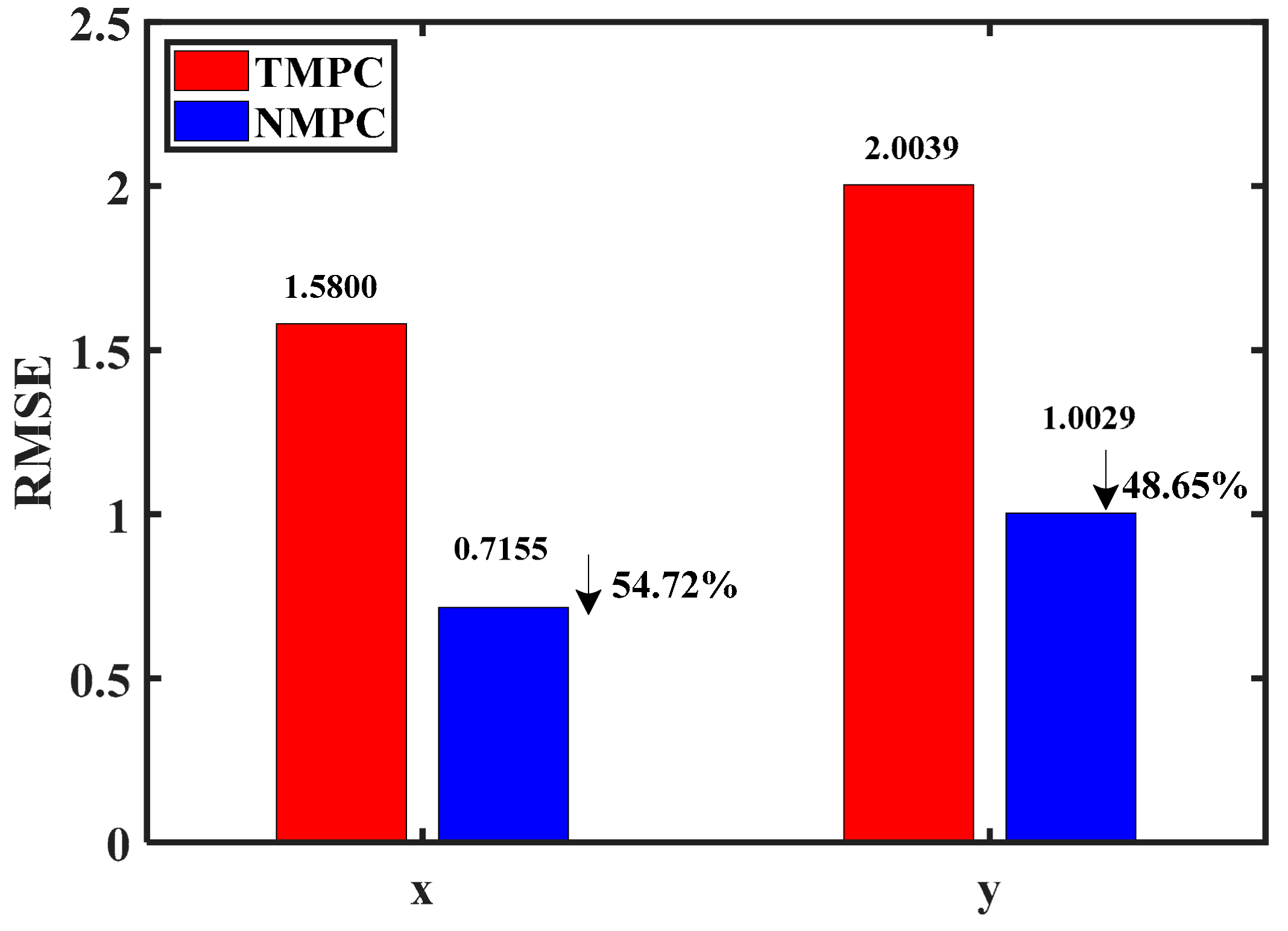
| Type | ||
|---|---|---|
| TMPC | 1.5800 | 2.0039 |
| NMPC | 0.7155 (↓54.72%) | 1.0029 (↓48.65%) |
| Type | ||
|---|---|---|
| TMPC | 2.7814 | 2.8215 |
| NMPC | 1.2061 (↓56.63%) | 1.4465 (↓48.73%) |
Publisher’s Note: MDPI stays neutral with regard to jurisdictional claims in published maps and institutional affiliations. |
© 2022 by the authors. Licensee MDPI, Basel, Switzerland. This article is an open access article distributed under the terms and conditions of the Creative Commons Attribution (CC BY) license (https://creativecommons.org/licenses/by/4.0/).
Share and Cite
Pang, H.; Liu, M.; Hu, C.; Liu, N. Practical Nonlinear Model Predictive Controller Design for Trajectory Tracking of Unmanned Vehicles. Electronics 2022, 11, 1110. https://doi.org/10.3390/electronics11071110
Pang H, Liu M, Hu C, Liu N. Practical Nonlinear Model Predictive Controller Design for Trajectory Tracking of Unmanned Vehicles. Electronics. 2022; 11(7):1110. https://doi.org/10.3390/electronics11071110
Chicago/Turabian StylePang, Hui, Minhao Liu, Chuan Hu, and Nan Liu. 2022. "Practical Nonlinear Model Predictive Controller Design for Trajectory Tracking of Unmanned Vehicles" Electronics 11, no. 7: 1110. https://doi.org/10.3390/electronics11071110
APA StylePang, H., Liu, M., Hu, C., & Liu, N. (2022). Practical Nonlinear Model Predictive Controller Design for Trajectory Tracking of Unmanned Vehicles. Electronics, 11(7), 1110. https://doi.org/10.3390/electronics11071110