Abstract
This paper investigates the use of approximate fixed-width and static segment multipliers in the design of Delayed Least Mean Square (DLMS) adaptive filters based on the sign–magnitude representation for the error signal. The fixed-width approximation discards part of the partial product matrix and introduces a compensation function for minimizing the approximation error, whereas the static segmented multipliers reduce the bit-width of the multiplicands at runtime. The use of sign–magnitude representation for the error signal reduces the switching activity in the filter learning section, minimizing power dissipation. Simulation results reveal that, by properly sizing the two approaches, a steady state mean square error practically unchanged with respect to the exact DLMS can be achieved. The hardware syntheses in a 28 nm CMOS technology reveal that the static segmented multipliers perform better in the learning section of the filter and are the most efficient approach to reduce area occupation, while the fixed-width multipliers offer the best performances in the finite impulse response section and provide the lowest power dissipation. The investigated adaptive filters overcome the state-of-the-art, exhibiting an area and power reduction with respect to the standard implementation up to −18.0% and −64.1%, respectively, while preserving the learning capabilities.
1. Introduction
Adaptive filters are widely used in many application fields such as telecommunication, biomedical, acoustic, video and image processing, and can solve problems such as system identification, channel equalization, noise, and echo cancellation [1]. Among the different applications, they reduce the noise in the electrocardiograms due to muscle motion and respiration rate [2,3], or can improve the receiver sensitivity in modern transceivers [4,5]. In [6], an adaptive filter performs a noise cancellation for the detection of radar signals; the works [7,8,9] describe variable step-size techniques for the suppression of the echo in the acoustic systems.
The simple hardware structure and the favorable convergence properties make the Least Mean Square (LMS) algorithm the most used adaptive filter. The LMS algorithm changes its impulse response at runtime with the aim to minimize the mean square error (MSE) between its own output and an external reference solicitation (generally named desired output). As shown in Figure 1, a finite impulse response (FIR) section computes the filter output y(n), whereas a subtraction between the desired output d(n) and y(n) produces the error signal e(n). Then, a learning block computes the gradient of the MSE, given by the multiplication between e(n) and the input samples, with the aim to update the coefficients and to minimize the error signal in a mean-square sense.
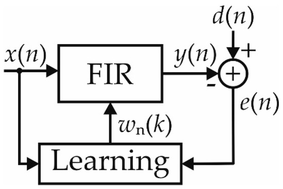
Figure 1.
Simplified scheme of the Least Mean Square algorithm.
Since the FIR section and the learning process require an intensive usage of multipliers, adders, and registers, the adoption of low-power and low-area techniques is of paramount importance for achieving a feasible implementation of the algorithm.
In the literature, several designs have been proposed. In [10], the FIR section and the learning block share the same multipliers in order to reduce the area occupation at the cost of double the operative frequency. In addition, the paper shows that the direct form of the filter performs better than the transpose form counterpart since it requires a lower number of registers, exhibits a comparable critical path delay, and offers a reduced convergence time. The adoption of pipelined versions of the LMS algorithm, generally referred to as Delayed LMS (DLSM), also improves the implementation at the cost of a change in the learning rule [11,12,13,14,15,16]. For instance, the introduction of a register between the FIR section and the learning block allows us to shorten the critical path of the filter and to relax the timing constraints during the design. In addition, the pipeline also prevents glitch propagation from the FIR to the learning block and allows a reduction in energy dissipation. In [12], the FIR part involves a binary tree adder that simplifies the introduction of pipeline levels for high-speed applications, as well as a proper encoding on the input samples, which is proposed to reduce the complexity of the multiplications. The works [13,14,15,16] trade the hardware complexity with the convergence rate of the DLMS by applying a correction term to the updating formula.
Since the multiplications are power-hungry operations, a proper design of the binary multipliers helps in improving the hardware performances of the adaptive filter. In this contest, the works [17,18,19,20] exploit the Distributed Arithmetic (DA) paradigm for the realization of the arithmetic circuits in the LMS-based filters. Here, Look-Up Tables (LUTs) and shift and add operations substitute the multipliers of the FIR and the learning sections. Since LUT size is a critical design parameter, proper coding schemes (as offset binary coding, radix-r, or canonic sign digit) are used for representing the signals stored in the LUTs [17,19]. The design described in [18] introduces additive logic for reducing the number of LUTs used for the updating, as well as the work [19] proposes a register-based approach instead of a LUT-based method. In [20], the approximate Booth multiplier of [21] is used both in the FIR and in the learning sections, whereas the partial products in the FIR part are added in a shift-and-add fashion.
Approximate computing approaches [22,23], which trade precision of calculation to achieve better electrical performances, are a valuable means for improving the performances of error-resilient circuits and, as a consequence, are potentially employable in the design of adaptive filters. With reference to approximate multipliers, approximations can be introduced during the computation of the partial products, in the compression stage of the Partial Product Matrix (PPM), or in the final carry propagate adder [24,25,26,27,28,29,30,31,32,33,34,35]. For instance, the works [26,27,28] propose the usage of approximate compressors for the reduction in the PPM. The fixed-width multiplier techniques are characterized by not forming the least significant columns of the PPM [31,32,33,34,35] in order to improve area occupation and power dissipation. While [32] proposes a constant compensation term for recovering the quality of results, the designs described in [33] and in [34] properly modify the PPM in order to minimize the maximum absolute error and the MSE of the approximation, respectively. A different approach is the Static Segment Method (SSM) [36], where multipliers inputs are segmented in order to allow the employ of a multiplier with a reduced number of input bits. In this case, since the approximation is introduced only for inputs that are large in magnitude, the approach tends to provide a good relative error.
The papers [37,38] study the performances of the LMS filter with different approximate multipliers. Results show that a proper choice of the multiplier architecture is required in order to ensure the convergence of the algorithm. In addition, a modified version of the multiplier described in [28] is proposed in which OR gates reduce the least significant part of the PPM while minimizing the error probability. In [39], a control circuit reduces the switching activity of the signals approximating to zero the smallest coefficients, whereas the design [40] scales the precision of the input samples in the learning block at runtime for the gradient computation. In this case, since the approximation error depends on e(n) (that is close to zero at regime), the convergence properties of the algorithm are practically unchanged if compared with the standard implementation. The paper [41] further improves the approach of [40] by using the absolute value of the error signal for the gradient computation and proposes a novel sign–magnitude multiplier able to combine the absolute value of the error with the rounded inputs in the feedback. Although results reveal a remarkable reduction in the power consumption without degrading the regime MSE, the logic used for the rounding and the sign–magnitude representation causes a sensible increase in the area occupation.
In this paper, we propose novel implementations for the DLMS filter based on the sign–magnitude error representation by using approximate multiplier techniques. To the best of the authors’ knowledge, this is the first paper exploring the possibility of computing the gradient signal by combining the sign–magnitude technique with approximate multipliers.
Following an approach similar to [41], the technique proposed in this paper exploits the absolute value of the error for the coefficient updating. Since the module of the error is near zero at regime, its MSBs are low, and this can be exploited to reduce the switching activity of the multipliers in the learning block. Starting from this topology, the paper studies the use of approximate multipliers to further improve circuit performances. Two approaches are investigated: the fixed-width technique (by considering the optimal MSE solution of [34]) and the SSM technique, both modified and customized for the particular application. Both approaches are applied to the learning section of the filter. In addition, a solution employing the fixed-width technique in the FIR section of the filter is also proposed and analyzed.
It is worth noting that we choose to approximate the DLMS algorithm in order to compare the performances with the competitive work of [41] (that implements a DLMS updating rule); however, the proposed techniques can be used to improve the hardware performances of any LMS-based adaptive filter (as, for instance, the design of [42]).
Results, obtained by means of post-synthesis simulations in TSMC 28 nm CMOS technology, show that the proposed implementations outperform the state-of-the-art and achieve a steady-state MSE comparable to the standard case. The SSM technique results in the most effective approach when area occupation is the most important design parameter, whereas the fixed-width technique gives the lowest power dissipation.
The paper is organized as follows: Section 2 briefly recalls the DLMS algorithm and the sign–magnitude error technique, and, afterwards, describes the application of the fixed-width and SSM approximations to the DLMS filter. Section 3 presents the implementation results for a CMOS 28 nm technology. Section 4 compares the regime and hardware performances with the state-of-the-art. Finally, Section 5 concludes the paper.
2. Materials and Methods
2.1. Delayed LMS Algorithm
Figure 2 depicts the detailed block diagram of the DLMS filter with one pipeline level on the error signal. As shown in the figure, the FIR section exploits an input buffer (dashed red rectangle) that acquires the input x(n), whereas a bank of multipliers and an adder tree realize the sum of products for the computation of the output y(n); therefore, defining N as the filter dimension, x(n − k) as the k-th acquired input sample, with k = 0, 1,…N − 1, and wn(k) as the k-th coefficient at the iteration n, the following relation holds for the output computation [1]:
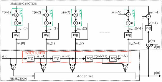
Figure 2.
Block diagram of the DLMS filter.
It is worth noting that the coefficients depend on the time index n since they change iteration by iteration during the learning process.
The error signal e(n) is computed by comparing y(n) with the desired output d(n) as follows:
whereas the delayed error is used for the computation of the k-th component of the MSE gradient G(k):
Then, the learning formula, realized by means of the Multiply-And-Accumulate (MAC) structure depicted in the green dashed rectangle, updates the coefficients as follows [1]:
In (4), µ is the step-size parameter that handles the trade-off between the convergence time and the quality of regime MSE. Indeed, the lower the step size, the better the regime MSE, the slower the updating process.
Since Equation (3) approximates the computation of the MSE gradient, the DLMS algorithm performs a noisy adaptation of the coefficients [1].
In the case in which Δ pipeline stages are used (as in [13,14,15,16]), Equation (3) becomes
The introduction of sophisticated pipelines schemes (as, for instance, in the adder tree) helps in improving the speed of the circuit but leads to a sensible increase in the area and power; therefore, in the following, we consider only a single pipeline stage between the FIR and the learning section.
2.2. Sign–Magnitude Error Representation
As observable by Equations (3) and (4), and Figure 2, the learning algorithm requires N MAC blocks for computing the coefficients. Since in steady-state conditions, the error signal is very close to zero, the noisy nature of the adaptive process allows the error signal to oscillate between positive and negative values continuously. Accordingly, the MSBs of the error vary between the high and the low logic states in subsequent cycles, thus increasing switching activity and power consumption in all the MAC structures.
Using the absolute value of the error signal for the gradient computation allows reducing the power consumption in the filter. Indeed, since the absolute value |e(n − 1)| is very small and always positive at regime, its MSBs are stuck at zero and reduce the switching activity of all the MAC blocks. Accordingly, the power consumption also drops.
The absolute value |e(n − 1)| is computed by inverting the bits of the error when its sign is negative and considering the addition of a further bit with the least significant weight of e(n − 1) to correctly compute the 2’s complement. In the case of an error with a negative sign, the sign of the error is recovered in the computation of G(k) (see (3)) by changing the sign of x(n – k − 1).
Figure 3 shows the scheme of the DLMS when the sign–magnitude technique is used for the coefficient updating. In the figure, we indicate with pe and px the number of bits of the error signal and of the input samples. Similarly, we indicate with pw and pw_fir the number of bits of the coefficients at the output of the MAC block and after the rounder R in the FIR section, respectively. As well known, the usage of pw > pw_fir bits for the coefficients at the output of the MAC improves the quality of the learning and optimizes the regime MSE of the filter [43].
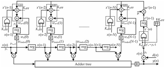
Figure 3.
Block diagram of the DLMS filter with sign–magnitude technique. The dashed square with the XOR gate represents the XOR bank, whereas, in the learning, the dashed rectangles highlight the sign–magnitude (MS) MAC blocks.
An XOR bank applied on the signal e(n) performs the first step for the computation of |e(n − 1)|. Naming Ke the MSB of e(n), if Ke is low (i.e., e(n) is positive or zero), the XOR bank does not change the bits of the error signal. On the contrary, if Ke is high (i.e., e(n) is negative), the XOR bank inverts the bits of the error. Please note that the xor-ed error, e′(n), is expressed on p′e = pe − 1 bits since the MSB is always low. By taking into account the LSB that needs to be added to compute 2’s complement, we can conclude that |e(n − 1)| is related to the registered XOR output by means of the following relationship:
where KeFF is the registered value of Ke and e′(n − 1) is the registered version of the xor-ed error. We underline that, in order to simplify the discussion, in (6) the LSB of the error is assumed to have a weight equal to 20.
It is worth noting that the XOR bank is placed before the register that delays the error signal with the aim to prevent the glitch propagation toward the arithmetic circuits of the learning block.
As shown in Figure 3, when the error signal is negative (i.e., KeFF = 1), the correct sign of the gradient is recovered by using XOR banks to invert x(n − k − 1) signals. Again, by considering the LSB that needs to be added to compute 2’s complement, and indicating with x′(n − k − 1) the xor-ed input, the sign-changed version of x(n − k − 1), signal that we name xsc(n − k − 1), is related to the XOR bank output by the following relationship:
Further, in this case, we assumed that the LSB of the input has weight 20 for the sake of simplicity.
As a consequence, the gradient signal of (3) is computed as:
By substituting Equations (6)–(8) in (4), the expression that describes the operation that needs to be performed by the sign–magnitude (MS) MAC block is found:
As shown in (9), the learning rule with the sign–magnitude technique requires the product between e′(n − 1) and x′(n − k − 1), the addition with the coefficient at iteration n, and the addition with further terms that complete the module computation of the error signal and sign change of the input sample. Figure 4 represents the PPM of the MAC with the xor-ed error expressed on p′e = 7 bits and the input sample expressed on px = 5 bits. The coefficients are supposed on pw = 13 bits, whereas the step-size parameter is set to 1 to simplify the discussion (please note that in order to improve the hardware implementation, the step-size parameter is always chosen as a power of 2). In the figure, we have also assumed that the four MSBs of e′(n − 1) are zero in steady-state conditions and we have reported the corresponding terms that nullify in gray. This highlights that in these conditions, a large part of the PPM is stuck at zero, thus allowing a reduction in power consumption.
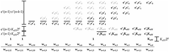
Figure 4.
Partial product matrix of the sign–magnitude MAC block. The gray partial products are zero thanks to the sign–magnitude technique.
2.3. Fixed-Width Approximation
2.3.1. Fixed-Width MAC Block in the Feedback
This section describes the employ of the fixed-width technique for the implementation of the MAC block in the learning section. We focus on the technique which optimizes the MSE proposed in [34]. Figure 5 recalls the fixed-width method in the case of an unsigned 8-bit multiplier. As it can be observed, the first 8 least significant columns form the least significant part of the PPM that, in turn, is divided into a Left-Most Portion (LMP) and a Right-Most Portion (RMP). The LMP includes h columns, whereas the RMP collects the remaining partial products. The parameter h can be chosen at design time to trade precision for circuit complexity. This technique preserves only the most significant column C* of RMP (highlighted in red) and the terms of the LMP, whereas the other partial products, depicted in blue, are discarded. The partial products of the C* are weighted to best approximate the dropped terms in the mean-square sense. For instance, in the case of Figure 5, the error compensation function promotes the central partial products b3a2 and b2a3 to the next column in the LMP and preserves the other ones in the original position (see [34]).
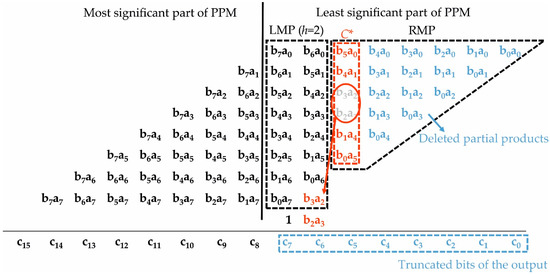
Figure 5.
Partial product matrix of the unsigned fixed-width multiplier proposed in [34]. In the figure, it is chosen h = 2.
Figure 6 represents the MAC block of (9) where the fixed-width technique is applied by reducing the bit-width at the output of the MAC of a quantity ptrunc. In the considered example we choose ptrunc = 5 and h = 1, and the coefficients are expressed on pw = 13 − ptrunc = 8 bits. Please note that the choice of ptrunc (that is, the choice of pw) can strongly impact the precision of the learning process also to avoid the stalling phenomenon of the adaptive filter (see [43]). Based on an extended set of simulations, we have verified that a good choice is setting pw = pw_fir + 7, which preserves very good precision. Note also that in Figure 6 we considered p′e = 7 bits for e′(n − 1), and px = 5 bits for x′(n − k − 1). The discarded partial products are highlighted in blue, and, as it can be observed, the bit KeFF and some of the terms e′iKeFF and x′iKeFF can also be dropped by using an approach similar to the fixed-width technique.
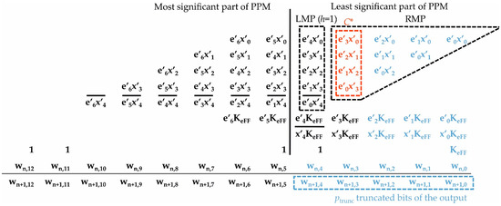
Figure 6.
MAC block with the fixed-width technique applied to the product e′(n − 1)∙x′(n − k − 1) and the truncation on e′(n − 1)∙KeFF20, x′(n − k − 1)∙KeFF20 and KeFF20.
It is worth highlighting that this approach, while reducing the circuit complexity (due to dropped terms), also has benefits in terms of power dissipation since it tends to cancel the less significant partial products of the PPM whose switching activity is not reduced by the sign–magnitude method; therefore, the two techniques tend to complete each other in order to reduce the power dissipation of the circuit. In addition, since the fixed-width approach reduces the number of bits of the coefficients in the learning section, it is also possible to reduce the bit width of the registers that store these coefficients with further beneficial effects on the hardware performances.
2.3.2. Fixed-Width Approximation in the FIR Section
In this paragraph, we also extend the usage of the fixed-width multiplication to the products of the FIR part. In the following, for the sake of simplicity, we assume that the input samples x(n − k) and the coefficients wrnd,n(k) are expressed on the same number of bits (that is px = pw_fir). Let us name ptrunc_fir as the number of bits truncated at the output of each fixed-width multiplier in the FIR section. Let us also name pround_fir as the number of bits that, in the implementation of Figure 3 using full-precision multipliers, are pruned by the rounder, which produces the filter output y(n). Assuming an LSB of weight 20, in the implementation with full-precision multipliers, the mean-square output error of the FIR section is given by:
The combined and asymptotic (for h → ∞) mean square error of all fixed-width multipliers in the FIR section is, on the other hand, given by:
If, for example, we impose:
we can derive a sizing equation for ptrunc_fir:
Given ptrunc_fir, we can compute the number of output bits of each fixed-width multiplier as: pm = px + pw_fir − ptrunc_fir.
Figure 7 shows the proposed implementation of the fixed-width multipliers in the FIR section. We specify that the dropped columns are not shown to alleviate the representation.
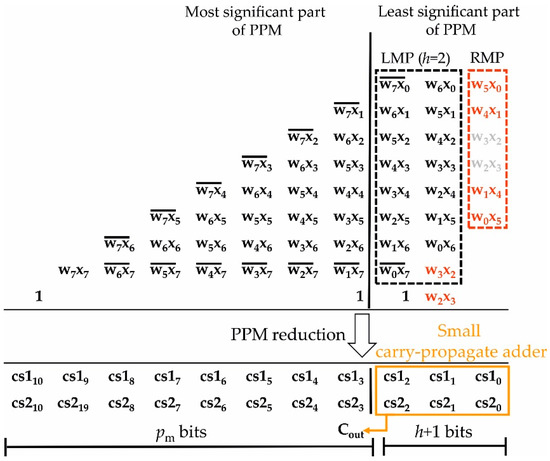
Figure 7.
Fixed-width multiplier with the output expressed in carry-save format. The small carry-propagate adder processes the h + 1 LSBs of cs1 and cs2 to compute Cout.
The truncation after the multiplication requires first to compute the output on pm + h + 1 bits and then to discard the h + 1 LSBs [34]. In this implementation, with the aim to further improve the performances, the output of the multiplier is kept in carry-save format (see the two rows cs1 and cs2 in the last stage of the multiplier) and a small carry-propagate adder is employed on the h + 1 less significant columns in order to compress the corresponding output terms (see the orange box in the figure) and to compute a single carry bit Cout. The carry Cout is added in the adder tree, which computes the filter output. This allows us to neglect all the carry-save bits in the first h + 1 columns, countered in the orange box of Figure 7. In this way, we avoid computing the product of each multiplier on pm + h + 1 bits (which would require a larger carry-propagate adder). In addition, the fixed-width approach also allows us to reduce the bit-width of the inputs of the adder tree.
2.4. Approximation with the Static Segment Method
2.4.1. Static Segment Method
The SSM technique proposed in [36] for the computation of the unsigned p × p multiplication is based on the employ of a pssm × pssm multiplier, with p/2 ≤ pssm < p, whose output is properly shifted in order to approximate the result of the p × p multiplication.
For the sake of simplicity, let us consider the case of the multiplication between two integer signals, a and b, with p = 8 bits. The example of Figure 8 shows an SSM multiplier with pssm = 5. As observable in Figure 8a, if the t = p − pssm MSBs of a are zero, we can perform the multiplication considering the remaining pssm LSBs. Conversely, if the MSBs are nonzero, we truncate the input a to its first pssm MSBs.
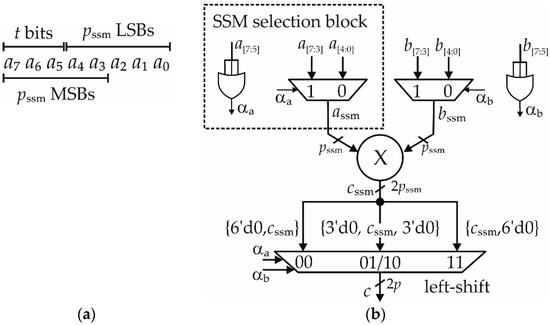
Figure 8.
(a) Working principle of the SSM approximation, and (b) scheme of the SSM multiplication.
To this aim, with reference to the input a, the SSM selection block of Figure 8b employs an OR-based circuit to study the bits a[p−1:pssm] (i.e., a[7:5] in the figure) and to compute the state flag αa, whereas the multiplexer selects the portions a[pssm−1:0] if αa = 0, or a[p−1:p-pssm] if αa = 1 (corresponding to a[4:0] and a[7:3] in the figure, respectively). Similarly, we can apply the same approximation to input b, as shown in Figure 8b.
In this way, the multiplier processes the outputs of the multiplexers, named assm and bssm in the figure, whose number of bits is pssm instead of p. At this point, a further multiplexer performs a left-shift operation to extend the product cssm on 2∙p bits. A shift of (p − pssm) positions is applied when either αa = 1 or αb = 1, and of 2∙(p − pssm) positions if both flags are high (shift of 3 and 6 positions in Figure 8b, respectively). On the contrary, no shift is used when αa and αb are low. In this way, the multiplier computes the exact output when both αa and αb are zero, whereas it approximates the result in the other cases.
2.4.2. Approximation with the Static Segment Method in the Feedback Section
A customized SSM technique is suitable for implementing the product |e(n − 1)|∙xsc(n − k − 1) in the MAC block. This specific application requires the multiplication between a small, unsigned value |e(n − 1)|, and the signed quantity xsc(n − k − 1). Since the error signal is close to zero at regime, the SSM selects only the LSBs of |e(n − 1)| without introducing any approximation on this signal. An error is in any way introduced when the MSBs of xsc(n − k − 1) are chosen. In this case, however, the approximation error has a small impact on regime performances, since by naming εxssm the module of approximation error on the input sample, εGssm the module of the approximation error on the gradient signal, and |essm(n − 1)| the absolute value of the error after the SSM selection, we have:
Therefore, the lower |essm(n − 1)| at regime, the lower the effects of the approximation on the learning algorithm.
Figure 9 shows the implementation of the learning section of the filter by using the SSM approach joined to the sign–magnitude technique introduced in Section 2.2. In the figure, the logic needed to introduce SSM approximation is highlighted in red. The SSM selection blocks (SSM sel. blocks in the figure) perform the segmentation of e(n) and of the input samples, as well as compute the flags αe, eflag, αx,k+1 and xflag,k+1, for k = 0, 1,…, N − 1, used by the SSM MAC blocks (named MSssm and highlighted in the red dashed rectangles). Please note that, in this topology, a single SSM sel. block of e(n) can be shared among all MSssm MACs and that the flags αe and eflag need to be delayed before to be sent in the learning section (see αeFF and eflagFF in the figure).
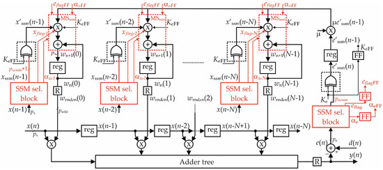
Figure 9.
Block diagram of the DLMS filter with static segmented MAC blocks in the learning section.
Figure 10a shows the segmentation applied to the error signal, whereas Figure 10b details the SSM sel. block. As shown in Figure 10a, we segment only the first p′e bits of e(n) since the MSB of the error epe−1 is always low after the XOR operation; therefore, we choose portions with pe,ssm ≥ p′e/2 bits.
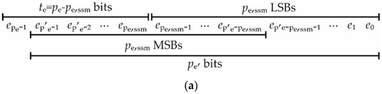
Figure 10.
(a) Segmentation scheme for the error signal and (b) related SSM selection block. (c) Segmentation scheme for the (k + 1)-th input sample and (d) related SSM selection block.
Being e(n) a signed signal, we need to select the pe,ssm LSBs when the error is small and positive, and when it is small in magnitude and negative. Otherwise, we approximate e(n) by means of its most significant part. To this aim, as shown in Figure 10b, the Signed Control Logic (SCL in the figure) studies the te = pe-pe,ssm MSBs of e(n) (corresponding to the portion e[pe−1:pe,ssm], see also Figure 10a) and their inverted version by means of two OR gates, and computes the state flag αe combining the output of the OR operations with an AND gate. In this way, the SCL is able to detect the condition in which the first te MSBs are low (i.e., e(n) small and positive) or are high (i.e., e(n) small in module and negative).
Afterwards, the multiplexer selects the segment e[pe,ssm−1:0] if αe = 0, or the segment e[p′e−1:p′e−pe,ssm] if αe = 1, whereas the resulting signal essm(n) is sent to the XOR bank. Please note that by segmenting the error signal before the XOR bank it is possible to reduce the XOR bank size.
In order to improve the accuracy of the SSM technique, in this paper, we employ a rounding operation (instead of the simple truncation used in [36]) to approximate the error signal when the MSBs are chosen (i.e., αe = 1). To that purpose, the most-significant bit of the discarded bits, that is bit e′p′e−pssm−1, is added to the segmented error signal when αe = 1. Please note that e′p′e−pssm−1, being one of the bits of the modulus of the error, is computed as the XOR between ep′e−pssm−1 and Ke (see Figure 10b). In this approach, by considering Equation (6) of the sign–magnitude technique, the segmented modulus error signal is written as:
In the case αe = 1, we can neglect the last term; therefore, we can approximate |essm(n)| as:
In conclusion, |essm(n)| can be written as:
where:
Figure 10b shows the implementation of Equations (18) and (19).
The segmentation scheme used for the input samples is represented in Figure 10c, whereas the related SSM sel. block, shown in Figure 10d, is based on the same considerations detailed in the case of the error signal. Please note that in this case, differently from the segmented output of the error signal, the segment that needs to be computed is a signed quantity; therefore, the selection needs to study the first tx = px − px,ssm + 1 MSBs of the input sample (see Figure 10c). In this way, when the less significant part is selected, the bit xpx,ssm−1, that belongs to the tx MSBs and is equal to the bits of x[px−1:px,ssm], acts as a sign bit for the segment and the suppression of the MSBs xpx−1 … xpx,ssm does not introduce any overflow condition. With reference to Figure 10d, the SCL logic studies the tx MSBs of x(n − k − 1) (corresponding to x[px−1:px,ssm−1]) and computes the (k + 1)-th state flag αx,k+1, whereas the multiplexer chooses between the portions x[px,ssm−1:0] and x[px−1:px−px,ssm], with px,ssm ≥ px/2.
Then, defining x′px−px,ssm−1 as the result of the XOR operation between xpx−px,ssm−1 and KeFF, we set the flag xflag,k+1 to x′px-px,ssm−1 if αx,k+1 = 1, or to KeFF otherwise; therefore, considering a LSB of weight 20, the sign-changed segmented input xsc,ssm(n − k − 1) is computed as:
where:
Again, the SSM selection improves the hardware complexity of the sign–magnitude DLMS since it allows to reduce the size of the XOR banks applied on the input samples.
By computing the registered version of (17) as:
and the gradient signal as:
we find the learning rule by substituting Equations (23) and (24) in (25):
where Wssm is a weight factor that describes the left-shift operation as follows:
Again, we specify that all the signals in (25) are supposed to be an integer for the sake of simplicity.
As a final remark, let us observe that in this paragraph, we have described the employ of SSM technique, highly customized for the feedback section of the filter. The SSM technique could also be employed to approximate the multipliers of the FIR section, but in this case less customized optimizations can be implemented, reducing the beneficial effects in terms of power dissipation and area. For this reason, we opted for the fixed-width approach previously described.
3. Results
3.1. Assessment of the Precision Performances
In order to quantify the precision of the proposed approach, we have considered a system identification problem. In this case, the DLMS filter has to track the impulse response of an unknown filter by observing its output d(n). The systems used for the identification can, in principle, be obtained by using different optimization and transformation filter design approaches (see, for example, [44,45]). In our case, for simplicity, we used the Matlab Filter Design and Analysis Tool with the following specifications:
- (i)
- Low pass, 38-th order, Equiripple FIR filter with pass band up to 0.4167π rad/sample and stop band with attenuation of 75 dB from 0.5417π rad/sample;
- (ii)
- Low pass, 7-th order, Infinite Impulse Response (IIR) filter with pass band up to 0.4167π rad/sample and stop band with attenuation of 60 dB from 0.75π rad/sample.
The impulse responses of the unknown filters are shown in Figure 11. In Figure 11b, the IIR impulse response is truncated to the first 50 elements, and the inset shows that the impulse response values asymptotically (for n → ∞) nullify. Please note that, similarly to other works (see for example [20]), we chose to consider two system identification cases, one (the FIR case) where the length of the impulse response corresponds to the length of the adaptive filter and another one (the IIR case) where the length of the impulse response, being infinite, is larger than the adaptive filter length.
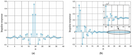
Figure 11.
Impulse response of (a) the FIR and of (b) the IIR unknown filters. The inset shows the tail of the IIR impulse response truncated on the first 50 elements.
We compute the steady-state MSE of the DLMS filter by observing the error signal of 500 independent trials. To this aim, we find the learning curve, representing the behavior of the MSE with respect to the time, by averaging the error signal of each simulation at each iteration n. Then, we find the regime MSE by averaging the last 10,000 samples of the learning curve. In these simulations, the input x(n) is white noise with uniform distribution in the range [−1,1).
In all the implementations, we quantize the input sample x(n) on px = 16 bits with LSBs of weight 2−15, as well as also the coefficients are represented with pw_fir = 16 bits with LSBs of weight 2−16. We suppose the desired output d(n) is expressed on 15 bits with resolution 2−13, whereas the error signals, which require guard bits to prevent any overflow during the transient phase of the learning, involve pe = 21 bits. Further, for e(n − 1), the LSB has weight 2−13. In addition, we remember that the condition p′e = 20 bits holds due to the relation p′e = pe − 1 presented in Section 2.2.
We choose the step size parameter as a power of two (i.e., µ = 2−6) with the aim to realize the product µ∙e(n − 1) by means of a hardwired shift. In this way, we avoid the introduction of a further multiplier in the adaptive filter. The coefficients at the output of the MAC block have pw = 37 bits with resolution 2−34. The number of taps used for the identification is N = 40.
We firstly present the analyses of the filters where only the feedback section is approximated.
In the fixed-width MAC blocks, we delete ptrunc = 14 LSBs of the updated coefficients wn+1(k) and preserve either h = 0 or h = 1 columns in the LMP of the PPM. In the following, we name these implementations FW14,0 and FW14,1, respectively.
In case of SSM approximation, we consider segments of either pe,ssm = 10 or pe,ssm = 11 bits for the xor-ed error, and portions of px,ssm = 8 bits for the input samples (implementations named SSM10,8 and SSM11,8, respectively). Please note that pe,ssm = 10 bits and px,ssm = 8 bits are the minimum bit-width for the segments essm(n) and xssm(n − k − 1) due to the conditions pe,ssm ≥ p′e/2 and px,ssm ≥ px/2.
For comparison, we have also implemented the DLMS filter proposed in [20,37,41] along with the standard version of the algorithm. The filter described in [20] involves the approximate Booth multiplier of [21] with 15 truncated columns in the FIR section, and adds up the rows of the PPM by means of a Wallace adder tree. In the learning section, the PPM is not pruned with the aim of preserving the steady-state MSE. The implementation of [37] exploits a modified version of the multipliers presented in [28] in which the authors compress the least significant partial products by means of OR gates. In addition, they suggest an exact compression only for the partial products obtained by means of NAND operation with the aim to reduce the approximation error. Further, the possibility to truncate some least significant columns is explored. In this comparison, we apply the approximate multipliers in the FIR section pruning pt = 11 and pt = 15 columns of the PPM. In [41], the learning section exploits the absolute value of the error signal for updating the coefficients. In addition, the authors approximate the input samples by lowering K or 2K LSBs at runtime as a function of the magnitude of the error, and design a multiplier able to combine the rounded inputs with the module of the error. For our analyses, we consider K = 2, 4, and 6.
Table 1 shows the regime performances of the filters.

Table 1.
Regime MSE of the proposed low-power implementations and of the state-of-the-art.
The proposed approximate implementations perform as the filters of [41] and exhibit a steady-state MSE practically unchanged with respect to the standard case. With the fixed-width approximation, the high precision performances are due to the compensation of the approximation error and to the suitable choice of the number of pruned LSBs ptrunc. As for the SSM approach, the approximation error due to the segmentation is strongly moderated by the error signal that is close to zero at regime (see also (14)). In particular, SSM10,8 and SSM11,8 are slightly more precise than FW14,0 and FW14,1. We also underline that the fixed-width implementation achieves remarkable results just with h = 0, i.e., with the minimum number of preserved columns in the PPM. Similarly, also the SSM approach achieves optimal results by involving multipliers with the minimum size (i.e., with pe,ssm = 10 and px,ssm = 8 in SSM10,8).
On the contrary, the approximations introduced in the cases [20,37] limit the steady-state MSE around −64 dB, and in the range −72/−76 dB, respectively. Figure 12 confirms the above considerations showing that the learning curves of the proposed filters superimpose to the exact one. In addition, also the convergence time is unchanged.
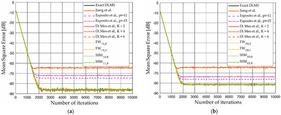
Figure 12.
Learning curves in the case of (a) FIR identification and (b) IIR identification with approximation in the feedback. In the figure, we report also the learning curves of the implementations Jiang et al. [20], Esposito et al. [37], and Di Meo et al. [41].
As the second step, we study the performances of the filter using the fixed-width technique for approximating the multipliers of the FIR section. Following (13), we choose ptrunc_fir = 12 in order to lower ε2fw of 18 dB with respect to ε2round, and preserve either h = 0 or h = 1 columns in the LMP. In these implementations, we also apply either one of the best approaches identified for the feedback section, that is, the SSM method (with pe,ssm = 10 and px,ssm = 8), or the fixed-with approach (with ptrunc = 14 and h = 0). We name these implementations FullFW14,0_fir12,0 and FullFW14,0_fir12,1 when the fixed-width approximation is considered both in FIR and feedback sections, and SSM10,8_FWfir12,0, and SSM10,8_FWfir12,1, when the SSM technique approximates the learning section and the fixed-width technique is used in the FIR section.
Table 2 collects the results and repeats the performances of [20,37,41] to simplify the reading, whereas Figure 13 represents the learning curves.
Table 2.
Regime MSE with approximation in the FIR section.
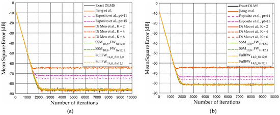
Figure 13.
Learning curves in the case of (a) FIR identification and (b) IIR identification with approximation in the learning and in the FIR sections. The learning curves of the implementations Jiang et al. [20], Esposito et al. [37], and Di Meo et al. [41] are reported for the sake of comparison.
The application of the fixed-width technique to the FIR section practically preserves the results obtained with the approximations in the learning, showing a steady-state MSE again very close to the standard case and [41]. Only a slight improvement is registered when h increases. Furthermore, as shown in Figure 13, also in this case, the proposed techniques preserve the convergence time.
It is worth noting that all the filters exhibit a slight degradation of the steady-state MSE when the IIR system is identified. This is due to the finite length of the impulse response that the DLMS filters exploit in comparison to the infinite length of the impulse response of the IIR system. We underline that our techniques offer unchanged steady-state MSE with respect to the standard DLMS also in this case; therefore, the proposed techniques allow preserving the quality of convergence regardless of the length of the unknown impulse response.
3.2. Assessment of the Electrical Performances
In order to analyze the hardware performances, we synthesize the proposed filters in TSMC 28 nm CMOS technology by means of Cadence Genus. For all the implementations, we used a physical synthesis flow with a clock period of 3.33 ns, and exploited post-synthesis simulations for the assessment of the power consumption. The path delays and the switching activity of the circuits were simulated by means of SDF and TCF format, respectively.
We analyze the performances of the filters FW14,0 and SSM10,8 when the approximation is applied only in the learning section since they offer the desired regime MSE with the minimum hardware overhead. At the same time, we assess the implementations SSM10,8_FWfir12,0, SSM10,8_FWfir12,1, FullFW14,0_fir12,0, and FullFW14,0_fir12,1 when also the FIR section is approximated.
Table 3 reports the obtained hardware performances of all considered filters. We can start by considering the proposed implementations where only the learning section of the filter is approximated. In this case, the implementation SSM10,8 reveals as the one providing the best area reduction (−16.5% with respect to the standard case) while the FW14,0 is the one achieving the best power dissipation reduction (up to −56.1% with respect to the standard case). In any way, the area occupation of both the SSM10,8 and FW14,0 improves compared to the filters of [41], in which the low-power technique involves a sensible increase in the area (around +24%). It is also worth highlighting that SSM10,8 results in any way in a remarkable power dissipation reduction (up to −52.4% with respect to the standard case) and that FW14,0 also provides a slight area improvement with respect to the standard implementation. We underline that the sign–magnitude technique requires additive logic for the computation of the error modulus and of the gradient signal. As a consequence, it tends to increase the area of the filter. Nevertheless, as also shown in the table, the proposed approximations are able to solve this point, allowing an improvement of the area performances with respect to the standard DLMS and [41].
Table 3.
Electrical performances.
The introduction of the fixed-width technique in the FIR section also seems to be beneficial, both in terms of area occupation and power dissipation. The implementation SSM10,8_FWfir12,0 results in the lowest area occupation (with the only exception of the low-precision implementation of Jiang et al. [20]) with an energy-saving that ranges between −54.7% and −59.1%. On the other hand, FullFW14,0_fir12,0 and FullFW14,0_fir12,1 exhibit a more modest area reduction (up to −6.3%) but achieve the best performances in terms of power with an improvement up to −64.1%. Indeed, the fixed-width technique, by not allowing the downsizing of the logic that handles the sign–magnitude method, results in more area being consumed with respect to SSM; therefore, the above comparison suggests choosing one of the implementations SSM10,8_FWfir12,0, and SSM10,8_FWfir12,1 if the area is the most important constraint, and to choose one of the FullFW14,0_fir12,0 and FullFW14,0_fir12,1 implementations if the power is the most critical design parameter.
We underline that [20] achieves the highest area reduction (−32.6%) and a remarkable power saving (−56.5% with IIR identification). Nevertheless, these performances involve a sensible worsening of the regime MSE, with a degradation up to 21.7 dB in the FIR identification case; therefore, the proposed implementations are the only ones able to achieve high regime precision with best performances in terms of power and area.
4. Discussion
As stated in the previous section, the proposed low-power implementations are able to ensure regime performances comparable to the standard case with hardware performances that result in a remarkable reduction in the area occupation and of the power dissipation. This is mainly due to the truncation of the PPM matrix in the fixed-width multipliers and to the reduced bit-width of the signals processed in the SSM approach.
The design [41] improves the energy dissipation at the cost of a high area overhead. This is mainly due to logic that approximates the input samples and to the XOR banks that implement the sign–magnitude technique. In addition, the sign–magnitude multipliers developed in [41] also require additional logic to process the rounded inputs, thus increasing the area occupation.
On the other hand, by using in the learning section the SSM technique developed in this paper, it is possible to practically halve the bit-width of the error and of the input samples and, accordingly, downsize all the XOR banks. At the same time, this approach also results in a remarkable reduction in the multiplier complexity of the learning section.
The fixed-width solution exhibits a lower area improvement since it preserves the bit-width of the input samples and of the error required for sign–magnitude logic; however, the PPM pruning in the feedback MACs is augmented by the additional switching activity reduction in the partial products due to sign–magnitude logic and the reduction in the size of the registers in the feedback section results in the best power dissipation performances by using this approach.
When the FIR section is also approximated, the fixed-width technique reduces the bit-width of the signals processed in the adder tree, thus allowing a further area and a power reduction. It is worth noting that, despite [20,37], our technique with fixed-width approximation in the FIR section is the only one able to improve the hardware performances without sacrificing the regime performance.
For a better assessment of the hardware performances, we plot the area reduction and the power saving of all the implementations with comparable MSE (in the range −85.9 dB/−86.2 dB for the FIR identification case, and in the range −81.3 dB/−81.5 dB for the IIR identification) in Figure 14. Implementations close to the bottom-left corner ensure higher power improvement along with the best area reduction. We underline that the designs [20,37], exhibit worse accuracy and, therefore, are excluded from the comparison. The standard DLMS filter is reported as a reference.
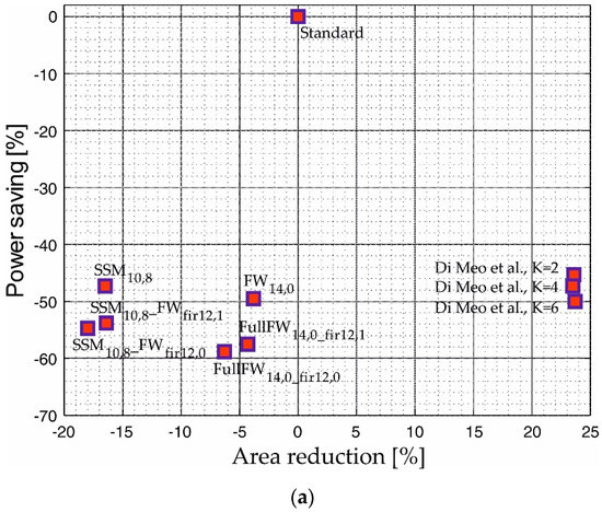
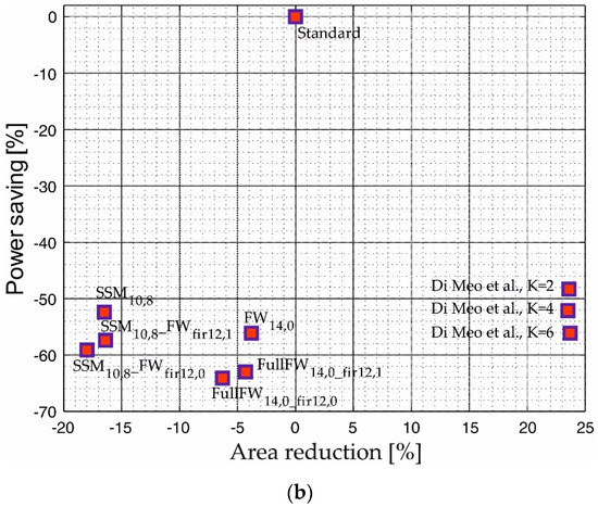
Figure 14.
Plot of the hardware features in terms of power saving and area reduction for the implementations with comparable regime MSE in the case of (a) FIR identification (MSE in the range −85.9 dB/−86.2 dB) and (b) IIR identification (MSE in the range −81.3 dB/−81.5 dB). The implementations by Di Meo et al. are related to the paper [41].
As shown, the filters of [41] are far from the optimal corner due to the high area overhead, whereas the proposed designs are able to improve both power and area. The figure shows again that the SSM approach allows best area results, whereas the fixed-width approximation performs better in terms of power. In addition, the implementations that approximate both the FIR and the learning sections are closer to the bottom-left corner, thus offering the best hardware improvements.
5. Conclusions
In this paper, we study the performances of the DLMS filter when approximate multipliers are used in the FIR and in the learning sections. The aim is to reduce the power consumption and the area while preserving the regime’s performance. We exploit a sign–magnitude representation for the error signal in order to improve the switching activity and the power consumption of the learning section and also approximate the arithmetic circuits of the filter for further optimizing the hardware performances. The first proposed techniques, applied to the learning section, involve either fixed-width or SSM approximate multipliers. The fixed-width technique provides to discard the less significant columns of the PPM, whereas the SSM approach reduces the number of bits of the inputs of the multipliers. The proposed methods are properly integrated with the sign–magnitude approach.
As the second step, we deal with the design of the FIR section by involving the fixed-width approximation and propose a suitable technique to properly integrate the bank of multipliers with the adder tree.
Results show that our proposals achieve steady-state performances practically unchanged with respect to the standard implementation considering the identification of both an FIR and an IIR unknown system. We underline that also in the IIR identification case, which is critical due to the infinite length of the unknown impulse response, the proposed filters are able to preserve the steady-state MSE with respect to the standard DLMS and [41]. In addition, the hardware performances improve, exhibiting remarkable power and area reductions with respect to [41]. When the learning section is approximated, the SSM technique allows the best area reduction (−16.5%), whereas the fixed-width approach ensures the highest power improvement (−56.1%). When the FIR section is also approximated, we register the best power saving with FullFW14,0_fir12,0 (−64.1%) and the best area reduction with SSM10,8_FWfir12,0 (−18.0%). Finally, from the analysis of Figure 14, we can conclude that the filters with approximation both in learning and in the FIR outperform the other implementations, offering the best area and power improvement.
Author Contributions
Conceptualization, G.D.M. and D.D.C.; methodology, G.D.M.; software, G.D.M.; validation, G.D.M. and D.D.C.; formal analysis, G.D.M. and D.D.C.; investigation, G.D.M. and D.D.C.; data curation, G.D.M.; writing—original draft preparation, G.D.M., D.D.C. and A.G.M.S.; writing—review and editing, D.D.C., N.P. and A.G.M.S.; visualization, G.D.M.; supervision, D.D.C., N.P. and A.G.M.S.; project administration, D.D.C. and A.G.M.S. All authors have read and agreed to the published version of the manuscript.
Funding
This research received no external funding.
Data Availability Statement
The MATLAB scripts and the Verilog modules are available on request to the corresponding author.
Conflicts of Interest
The authors declare no conflict of interest.
References
- Haykin, S. Adaptive Filter Theory; Prentice-Hall: Hobeken, NJ, USA, 2002. [Google Scholar]
- Rahman, M.Z.U.; Shaik, R.A.; Reddy, D.V.R.K. Adaptive noise removal in the ECG using the Block LMS algorithm. In Proceedings of the 2009 2nd International Conference on Adaptive Science & Technology (ICAST), Accra, Ghana, 14–16 December 2009; pp. 380–383. [Google Scholar] [CrossRef]
- Gupta, S.; Sharma, J.B. Estimation of respiratory rate from the ECG using instantaneous frequency tracking LMS algorithm. In Proceedings of the 2016 2nd International Conference on Advances in Computing, Communication, & Automation (ICACCA) (Fall), Bareilly, India, 30 September–1 November 2016; pp. 1–5. [Google Scholar] [CrossRef]
- Montanari, D.; Castellano, G.; Kargaran, E.; Pini, G.; Tijan, S.; De Caro, D.; Strollo, A.G.M.; Manstretta, D.; Castello, R. An FDD Wireless Diversity Receiver With Transmitter Leakage Cancellation in Transmit and Receive Bands. IEEE J. Solid-State Circuits 2018, 53, 1945–1959. [Google Scholar] [CrossRef]
- Colieri, S.; Ergen, M.; Puri, A.; Bahai, A. A study of channel estimation in OFDM systems. In Proceedings of the IEEE 56th Vehicular Technology Conference, Vancouver, BC, Canada, 24–28 September 2002; Volume 2, pp. 894–898. [Google Scholar] [CrossRef]
- Ting, L.K.; Woods, R.; Cowan, C.F.N. Virtex FPGA implementation of a pipelined adaptive LMS predictor for electronic support measures receivers. IEEE Trans. Very Large Scale Integr. (VLSI) Syst. 2005, 13, 86–95. [Google Scholar] [CrossRef]
- Albu, I.; Anghel, C.; Paleologu, C. Adaptive filtering in acoustic echo cancellation systems—A practical overview. In Proceedings of the 2017 9th International Conference on Electronics, Computers and Artificial Intelligence (ECAI), Piscataway, NJ, USA, 29 June–1 July 2017; pp. 1–6. [Google Scholar] [CrossRef]
- Yuan, Z.; Songtao, X. Application of new LMS adaptive filtering algorithm with variable step size in adaptive echo cancellation. In Proceedings of the 2017 IEEE 17th International Conference on Communication Technology (ICCT), Chengdu, China, 27–30 October 2017; pp. 1715–1719. [Google Scholar] [CrossRef]
- Tingchan, W.; Benjangkaprasert, C.; Sangaroon, O. Performance comparison of adaptive algorithms for multiple echo cancellation in telephone network. In Proceedings of the 2007 International Conference on Control, Automation and Systems, Seoul, Korea, 17–20 October 2007; pp. 789–792. [Google Scholar] [CrossRef]
- Meher, P.K.; Park, S.Y. Critical-Path Analysis and Low-Complexity Implementation of the LMS Adaptive Algorithm. IEEE Trans. Circuits Syst. I Regul. Pap. 2014, 61, 778–788. [Google Scholar] [CrossRef]
- Meyer, M.D.; Agrawal, D.P. A modular pipelined implementation of a delayed LMS transversal adaptive filter. In Proceedings of the 1990 IEEE International Symposium on Circuits and Systems (ISCAS), New Orleans, LA, USA, 1–3 May 1990; Volume 3, pp. 1943–1946. [Google Scholar] [CrossRef]
- Meher, P.K.; Park, S.Y. Area-Delay-Power Efficient Fixed-Point LMS Adaptive Filter With Low Adaptation-Delay. IEEE Trans. Very Large Scale Integr. (VLSI) Syst. 2014, 22, 362–371. [Google Scholar] [CrossRef]
- Long, G.; Ling, F.; Proakis, J.G. The LMS algorithm with delayed coefficient adaptation. IEEE Trans. Acoust. Speech Signal Process. 1989, 37, 1397–1405. [Google Scholar] [CrossRef]
- Mahfuz, E.; Wang, C.; Ahmad, M.O. A high-throughput DLMS adaptive algorithm. In Proceedings of the 2005 IEEE International Symposium on Circuits and Systems (ISCAS), Kobe, Japan, 23–26 May 2005; Volume 4, pp. 3753–3756. [Google Scholar] [CrossRef]
- Meher, P.K.; Maheshwari, M. A high-speed FIR adaptive filter architecture using a modified delayed LMS algorithm. In Proceedings of the 2011 IEEE International Symposium of Circuits and Systems (ISCAS), Piscataway, NJ, USA, 15–18 May 2011; pp. 121–124. [Google Scholar] [CrossRef]
- Liu, M.; Wang, M. An Efficient Architecture for the Modified DLMS Algorithm Using CIC Filters. In Proceedings of the 2018 Eighth International Conference on Instrumentation & Measurement, Computer, Communication and Control (IMCCC), Harbin, China, 19–21 July 2018; pp. 304–310. [Google Scholar] [CrossRef]
- Khan, M.T.; Shaik, R.A. Optimal Complexity Architectures for Pipelined Distributed Arithmetic-Based LMS Adaptive Filter. IEEE Trans. Circuits Syst. I Regul. Pap. 2019, 66, 630–642. [Google Scholar] [CrossRef]
- Guo, R.; DeBrunner, L.S. Two High-Performance Adaptive Filter Implementation Schemes Using Distributed Arithmetic. IEEE Trans. Circuits Syst. II Express Briefs 2011, 58, 600–604. [Google Scholar] [CrossRef]
- Vinitha, C.S.; Sharma, R.K. Area and Energy-efficient Approximate Distributive Arithmetic architecture for LMS Adaptive FIR Filter. In Proceedings of the 2020 International Conference for Emerging Technology (INCET), Belgaum, India, 5–7 June 2020; pp. 1–5. [Google Scholar] [CrossRef]
- Jiang, H.; Liu, L.; Jonker, P.P.; Elliott, D.G.; Lombardi, F.; Han, J. A High-Performance and Energy-Efficient FIR Adaptive Filter Using Approximate Distributed Arithmetic Circuits. IEEE Trans. Circuits Syst. I Regul. Pap. 2019, 66, 313–326. [Google Scholar] [CrossRef] [Green Version]
- Jiang, H.; Han, J.; Qiao, F.; Lombardi, F. Approximate Radix-8 Booth Multipliers for Low-Power and High-Performance Operation. IEEE Trans. Comput. 2016, 65, 2638–2644. [Google Scholar] [CrossRef]
- Han, J.; Orshansky, M. Approximate computing: An emerging paradigm for energy-efficient design. In Proceedings of the 2013 18th IEEE European Test Symposium (ETS), Avignon, France, 27–30 May 2013; pp. 1–6. [Google Scholar] [CrossRef]
- Chippa, V.K.; Chakradhar, S.T.; Roy, K.; Raghunathan, A. Analysis and characterization of inherent application resilience for approximate computing. In Proceedings of the 2013 50th ACM/EDAC/IEEE Design Automation Conference (DAC), New York, NY, USA, 29 May–7 June 2013; pp. 1–9. [Google Scholar] [CrossRef]
- Esposito, D.; Strollo, A.G.M.; Napoli, E.; De Caro, D.; Petra, N. Approximate Multipliers Based on New Approximate Compressors. IEEE Trans. Circuits Syst. I Regul. Pap. 2018, 65, 4169–4182. [Google Scholar] [CrossRef]
- Fritz, C.; Fam, A.T. Fast Binary Counters Based on Symmetric Stacking. IEEE Trans. Very Large Scale Integr. (VLSI) Syst. 2017, 25, 2971–2975. [Google Scholar] [CrossRef]
- Strollo, A.G.M.; Napoli, E.; de Caro, D.; Petra, N.; Meo, G.D. Comparison and Extension of Approximate 4-2 Compressors for Low-Power Approximate Multipliers. IEEE Trans. Circuits Syst. I Regul. Pap. 2020, 67, 3021–3034. [Google Scholar] [CrossRef]
- Strollo, A.G.M.; de Caro, D.; Napoli, E.; Petra, N.; di Meo, G. Low-Power Approximate Multiplier with Error Recovery using a New Approximate 4-2 Compressor. In Proceedings of the 2020 IEEE International Symposium on Circuits and Systems (ISCAS), Virtual, 10–21 October 2020; pp. 1–4. [Google Scholar] [CrossRef]
- Esposito, D.; Strollo, A.G.M.; Alioto, M. Low-power approximate MAC unit. In Proceedings of the 2017 13th Conference on Ph.D. Research in Microelectronics and Electronics (PRIME), Taormina, Italy, 12–15 June 2017; pp. 81–84. [Google Scholar] [CrossRef]
- Zervakis, G.; Tsoumanis, K.; Xydis, S.; Soudris, D.; Pekmestzi, K. Design-Efficient Approximate Multiplication Circuits Through Partial Product Perforation. IEEE Trans. Very Large Scale Integr. (VLSI) Syst. 2016, 24, 3105–3117. [Google Scholar] [CrossRef] [Green Version]
- Yang, Z.; Han, J.; Lombardi, F. Approximate compressors for error-resilient multiplier design. In Proceedings of the 2015 IEEE International Symposium on Defect and Fault Tolerance in VLSI and Nanotechnology Systems (DFTS), Amherst, MA, USA, 12–14 October 2015; pp. 183–186. [Google Scholar] [CrossRef]
- Jou, J.M.; Kuang, S.R.; der Chen, R. Design of low-error fixed-width multipliers for DSP applications. IEEE Trans. Circuits Syst. II Analog. Digit. Signal Process. 1999, 46, 836–842. [Google Scholar] [CrossRef] [Green Version]
- Kidambi, S.S.; El-Guibaly, F.; Antoniou, A. Area-efficient multipliers for digital signal processing applications. IEEE Trans. Circuits Syst. II Analog. Digit. Signal Process. 1996, 43, 90–95. [Google Scholar] [CrossRef]
- De Caro, D.; Petra, N.; Strollo, A.G.M.; Tessitore, F.; Napoli, E. Fixed-Width Multipliers and Multipliers-Accumulators with Min-Max Approximation Error. IEEE Trans. Circuits Syst. I Regul. Pap. 2013, 60, 2375–2388. [Google Scholar] [CrossRef]
- Petra, N.; de Caro, D.; Garofalo, V.; Napoli, E.; Strollo, A.G.M. Truncated Binary Multipliers with Variable Correction and Minimum Mean Square Error. IEEE Trans. Circuits Syst. I Regul. Pap. 2010, 57, 1312–1325. [Google Scholar] [CrossRef]
- Petra, N.; de Caro, D.; Garofalo, V.; Napoli, E.; Strollo, A.G.M. Design of Fixed-Width Multipliers with Linear Compensation Function. IEEE Trans. Circuits Syst. I Regul. Pap. 2011, 58, 947–960. [Google Scholar] [CrossRef]
- Narayanamoorthy, S.; Moghaddam, H.A.; Liu, Z.; Park, T.; Kim, N.S. Energy-Efficient Approximate Multiplication for Digital Signal Processing and Classification Applications. IEEE Trans. Very Large Scale Integr. (VLSI) Syst. 2015, 23, 1180–1184. [Google Scholar] [CrossRef]
- Esposito, D.; di Meo, G.; de Caro, D.; Petra, N.; Napoli, E.; Strollo, A.G.M. On the Use of Approximate Multipliers in LMS Adaptive Filters. In Proceedings of the 2018 IEEE International Symposium on Circuits and Systems (ISCAS), Florence, Italy, 27–30 May 2018; pp. 1–5. [Google Scholar] [CrossRef]
- Esposito, D.; De Caro, D.; Di Meo, G.; Napoli, E.; Strollo, A.G.M. Low-Power Hardware Implementation of Least-Mean-Square Adaptive Filters Using Approximate Arithmetic. Circuits Syst Signal Process. 2019, 38, 5606–5622. [Google Scholar] [CrossRef]
- Esposito, D.; di Meo, G.; de Caro, D.; Strollo, A.G.M.; Napoli, E. Quality-Scalable Approximate LMS Filter. In Proceedings of the 2018 25th IEEE International Conference on Electronics, Circuits and Systems (ICECS), Bordeaux, France, 9–12 December 2018; pp. 849–852. [Google Scholar] [CrossRef]
- Di Meo, G.; De Caro, D.; Napoli, E.; Petra, N.; Strollo, A.G.M. Variable-Rounded LMS Filter for Low-Power Applications. In Applications in Electronics Pervading Industry, Environment and Society; Lecture Notes in Electrical Engineering; Saponara, S., De Gloria, A., Eds.; Springer: Berlin/Heidelberg, Germany, 2020; Volume 627. [Google Scholar] [CrossRef]
- Meo, G.D.; de Caro, D.; Saggese, G.; Napoli, E.; Petra, N.; Strollo, A.G.M. A Novel Module-Sign Low-Power Implementation for the DLMS Adaptive Filter With Low Steady-State Error. IEEE Trans. Circuits Syst. I Regul. Pap. 2022, 69, 297–308. [Google Scholar] [CrossRef]
- Jakati, J.S.; Kuntoji, S.S. A Noise Reduction Method based on Modified LMS Algorithm of Real-time Speech Signals. WSEAS Trans. Syst. Control 2021, 16, 162–170. [Google Scholar] [CrossRef]
- Esposito, D.; Meo, G.D.; de Caro, D.; Napoli, E.; Petra, N.; Strollo, A.G.M. Stall-Aware Fixed-Point Implementation of LMS Filters. In Proceedings of the 2018 14th Conference on Ph.D. Research in Microelectronics and Electronics (PRIME), Prague, Czech Republic, 2–5 July 2018; pp. 169–172. [Google Scholar] [CrossRef]
- Stavrou, V.N.; Tsoulos, I.G.; Mastorakis, N.E. Transformations for FIR and IIR Filters’ Design. Symmetry 2021, 13, 533. [Google Scholar] [CrossRef]
- Tsoulos, I.G.; Stavrou, V.; Mastorakis, N.E.; Tsalikakis, D. GenConstraint: A programming tool for constraint optimization problems. SoftwareX 2019, 10, 100355. [Google Scholar] [CrossRef]
Publisher’s Note: MDPI stays neutral with regard to jurisdictional claims in published maps and institutional affiliations. |
© 2022 by the authors. Licensee MDPI, Basel, Switzerland. This article is an open access article distributed under the terms and conditions of the Creative Commons Attribution (CC BY) license (https://creativecommons.org/licenses/by/4.0/).