Assessment of Dual-Tree Complex Wavelet Transform to Improve SNR in Collaboration with Neuro-Fuzzy System for Heart-Sound Identification

Abstract

The research paper proposes a novel denoising method to improve the outcome of heart-sound (HS)-based heart-condition identification by applying the dual-tree complex wavelet transform (DTCWT) together with the adaptive neuro-fuzzy inference System (ANFIS) classifier. The method consists of three steps: first, preprocessing to eliminate 50 Hz noise; second, applying four successive levels of DTCWT to denoise and reconstruct the time-domain HS signal; third, to evaluate ANFIS on a total of 2735 HS recordings from an international dataset (PhysioNet Challenge 2016). The results show that the signal-to-noise ratio (SNR) with DTCWT was significantly improved (p < 0.001) as compared to original HS recordings. Quantitatively, there was an 11% to many decibel (dB)-fold increase in SNR after DTCWT, representing a significant improvement in denoising HS. In addition, the ANFIS, using six time-domain features, resulted in 55–86% precision, 51–98% recall, 53–86% f-score, and 54–86% MAcc compared to other attempts on the same dataset. Therefore, DTCWT is a successful technique in removing noise from biosignals such as HS recordings. The adaptive property of ANFIS exhibited capability in classifying HS recordings.

1. Introduction

Healthy cardiac valves (CV) are a sign of our overall health. The heart sounds (HS) measured by phonocardiograph (PCG) consist of 4 different sounds: S1, S2, S3, and S4 [1,2,3]. Various CV diseases can be detected from the heart sounds, mostly during S1 and S2, but the accuracy of such diagnoses largely depends on a cardiologist’s experience and expertise [2,3]. However, PCG is a complicated nonstationary signal in nonlinear low frequency, easily interfered with by surrounding signal sources [3,4].

HS recording, or PCG, is the only way to study and investigate the mechanical characteristics of the cardiac valvular system. In addition, some cardiovascular diseases can be followed in correlation to the PCG signals [5,6]. There is no golden standard of approach or a certain model that cardiologists can utilize to identify a cardiac disease relevant to valvular operations [2]. The main reason behind this fact is the variability of cardiac valvular disease. In other words, each valvular disease has its harmonic-frequency consistency that may lead to varying complexity and diversity in HS-signal appearance. For example, the frequency components of paradoxical splitting are arranged differently from aortic stenosis [2], while frequency ranges of murmurs differ from mitral regurgitation. To aid cardiologists in distinguishing healthy normal heart sounds (NrHS) from pathological heart conditions (HC), there have been numerous algorithms for automatic analysis and classification of HS [2]. The earliest attempt was in 1963 by Gerbarg et al. [1], who applied simple signal-processing steps (i.e., signal filters) on 1000 HS recordings. Since then, hundreds of attempts have been reported, but these applied advanced information technology methods, such as artificial neural networks (ANN) classifiers and advanced signal transforms, such as Fourier transform (FT) and wavelet transform (WT). Generally, the structure of recent HS classifiers consists of three main steps: a signal-denoising process; the extraction of signal features to discern HC from NrHS; and the application of a classifier such as ANN or deep learning (DL) (i.e., machine learning) [7]. The signal features are usually extracted from the time domain, wavelength, frequency domain, or morphological operations [8,9,10,11]. Many types of ANN and DL techniques have been applied on separate datasets with a range of good accuracies [12,13,14,15].

Although high accuracies in HS classification were recorded (e.g., exceeding 90% precision) in different studies, researchers argued the presence of certain limitations, including the following: possible HS distortion (i.e., noisy or incorrect HS acquisition), insufficient signal features, and a lack of training, all of which may decrease the percentage of classification accuracy. Another vital point is that some algorithms were experienced on clear HS signals, which were locally acquired with high quality by physicians. Therefore, two hypothesized questions have arisen in this issue: First, how do we unite the majority of research on one standard data set? Second, what conditions should be fulfilled in the proposed method/algorithm for HC detection? The second concern is less crucial than the first, because it can be handled by arguing for the researchers to explicitly describe any suggestive HS classifier.

Therefore, international HS databases were established in response to the first question. For example, in 2016, PhysioNet organized a dataset of HS recordings acquired from different HS-recording devices under different environmental conditions from different countries [16]. It is worth mentioning that the quality of HS recordings belonging to the PhysioNet database was extremely exposed to various types of noise. Therefore, it becomes the hardest HS dataset ever used to test any algorithm performance that the challenging research competitors may construct. Not only does the HS noise spectrum contain common types of noise (e.g., electromagnetic, power, body interference noise), but it also contains mistakes due to human errors (e.g., untrained medical staff) and external sound interferences.

The PhysioNet Challenge 2016 dataset, as a single data source, has allowed quantitative comparisons between different signal-processing techniques and artificial HS classifiers (i.e., algorithms) [4,17,18,19,20,21,22,23,24,25,26,27,28,29,30]. Several techniques and algorithms have been tested using the PhysioNet Challenge 2016 data set. This includes the AdaBoost classifier, Gram polynomials and probabilistic neural networks, the convolutional neural network (CNN), tensor techniques, ensemble feature-based feedforward neural networks (FNN), DropConnect neural networks (DCNN), LogitBoost, random forest, and cost-sensitive classifier [4,17,18,28,29,30]. The outcome indicated a range of classification accuracies from 75% to 92%.

Additionally, new reports evaluated the advanced information technology methods in the previous three years, yielding a range of 82% to 99% accuracy. For example, in Ref. [31], the deep CNN with block-stack style was efficiently employed with 12 feature maps to achieve an adequate HS classification of 93%, while on the same database, the CNN combined with deep-learning algorithms with 497 features was employed, resulting in 86.8% accuracy [32]. A slight modification on deep learning occurred in Ref. [33], where the 1-D CNN and feedforward neural network (F-NN) were used for the unsegmented HS signal. The continuous downsampling and application of the Savitzky–Golay filter imposed this method to produce an accuracy of 86%. Another attempt was performed in Ref. [34] with the combination of 1D-CNN and 1-D of local ternary pattern (1D-LTP) to obtain the features vector and complete the classification process with an accuracy of 91.7%. Deperlioglu et al. [35] suggested a different approach based on the resampled HS energies, which was later employed as a stacked autoencoder network (SAEN) to achieve an accuracy of 99.8%.

Some researchers found that the improved mel-frequency cepstrum coefficient (MFCC) is a suitable scheme to produce a set of features that may improve classification accuracy. For example, the MFCC combined with the convolutional recurrent neural networks was experienced to gain an accuracy of 98% [36]. In Ref. [37], MFCC is applied to form a new fixed-length feature vector called I-vector. Then, the reduced size of the I-vector by principle component analysis (PCA) is fed to the support vector machine (SVM) classifier to reach an accuracy of 97.34%. A new attempt to reduce the dimension of the feature was proposed by W. Han et al. [38]. The reduction process was associated with a classifier known as semi non-negative matrix factorization (SNMFNet), designed to make the low-dimension features of HS more valuable (accuracy 82%).

On the other hand, all proceeding reports employed a noise-elimination process (i.e., filtering) before applying the artificial classifier technique. They utilized one of three main techniques. These are either the application of HS’s noise filtering such as band-pass filtering to discard 50 Hz inference, the processing of HS’s frequency spectrum from the Fourier transform (FT), or the processing of the HS’s wavelet coefficients from the wavelet Transform (WT). The discrete wavelet transform (DWT) combined with the singular value decomposition (SVD) gained high performance in denoising HS signals. Unfortunately, it still (i.e., DWT) struggles with several disadvantages, such as high-level decomposition, Meyer mother-wavelet functions, and inadequate noise elimination primarily due to failure in the anti-aliasing and shifting invariance properties [39,40].

Therefore, in this paper, we test a new technique to denoise HS, utilizing the dual-tree complex wavelet transform (DTCWT) based on the PhysioNet Challenge 2016 dataset. The proposed algorithm runs offline, as the dataset was first downloaded and then processed as specified below. The DTCWT was modified from discrete wavelet transform (DWT) to overcome the drawbacks during both the sampling and reconstruction procedures, leading to the high signal-to-noise ratio (SNR). To the best of our knowledge, the DTCWT has not been tested on the PhysioNet database. Afterwards, six time-domain features were extracted from the HS signals and fed to the adaptive neuro-fuzzy inference System (ANFIS). This system has an adaptive property that could overcome a variety of sources for the same signal, which is the case for HS recordings in the PhysioNet database. It was recently successfully utilized on frequency-domain features [4], not time-domain features. Therefore, the objective of this paper is to test a new denoising technique (DTCWT) combined with an adaptive classifier (ANFIS) to manage HS time-domain signals from different devices and acquisition conditions. Our findings from 2735 HS signals indicate that the signal-to-noise ratio (SNR) was improved by DTCWT, suggesting this transform as a new technique to remove noise from biosignals. A set of only six time-domain features, fed to the ANFIS classifier, was able to recognize normal from abnormal HS signals, which are acquired from different sources.

2. Materials and Methods

The PhysioNet Challenge 2016 is an international open-access dataset of HS signals acquired from different locations worldwide, including nonclinical and clinical health facilities, using different medical recording instruments (available on the website https://physionet.org/content/challenge-2016/1.0.0/, accessed on 1 March 2021). The PhysioNet Challenge 2016 dataset has been implemented to develop robust algorithms aimed to deal with very noisy heart-sound signals [16]. All recorded data are aggregated as normal or pathological (abnormal) samples and portioned into five unbalanced recording classes (from A to E) each containing NrHS and HC signals (as detailed in

Table 1. Dataset distribution.

Class	Sets	# Subjects	Abnormal HC	Normal HS
A	Training	313	218	95
	Test	78	54	24
B	Training	356	72	284
	Test	88	18	70
C + D	Training	50	28	22
	Test	12	7	5
E	Training	1472	121	1351
	Test	366	28	338
A, B, C, D, E	Training	2191	439	1752
	Test	544	107	437
Total HS Signals	2735

) [16]. The cardiac valve diseases were considered as pathological type. The achieved accuracy refers to a statistical parameter called modified accuracy (Macc %). There are a total of 3153 HS in the dataset, with unevenly distributed HC severity among the classes [7]. In addition, each class was constructed to contain some external emergency noise such as uncontrolled environment voices [7,16]. The PhysioNet database was sourced from eight independent databases worldwide (more detailed information can be found in Ref. [16]).

(1)

MIT heart sounds database (MITHSDB) with 409 PCG recordings made at nine different recording positions and orientations from 121 subjects (age and gender unknown). Each subject contributed several recordings. The subjects were divided into:

(i)

normal control group: 117 recordings from 38 subjects;

(ii)

murmurs and mitral-valve prolapse (MVP): 134 recordings from 37 patients;

(iii)

118 benign murmurs recorded from 34 patients;

(iv)

aortic disease (AD): 17 recordings from 5 patients;

(v)

other miscellaneous pathological conditions (MPC).

(2)

Aalborg University heart sounds database (AADHSDB). The signals were recorded from 151 subjects (coronary angiography disease). Age and gender are unknown.

(3)

Aristotle University of Thessaloniki heart sounds database (AUTHHSDB). Forty-five subjects were enrolled with ages between 18 and 90 years.

(4)

Toosi Technology University heart sounds database (TUTHSDB): includes 16 patients with different types of cardiac-valve diseases (age and gender are unknown).

(5)

University of Haute Alsace heart sounds database (UHAHSDB). Nineteen normal subjects were recorded, with ages between 18 and 40 years; instead, the abnormal recordings were from 30 patients (10 females and 20 males) aged from 44 to 90 years.

(6)

Dalian University of Technology heart sounds database (DLUTHSDB). Subjects included 174 healthy volunteers (2 females and 172 males, aged from 4 to 35 years), and 335 patients (227 females and 108 males, aged from 10 to 88 years).

(7)

Shiraz University adult heart sounds database (SUAHSDB). The subjects included are 69 females and 43 males, aged from 16 to 88 years.

(8)

Skejby Sygehus Hospital heart sounds database (SSHHSDB): comprises 35 recordings from 12 normal subjects and 23 pathological patients with heart-valve defects (age and gender unavailable).

For our research work, we downloaded the HS recordings from all five classes in the dataset (Table 1) [16]. These HS recordings were divided into training and test sets using the 80–20% split protocol, as widely applied in ANN. We combined the class C data with class D due to their low numbers of HS signals to allow 80–20% ANN-split protocol. To meet the objectives of the paper, we discarded obvious distorted HS recordings that contained unusual external sounds using our experience as biomedical engineers; in conclusion, we extracted 2735 out of the 3153 HS recordings (in detail, 546 as pathological and 2189 as normal ones), approximately 87% of the entire dataset, as illustrated in Table 1. As the HS signal is periodic where S1 and S2 are repetitive, we assigned 5 s HS duration (i.e., all HS recording’s parts were included, S1, S2, S3, and S4, during the 5 s period) and sampled the signals at 2000 Hz, as per the PhysioNet specifications.

Figure 1 shows the block diagram of the proposed method; the HS recordings after the downloading were processed using the MATLAB library. The process begins by applying both the notch and Butterworth filters to the HS raw signal. Then, the resulting HS signal goes to the DTCWT for analysis and synthesis operations in order to denoise the HS recording, as explained below. To the best of our knowledge, the DTCWT, a tool that permits quantitative SNR analysis, has not been explored for the HS recordings in the PhysioNet Challenge 2016.

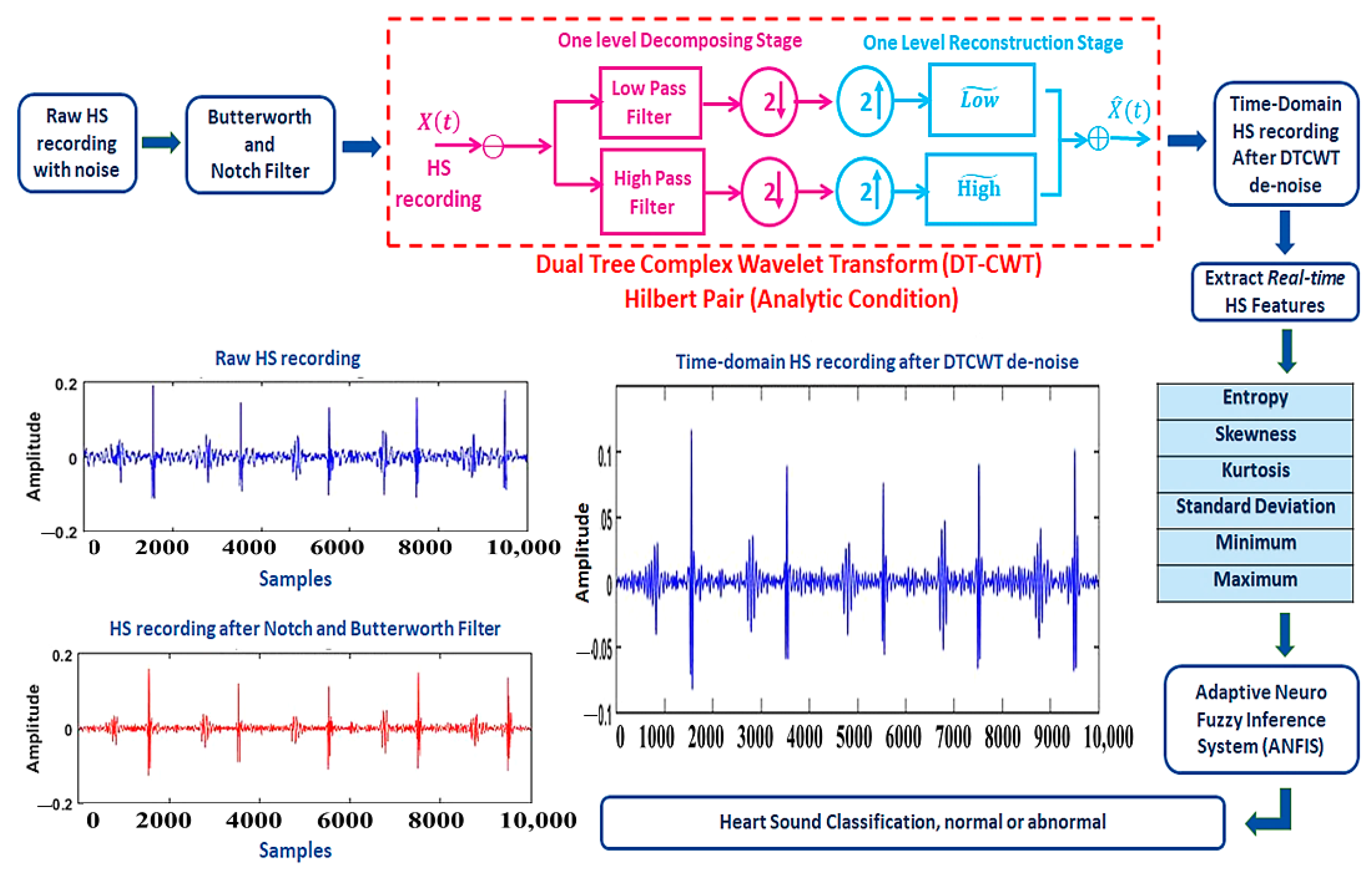
2.1. Preprocessing of HS Signal

Each raw HS signal was preprocessed using a notch filter to eliminate the primary 50–60 Hz noise. In this regard, the elimination of noise associated to the powerline (60 Hz) frequency was employed using an 4th-order infinite impulse response (IIR) notch filter with a 3 db stopband. We have used the Matlab function for band-stop IIR filter; the bandwidth of the notch filter is defined by the 59 to 61 Hz frequency interval with f_s equal to 2000 Hz, which provides attenuation up to 45 db and quality factor Q_F equal to 0.0333. Regarding the second-step filtration, the selected filter was a 4th-order Butterworth band-pass filter (BBF). Because of the minimal group delay, the finite impulse response (FIR) type was selected. The calculated lower and upper cut-off frequencies (f₁ and f₂) are 25 and 400 Hz, respectively. As with the first filtering step, the BBF was also implemented using the MATLAB library; the obtained Q_F (defined as F_center/(f₂ − f₁)) is equal to 0.2666 [41,42]. Figure 1 shows examples of an HS recording after applying the two signal- filtering steps.

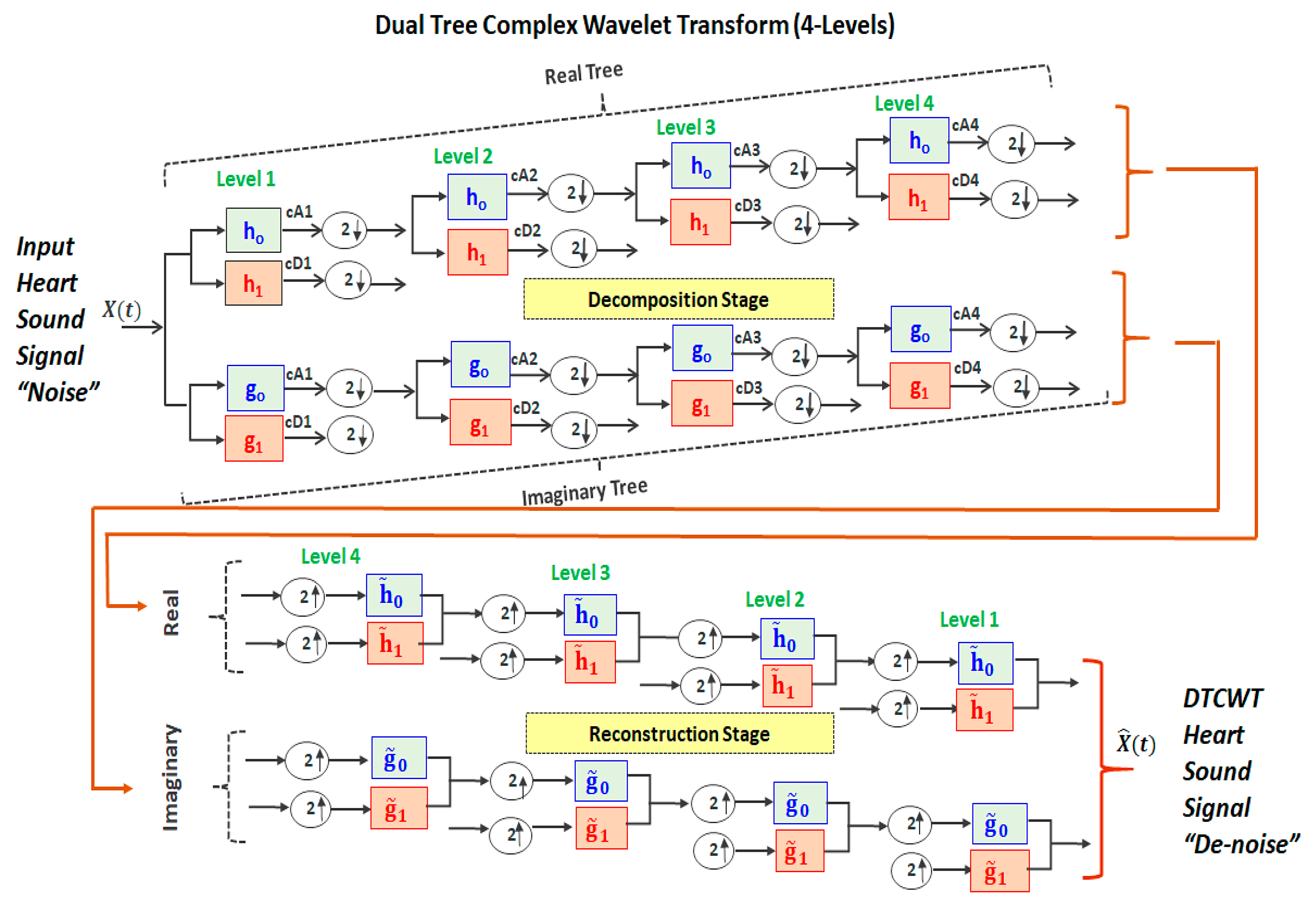
2.2. Dual-Tree Complex Wavelet Transform

Discrete wavelet transform (DWT), which was developed to aid signal analysis, suffers filtering difficulties during the sampling procedure, leading to inadequate noise elimination due to failure in the anti-aliasing and shifting invariance properties [39]. To overcome such limitations, DTCWT was developed to enhance noise abolition by DWT [41]. DTCWT includes sequential steps during the decomposition and reconstruction stages.

Figure 2 shows the typical structure of DTCWT, demonstrating both the decomposition and reconstruction stages. In the decomposition stage, the input signal X(t) (i.e., the HS recording) is fed to two signal-processing trees, known as dual trees (DT). The upper tree processes the real part of the signal, while the lower tree processes the imaginary one. Therefore, these two trees (real and imaginary) are called complex wavelet transform (CWT). Thus, this process is denoted as DT-CWT, or DTCWT. As shown in Figure 2, each tree can be considered as a filter-bank (FB) tree. The upper tree contains a low-pass filter (h₀) and high-pass filter (h₁) of the real part. Similarly, the lower tree contains the low and high pass filters, (g₀) and (g₁) of the imaginary part, respectively.

At level 1 during the decomposition process, the real part is divided into low-frequency (i.e., h₀) and high-frequency information (i.e., h₁). The low-frequency coefficient is called the approximate coefficient (cA1) and illustrated in Equation (1), while the high-frequency coefficient is called the detail coefficient (cD1) and is illustrated in Equation (3). This procedure is repeated in level 2, in which the previous low-frequency cA1 components are divided into low-cA2 and high-cD2 frequencies. The process is repeated until the end of level 4. Therefore, there are four approximate coefficients (cA1–cA4). Similarly, there are four detail coefficients (cD1–cD4) of the real constituents of the DWT of the real part. This process is identically applied to the imaginary part during the decomposition stage, resulting in four approximate coefficients (cA1–cA4) and four detail coefficients (cD1–cD4), but for the imaginary part of DWT. Mathematically, this would avoid the limitations of DWT, the anti-aliasing and shifting invariance [39]. Additionally, the real and imaginary frequencies’ components, which are presented in any signal (i.e., the HS recording in this paper), can be treated separately, eliminating the shift dependence during the DWT. Equations (1) and (3) explain the calculation of the approximate coefficient (cA) and detailed coefficient (cD).

It is important to note that at each decomposition level, the cA and cD sizes are repeatedly decreased by a factor of 2^d, which is the d-dimensional of the signal (i.e., the time and amplitude). The factor equal to 2 was selected because it provides the optimum DTCWT performance, as indicated in Ref. [39]. On the other hand, during the reconstruction process, as reported in Figure 2, a reverse procedure is applied on the real and imaginary parts to rebuild the signal successively (cA4–cA1 and cD4–cD1), yielding the progressive denoising of the signal. Thus, the output signal $\widehat{X}\left(t\right)$ is the denoised version of the input signal X(t), as demonstrated in Figure 2. The complete mathematical equations on DTCWT can be found in Ref. [39].

$$W_{\psi \left(n\right)}={{\displaystyle \sum }}_{k=0}^{N-1}d\left(k\right)\psi \left(n-k\right),$$

(1)

where $c{A}_{\psi \left(n\right)}$ is the Approximate coefficient, ψ(n) is the mother wavelet, and k is the shifting parameter. The “n” is a variable indicating the number of DTCWT levels “N” (i.e., n = 1, 2, 3, …, N). The “N” was set to 4 in this research work (i.e., 4 levels of DTCWT).

$$\psi \left(n\right)=\frac{1}{\sqrt{2j}}\psi \left(\frac{n-k2j}{2j}\right),$$

(2)

where j is the scaling parameter. The Equation of the details coefficients, which capture the high-frequency information, is reported below:

$$c{D}_{\phi \left(n\right)}={{\displaystyle \sum }}_{k=0}^{N-1}d\left(k\right)\phi \left(n-k\right),$$

(3)

where $c{A}_{\phi \left(n\right)}$ is the approximate coefficient, “n” and “N” are the same as in Equation (1), and φ(n) is the mother wavelet that is defined as

$$\phi \left(n\right)={\left(-1\right)}^n\psi \left(N-1-n\right),$$

(4)

Consequently, Figure 2 imitates successive filter banks during analysis-synthesis operations. It demonstrates that we first considered the real part of the decomposition operation. After four levels of decomposition and downsampling (1–1 up to 4–1 and 1–2 up to 4–2) ended, the second operation of signal reconstruction will start to recover the signal. It is often described as a mirror or reverse operation of signal synthesis. Again, the reconstruction process is applied on the real part from level 4 to 1 employing upsampling operations. In the end, these two signals will be averaged as one reconstructed output that is known as output $\widehat{X}\left(t\right)$.

Particularly, the DTCWT satisfies the well-known condition of Hilbert Analytic, which is illustrated in Figure 1 (denoted in dashed box), indicating that the scaling complex function and the wavelet complex function are isolated to generate the Hilbert pair of separately low-pass and high-pass filters. This was applied four times in Figure 2 (DTCWT) for the real and imaginary components of the signal after DWT. In other words, DTCWT processes the real and imaginary parts separately, which is denoted as the “complex shift process”.

The best performance of the DTCWT design can be achieved as reported in Refs. [42,43,44], when the internal structure of FBs satisfies the following three conditions:

• Implementing a perfect reconstruction (PR) to make the reconstructed signal $\widehat{X}\left(t\right)$ identical to the original (input) signal X(t). This condition is achieved when the input signal’s noise is successively attenuated until the end of the number of decomposition levels. Then, the next process (mirror operation) successively synthesizes (i.e., reconstructs) the resulting signals after noise reduction.
• Implementing successive half-sample shifts (i.e., dividing the samples by factor of 2) of both the low-pass filters (h₀ and g₀) and high-pass filters (h₁ and g₁) on the real and imaginary parts (dual trees). This would avoid any disorder in satisfying the Hilbert pair condition.
• Implement an equal-sample shift to have the same range of frequencies through all the CTDWT levels during the decomposition and reconstruction stages.

According to the Hilbert pair conditions, the net result is that DTCWT would solve DWT’s drawbacks by permitting q-shift (i.e., successive equal shifts) and anti-aliasing during the analysis and synthesis processes. Subsequently, the SNR of the signal, which is the HS signal in this paper, is expected to improve, thus allowing more precise time-domain feature extraction. In Ref. [45], an example is presented on how DTCWT can solve the DWT limitations. The result of biosignal decomposition into the scale (a4) and four detail coefficients (d1–d4) after applying DTCWT is reported, as well as the spectrum plot for each coefficient. It is clear that the only original frequency components are left on the output; no other components appear because of the successful decomposition with the downsampler and perfect reconstruction with the upsampler. This confirms that DTCWT is effectively reliable against frequency aliasing. Also in Ref. [45] it was demonstrated that the shift invariant’s ability in DTCWT in comparison with DWT. DTCWT has a similarity of delay instead of shocks and disorder of frequency rearrangement in the DWT. In the DWT, a small shift in signal or frequency may cause new changes in the output. However, DTCWT exhibits the ability to avoid the shift invariance. It is also possible to plot signals in the time domain during the preprocessing and signal-conditioning steps. However, in the wavelet domain, especially when dealing with signal decomposition into different levels using complex wavelet or discrete wavelet transform, it is restricted to sample scaling more than time scaling, based on the function and documentation related to Matlab and MathWorks software. Secondly, for the high-resolution presentation of DTCWT and DWT, the subsignal (decomposed level) is preferred to be plotted by samples rather than time (seconds).

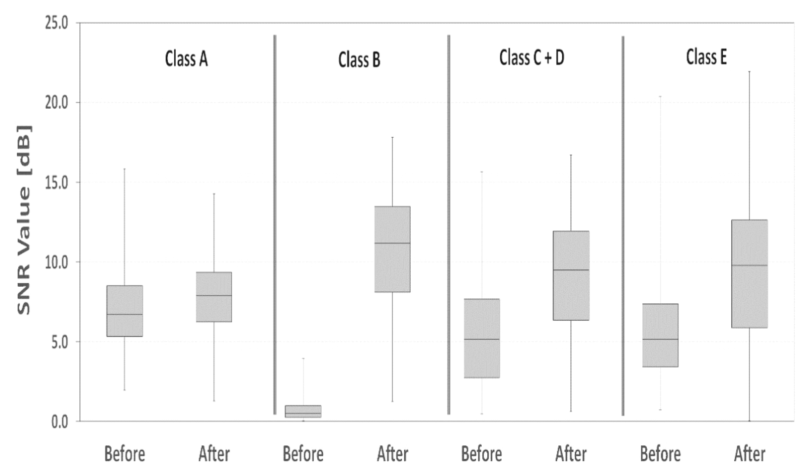
2.3. SNR Calculations

The HS signals are poorly recorded and frequently contain many types of ambient noises, such as electronic circuit noise and noises derived from the interface between electrodes and skin [7]. The SNR can be estimated in different ways [46,47,48]. In this article, the SNR was calculated to assess the DTCWT’s robustness in improving the HS recordings in the PhysioNet database. The used Equation (5) measures the accumulative residual noise.

$$\mathrm{SNR}=\frac{\overline{S_{ni}^2}}{\overline{R_{ni}^2}}$$

(5)

where $\overline{S_{ni}^2}$ is the mean square noise of the analyzed heart signal (HS), and $\overline{R_{ni}^2}$ is the mean square residual noise, which can be calculated as:

$$Rni=Sni-DS$$

(6)

where DS is the denoised HS. The residual noise was converted to decibels (dB) using Equation (7).

$${\mathrm{SNR}}_{\mathrm{dB}}=10{ \ast \log }_{10}\left(\mathrm{SNR}\right)$$

(7)

Then, the SNR percentage difference (SNR%) after DTCWT was calculated by Equation (8):

$$\mathrm{SNR}\%=\frac{\overline{SNRa} - \overline{SNRb}}{\overline{SNRb}}$$

(8)

where $\overline{SNRa}$ is the SNR mean after the DTCWT, and $\overline{SNRb}$ is the SNR mean before DTCWT.

2.4. Feature Extractions

From the time domain of the HS recordings after DTCWT, we extracted a set of six features, including the entropy, skewness, kurtosis, standard deviation (STDev), minimum (Min), and maximum (Max) (Figure 1). These features were calculated on the training NrHS and HC signals after applying DTCWT. Then, they were normalized between 0 and 1 using Equation (9) before being fed to the neural network.

$${\overrightarrow{\mathrm{F}}}_{\mathrm{j},\mathrm{normalized}}=({\overrightarrow{\mathrm{F}}}_{\mathrm{j}}-{\mathrm{F}}_{\mathrm{j},\min })/\left({\mathrm{F}}_{\mathrm{j},\max }-{\mathrm{F}}_{\mathrm{j},\min }\right)$$

(9)

where ${\overrightarrow{\mathrm{F}}}_{\mathrm{j}}$ and ${\overrightarrow{\mathrm{F}}}_{\mathrm{j},\mathrm{normalized}}$ are the original and normalized j-th feature values, respectively; ${\mathrm{F}}_{\mathrm{j},\min }$ and ${\mathrm{F}}_{\mathrm{j},\max }$ are the minimum and the maximum of the j-th feature values calculated for all 2735 samples, respectively. In other words, the j-th feature (j = 1 to 6) for n samples (n = 1 to 2735) was normalized between 0 and 1 values. Thus, the classification process, described in the following section, should not be affected by different magnitudes of HS signal.

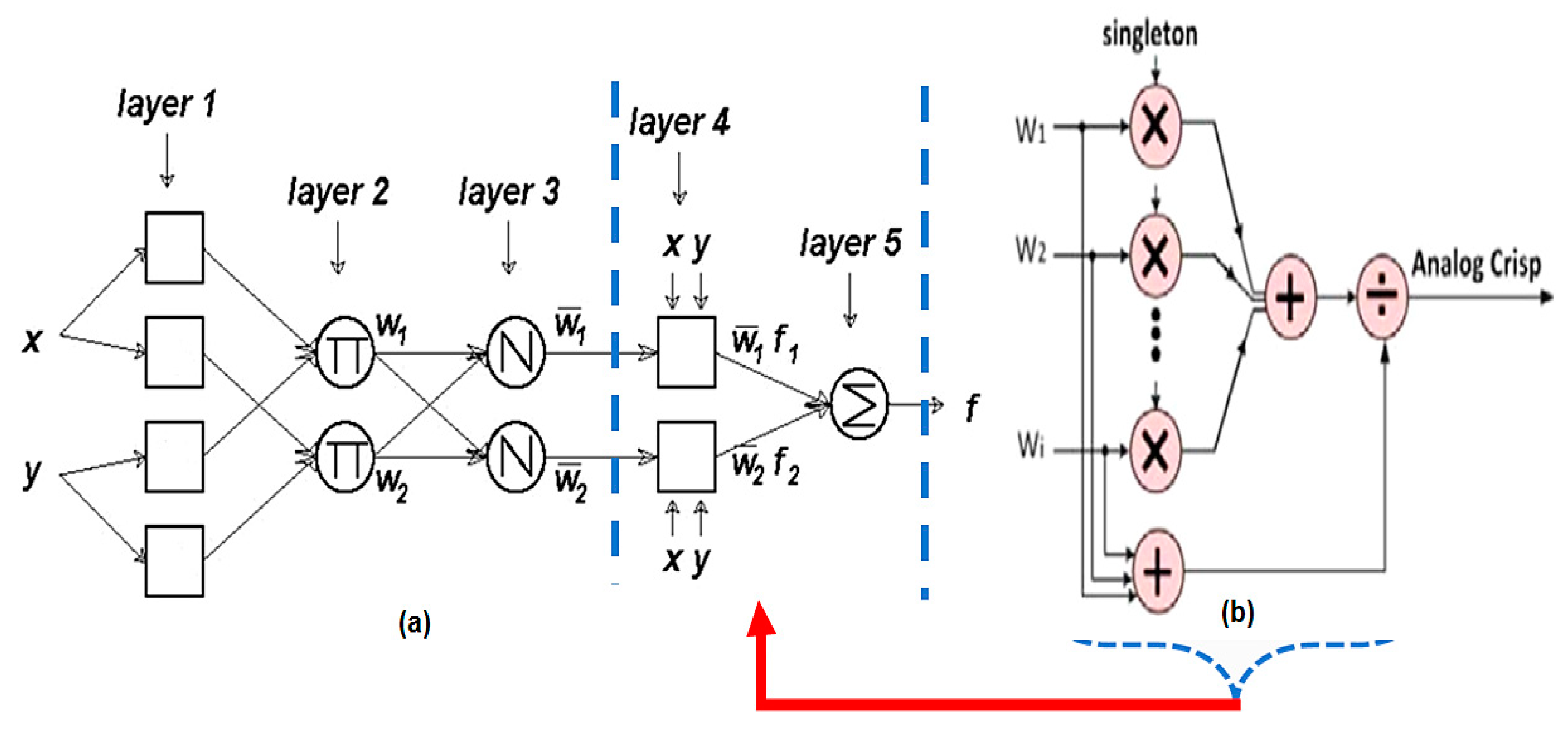
2.5. Adaptive Neuro-Fuzzy Inference System (ANFIS)

ANFIS is a machine-learning (ML)-based classifier algorithm. It is a rule-based method originally developed by Jang [48]. ANFIS has the ability of ANN ML that exploits a fuzzy inference system to deduce decisions by a fuzzy-logic method that takes into account the membership degree of input–output variables [48]. The ANFIS architecture has two fuzzy “if-then” rules based on the Sugeno model. The connection between the inputs and the Sugeno fuzzy output is fulfilled through five layers of nodes, as shown in Figure 3a: the fuzzy layer, product layer (Π), normalized layer (N), defuzzy layer, and total output layer, respectively. Layers 2 and 3 are adaptive with flexibility (i.e., fuzzy), while the other three layers (layers 1, 4, and 5) are fixed. The inputs (the six HS time-domain features) are distributed in the first layer based on their degree of membership into two groups and fed to layer 2. In layers 2 and 3, the “fuzzy” intersection and normalization are generated by implementing “fuzzy” weights, w1 and w2. Layer 4 is the defuzzy stage; the defuzzification unit is responsible for converting the input variables (fuzzy output of the inference engine) to a crisp using membership functions analogous to the function used in the fuzzifier layer. There are four defuzzification logic types: centroid of area (COA), weighted-average method (WAM), mean of maximum (MOM), and smallest of maximum (SOM) [48]. In this work, the WAM type was employed (as shown in Figure 3b), represented by Equation (10):

$$\mathrm{WAM}=\frac{{{\displaystyle \sum }}_{i=1}^n\left(W_i{S}_i\right)}{{{\displaystyle \sum }}_{i=1}^n\left(W_i\right)}$$

(10)

where W_i is the i’th output of the inference engine, S_i is the i’th singleton, and n is the number of singletons (in

Table 2. The training parameters of the ANFIS software.

TYPE	SUGENO
FIS and Method	Prod
FIS or Method	Probor
FIS defuzzification Method	Wtaver is the weighted average performance of all rule outputs (i.e., WAM).
FIS implication Method	Prod
FIS aggregation Method	Sum
FIS inputs	1 × 6 fisvar
FIS Outputs	1 × 1 fisvar
FIS rules	6 fis rule
Epoch number	200
Range of influence	0.5
FIS Creates a Sugeno FIS	Fis.Name = “sug41”

, the FIS defuzzification method). To end, layer 5 is the ANFIS classification decision’s output layer. ANFIS is available in the MATLAB instruction library.

The ANFIS structure should first rehearsed using the training set to derive the optimum performance before it is evaluated on the test sets. Therefore, we applied the ANFIS to all HS recordings in the training sets in Table 1. The ANFIS training optimum parameters are illustrated in Table 2. After that, the ANFIS was evaluated on the test sets in Table 1.

The training-test procedure was repeated five times (i.e., 5-fold cross-validation procedure) by repeating the 20–80% ANN protocol five times to each class of the HS dataset (Table 1). This should lead to better ANFIS performance accuracy. Figure 4 shows an example of the ANFIS outputs on the test set on class A in Table 1. The blue color indicates HC signals, while the red indicates NrHS signals. The ANFIS output was set to either one if pathology was predicted, or two if pathology was not predicted. Finally, the ANFIS performances were assessed by calculating the F-score, precision (or sensitivity), and recall (or positive predictivity) using Equations (11)–(13), respectively. Additionally, the modified accuracy (MAcc) was calculated, which is the average of precision and recall rates (i.e., (precision+ recall)/2). In addition, we did not utilize the true negative (TN) cases because most heart-sound-classification methods emphasize detecting heart-valve conditions (true positive cases).

Precision = TP/(TP + FP)

(11)

Recall = TP/(TP + FN)

(12)

F-score = 2*Precision*Recall/[Precision + Recall]

(13)

where:

-

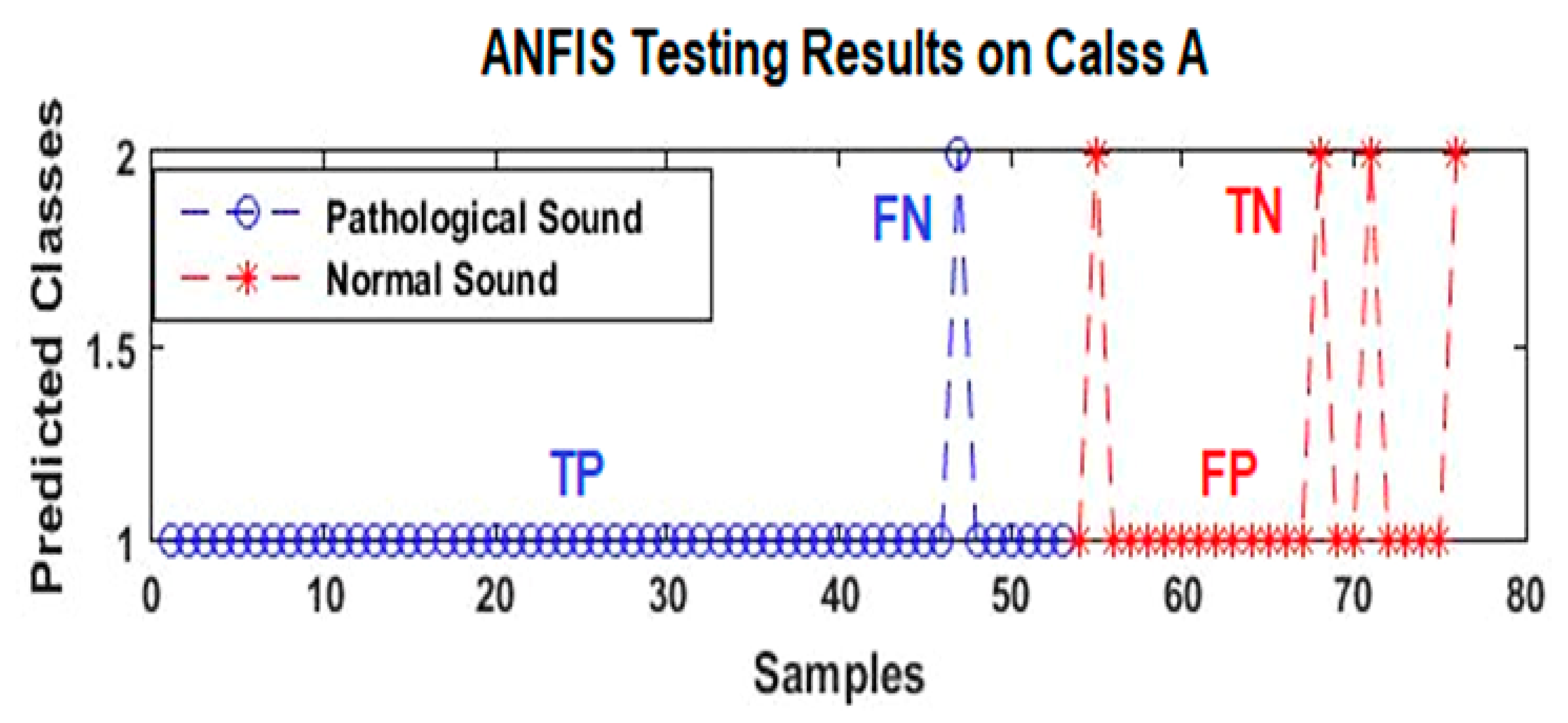
TP: true positive represents the HC-pathological samples detected correctly;

-

FP: false positive represents the NrHS-normal samples detected as abnormal;

-

TN: true negative represents the NrHS-normal samples detected correctly;

-

FN: false negative represents the HC samples detected as NrHS.

3. Results

For each HS signal (normal or abnormal), the SNR was calculated twice before and after applying DTCWT.

Table 3. The SNR measurements before and after DTCWT for all HS recordings in the dataset.

Dataset (before and after DTCWT)		Average SNR [dB]	SNR Standard Deviation [dB]	SNR Percentage Difference [dB]	Statistical Significance p-Value
Class A	Before	7.1	2.4	+0.11	<0.001
	After	7.9	2.4
Class B	Before	0.7	0.6	+13.96	<0.001
	After	10.8	3.5
Class C + D	Before	5.6	3.7	+0.58	<0.001
	After	8.9	4.0
Class E	Before	5.6	3.0	+0.65	<0.001
	After	9.3	4.8

shows the average (AVG) and standard deviation (STDev) of SNR measurements on each class in the data set. It also shows the SNR percentage difference calculated from Equation (4) and statistical difference by z-test between SNR measurements. The AVG and STDev values indicate that SNR was increased after applying DTCWT with statistical significance (p-value < 0.001). Figure 5 illustrates the boxplot of results in Table 3, demonstrating additional proof of the SNR improvement after applying DTCWT.

In the second experiment, we calculated the time-domain features for each HS signal after DTCWT, then the ANFIS classifier was trained and applied to each test set. The rate of recall, precision value, and F-score were reported for each class in the dataset. The MAcc, which is often used in recent literature, was also reported.

Table 4. ANFIS performance on the dataset.

Data Set	Precision	Recall	F-Score	MAcc [%]
Class A	0.73	0.98	0.84	85.5
Class C + D	0.86	0.87	0.86	86.0
Class B	0.55	0.89	0.68	72.0
Class E	0.56	0.51	0.53	53.5
Average (A, B, C, D, E)	0.68	0.81	0.74	74.5

shows that the average precision, recall, F-score, and MAcc were 0.68, 0.81, 0.74, and 75%, respectively. Meanwhile, Figure 5 shows the boxplot of SNR measurements on HS recordings for the five classes in the dataset (Table 1), indicating an SNR increment after applying DTCWT. Finally, we compared our findings with several previous findings with wavelet transform and other approaches applied on PhysioNet challenge 2016 (

Table 5. Literature samples on PhysioNet Challenge 2016 using wavelet transform.

Author	Methodology	# Features	Neural Network Classifier	# HS Samples	Accuracy MAcc%
C. Potes et al. [28]	Time and frequency-domain features	124	CNN	3240	86%
Whitaker, B. M. et al. [22]	Sparse coding	20	SVM	2153 *	86.5%
M. Tschannen et al. [26]	Wavelet deep convolutional neural network (CNN)	25	SVM	1277 *	81.2%
Goda et al. [49]	Wavelet envelope features	128	SVM	3000	81.2%
Langley et al. [50]	Wavelet Entropy	Wavelet entropy	Classification algorithm	400 *	77%
Kay E. et al. [18]	Hidden semi-Markov model	50	Fully connected, two-hidden-layer neural network trained by error backpropagation	All datasets excluding Class E *	74.8%
Grzegorczyk et al. [12]	Algorithm based on Hidden Markov Model.	48	Neural networks	3000	79%
Nilanon et al. [27]	Spectrogram	Many time windows	SVM, CNN, and logistic regression (LR)	About 3000	68–80%
M. N. Homsi et al. [51]	Nested ensemble of algorithms	131	Random forest, LogitBoost, and a cost-sensitive classifier	764 *	84.48%
This work	DTCWT	6	ANFIS	2735	74.5%
				Dataset excluding Classes B, E	86%

* Part of the 3153 HS recordings in the PhysioNet Challenge dataset were excluded.

).

4. Discussion

The results reported in Table 3 and Figure 5 show that there was an improvement in the average SNR values after applying the DTCWT for all classes in Table 1. The statistical significance (p < 0.001) reveals the capability of DTCWT in denoising HS recordings in PhysioNet 2016. Additionally, these results reveal inequality in the percentage of SNR improvement among the five different classes in the dataset. This result may suggest incoherent noise conditions during HS recordings, likely due to various instruments, diverse recording conditions, and/or potential human interferences. Therefore, the results, on the one hand, represent numerical proof that the different classes contain unequal noise conditions, making some HS recordings impracticable or incorrect. On the other hand, it shows that DTCWT can eliminate noise due to different types and levels of embedded noises.

Furthermore, Table 3 shows that class A has the lowest SNR percentage difference with no change in STDev after DTCWT, whereas classes B and E exhibit the largest SNR difference along with a large change in STDev after DTCWT. It suggests that class A exhibits the lowest level of embedded noise in the HS recordings compared to the other classes. Similarly, the combined C + D resulted in a nearly equal STDev, indicating the possible preservation of the HS signal while eliminating noise during the DTCWT. In contrast, after DTCWT, STDev increased by a few decibels for classes B and E, indicating the possible weakening of HS signals. The high SNR for the Class B dataset (as reported in Table 3) may be attributed to one or all of the following factors: the type of abnormal HS recordings (i.e., type of disease), the acquisition conditions, the type of environmental noise, and human errors. These factors were declared by the PhysioNet dataset organizer, who explicitly stated that the number of normal, abnormal, and distorted (i.e., occult) HS recordings was unequally distributed among the different classes in the Physionet database. They left it as a challenge and unseen to researchers. Thus, the Class B dataset probably contains more distorted HS recordings than other classes; in other words, the different SNR improvements reported in Table 3 derive from the unequal distribution of the type and severity of the added noise to the HS recordings. The DTCWT has shown the capability to detect these factors in the PhysioNet dataset, proving to be a successful denoising technique for biosignals. In addition, the obtained results shown in Figure 5 sustain the previous arguments that the order of the lowest to the highest number and severity of noisy HS recordings in the PhysioNet dataset is in the following order: Class A, C + D, E, and finally B. These findings are consistent with previous studies arguing that classes B and E contain the poorest quality of HS recordings [16,23]. Kay et al. [18] argued that Class E should be excluded from PhysioNet Challenge 2016 because it contains clinically nonpractical HS recordings. The same latter argument was claimed by Gjoreski et al. [7].

Analyzing the ANFIS-classifying performances in Table 4 shows that ANFIS outputs on classes B and E appeared to be unsatisfactory in terms of accuracy. The ANFIS classifier is a machine code that can be trained to provide optimal performance, so it is unlikely to be the reason. Therefore, the shortage in performance can be attributed to the quality of HS recordings, likely suggesting that classes B and E contained impractical HS signals, as claimed by references [12,18,27,28]. The potential solutions for this issue could be either to increase the number of input features to ANFIS classifier as in references [21,23,30,49] or to segment S1 and S2 portions from the five-second HS recordings, as in References [19,20,22,30].

Nonetheless, our ANFIS performed mathematical calculations to achieve 73–86% precision, 87–98% recall, 84–86% f-score, and approximately 86% MAcc (Table 3). This result was achieved on all the HS signals in classes A, C, and D, which presumably contained the correct S1–S2 segments, suggesting that ANFIS’s adaptive property with only six time-domain features performs well in classifying biosignals such as HS recordings. Our outcome is different from the previous findings [4] in many aspects. First, we tested DTCWT for denoising HS signals instead of the Fourier bispectrum. Second, we employed time-domain instead of frequency-domain features as inputs to ANFIS analysis. Third, we employed kurtosis and skewness as inputs to ANFIS. Since we applied the new method in Figure 1 on 2735 instead of 1738 signals, we consider our outcomes in this paper to be more reliable. Therefore, combining the results in this paper along with our previous study [4] rationalized the statement that the adaptive property in ANFIS with either time-domain or frequency-domain features performs well in classifying biosignals such as HS recordings.

When compared with previous attempts (Table 5), we found that DTCWT is a feasible solution to denoise HS signals. This finding has not been reported in literature before. Some previous studies excluded doubtful HS signals in designing satisfactory HS decision-support systems [4,18,22,26,42,51]. However, there were other attempts in which researchers included almost the entire 3153 PhysioNet datasets, so they had to implement a high number of input features—more than a hundred [27,28,49,51,52]. All these attempts yielded a range of MAcc values from 75% to 86%, which come close to results reported in this paper. Although our accuracy is lower than some of the previous outcomes, it is within the range of previous reports when impractical HS recordings are excluded, particularly classes B and E, as argued by references [7,12,18,26]. Finally, it is important to mention that this paper, in comparison to literature, quantitatively presented a significant SNR percentage difference after applying denoising, affirming that DTCWT can perform differently for different types and levels of embedded noises in PhysioNet 2016 [53].

It is worth mentioning that Chirplet transform (CT) has been strongly used for biomedical signal enhancement. It’s a combination of the application of short-time Fourier transform (STFT) with wavelet transform found by Mann et al. [54]. In the few reported works, CT was employed to heart-sound recordings provided by the Github database (Not PhysioNet 2016) [55]. The pristine quality of the Github database was the most significant factor in increasing the classification accuracy regardless of the machine learning used [56,57]. On the other hand, in CT, wavelet functions do not contain any complex relationships or specifications, the same as DTCWT (minimum anti-aliasing and shift-invariance) [58]. Thus, if CT is applied to the poor quality of PhysioNet datasets, the accuracy may not exceed 88% (or 86 ± 5%). This prediction is induced based on the previously reported works in Table 5.

It is noteworthy that the performance of DTCWT and ANFIS may be affected by several parameters, one of which is the Butterworth filter cutoff frequencies. However, we speculate that any marginal change in the cutoff frequency would only make a marginal change in performance [41]. The other parameters likely affecting the performance are the cA and cD, the amplitude, and detail coefficients in DTCWT, respectively [39]. A follow-up prospective research of those two parameters may further improve the DTCWT reconstruction of the HS signal, followed by an improvement in ANFIS performance. Finally, the number of decomposition and reconstruction levels in DTCWT in Figure 2 could also have an impact.

In conclusion, this research work aimed to develop a method to distinguish pathological heart sounds from normal ones; precisely, to be tested on datasets from PhysioNet. Considering the recorded signals’ very poor quality, ANFIS demonstrates a stable and reliable performance in data classifications without influencing the overfitting attitude. However, the used datasets were tested on the same PhysioNet Challenge 2016, and many other machine-learning algorithms were involved. Therefore, a comparison analysis is provided in Table 5.

5. Conclusions

In this research study, a new approach for HS classification was developed utilizing DTCWT combined with ANFIS. The new approach was evaluated on the PhysioNet challenge 2016 dataset. The data were organized and divided into different groups (A, B, C, D, and E).

The DTCWT successfully recorded a gain of several decibels in SNR, attributed to the processing of the real and imaginary frequency components separately. After the noise elimination, ANFIS achieved a competitive classification accuracy (average value of 75%), utilizing six time-domain features on all HS recordings in the PhysioNet database. This achievement occurred due to the high SNR performance and impact of blank filters (down- and upsampling) during the decomposition and reconstruction operations. In addition, the successful selection of the extracted features was an obvious clean factor in increasing the classifier progress (ANFIS) to achieve various accuracies (53–86%) depending on the dataset’s quality. Nevertheless, if non-clinically accepted HS recordings were excluded, as in reports [10,16,17,20,24,48,50], the proposed approach with the capability of DTCWT and ANFIS could achieve 86% precision, 98% recall, and 86% accuracy, suggesting that DTCWT and ANFIS are successful tools. In conclusion, DTCWT has demonstrated three remarkable advantages and strengths. First, it guarantees high SNR gain by applying four levels of decomposition and reconstruction. Second, it can be applied with db4 instead of using db10 and Meyer mother-wavelet functions. Third, it can overcome DWT’s drawbacks, avoiding anti-aliasing and shift invariance during the signal denoising process.

References

1. Gerbarg, D.S.; Taranta, A.; Spagnuolo, M.; Hofler, J.J. Computer analysis of phonocardiograms. Prog. Cardiovasc. Dis. 1963, 5, 393–405. [Google Scholar] [CrossRef]
2. Dwivedi, A.K.; Imtiaz, S.A.; Rodriguez-Villegas, E. Algorithms for automatic analysis and classification of heart sounds—A systematic review. IEEE Access 2019, 7, 8316–8345. [Google Scholar] [CrossRef]
3. Shub, C. Echocardiography or auscultation? How to evaluate systolic murmurs. Can. Fam. Physician 2003, 49, 163–167. [Google Scholar] [PubMed]
4. Al-Naami, B.; Fraihat, H.; Gharaibeh, N.Y.; Al-Hinnawi, A.-R.M. A Framework classification of heart sound signals in physionet challenge 2016 using high order statistics and adaptive neuro-fuzzy inference system. IEEE Access 2020, 8, 224852–224859. [Google Scholar] [CrossRef]
5. De Fazio, R.; De Vittorio, M.; Visconti, P. Innovative IoT solutions and wearable sensing systems for monitoring human biophysical parameters: A review. Electronics 2021, 10, 1660. [Google Scholar] [CrossRef]
6. De Fazio, R.; Stabile, M.; De Vittorio, M.; Velázquez, R.; Visconti, P. An overview of wearable piezoresistive and inertial sensors for respiration rate monitoring. Electronics 2021, 10, 2178. [Google Scholar] [CrossRef]
7. Gjoreski, M.; Gradisek, A.; Budna, B.; Gams, M.; Poglajen, G. Machine learning and end-to-end deep learning for the detection of chronic heart failure from heart sounds. IEEE Access 2020, 8, 20313–20324. [Google Scholar] [CrossRef]
8. De Vos, J.P.; Blanckenberg, M.M. Automated pediatric cardiac auscultation. IEEE Trans. Biomed. Eng. 2007, 54, 244–252. [Google Scholar] [CrossRef] [PubMed] [Green Version]
9. Herzig, J.; Bickel, A.; Eitan, A.; Intrator, N. Monitoring cardiac stress using features extracted from s1 heart sounds. IEEE Trans. Biomed. Eng. 2015, 62, 1169–1178. [Google Scholar] [CrossRef] [PubMed]
10. Li, H.; Ren, Y.; Zhang, G.; Wang, R.; Cui, J.; Zhang, W. Detection and classification of abnormities of first heart sound using empirical wavelet transform. IEEE Access 2019, 7, 139643–139652. [Google Scholar] [CrossRef]
11. Schmidt, S.; Graebe, M.; Toft, E.; Struijk, J. No evidence of nonlinear or chaotic behavior of cardiovascular murmurs. Biomed. Signal Process. Control 2011, 6, 157–163. [Google Scholar] [CrossRef]
12. Grzegorczyk, I.; Solinski, M.; Lepek, M.; Perka, A.; Rosinski, J.; Rymko, J.; Stepien, K.; Gieraltowski, J. PCG Classification Using a Neural Network Approach. In Computing in Cardiology; IEEE Computer Society: Washington, DC, USA, 2016; Volume 43, pp. 1129–1132. [Google Scholar] [CrossRef]
13. Chauhan, S.; Wang, P.; Lim, C.S.; Anantharaman, V. A computer-aided MFCC-based HMM system for automatic auscultation. Comput. Biol. Med. 2008, 38, 221–233. [Google Scholar] [CrossRef] [PubMed]
14. Saraçoğlu, R. Hidden Markov model-based classification of heart valve disease with PCA for dimension reduction. Eng. Appl. Artif. Intell. 2012, 25, 1523–1528. [Google Scholar] [CrossRef]
15. Cheng, X.; Huang, J.; Li, Y.; Gui, G. Design and application of a laconic heart sound neural network. IEEE Access 2019, 7, 124417–124425. [Google Scholar] [CrossRef]
16. Liu, C.; Springer, D.; Li, Q.; Moody, B.; Juan, R.A.; Chorro, F.J.; Castells, F.; Roig, J.M.; Silva, I.; Johnson, A.E.W.; et al. An open access database for the evaluation of heart sound algorithms. Physiol. Meas. 2016, 37, 2181–2213. [Google Scholar] [CrossRef] [PubMed]
17. Beritelli, F.; Capizzi, G.; Sciuto, G.L.; Napoli, C.; Scaglione, F. Automatic heart activity diagnosis based on Gram polynomials and probabilistic neural networks. Biomed. Eng. Lett. 2017, 8, 77–85. [Google Scholar] [CrossRef] [PubMed]
18. Kay, E.; Agarwal, A. Drop Connected neural networks trained on time-frequency and inter-beat features for classifying heart sounds. Physiol. Meas. 2017, 38, 1645–1657. [Google Scholar] [CrossRef]
19. Liu, C.; Springer, D.; Clifford, G.D. Performance of an open-source heart sound segmentation algorithm on eight independent databases. Physiol. Meas. 2017, 38, 1730–1745. [Google Scholar] [CrossRef] [PubMed]
20. Homsi, M.N.; Warrick, P. Ensemble methods with outliers for phonocardiogram classification. Physiol. Meas. 2017, 38, 1631–1644. [Google Scholar] [CrossRef] [PubMed]
21. Rubin, J.; Abreu, R.; Ganguli, A.; Nelaturi, S.; Matei, I.; Sricharan, K. Classifying heart sound recordings using deep convolutional neural networks and mel: Frequency cepstral coefficients. In Proceedings of the 2016 Computing in Cardiology Conference (CinC), Vancouver, BC, Canada, 11–14 September 2016; IEEE: Piscataway, NJ, USA, 2016. [Google Scholar] [CrossRef]
22. Whitaker, B.M.; Suresha, P.B.; Liu, C.; Clifford, G.; Anderson, D.V. Combining sparse coding and time-domain features for heart sound classification. Physiol. Meas. 2017, 38, 1701–1713. [Google Scholar] [CrossRef]
23. Plesinger, F.; Viscor, I.; Halamek, J.; Jurco, J.; Jurak, P. Heart sounds analysis using probability assessment. Physiol. Meas. 2017, 38, 1685–1700. [Google Scholar] [CrossRef] [PubMed]
24. Vernekar, S.; Nair, S.; Vijayasenan, D.; Ranjan, R. A Novel approach for classification of normal/abnormal phonocardiogram recordings using temporal signal analysis and machine learning. In Proceedings of the 2016 Computing in Cardiology Conference (CinC), Vancouver, BC, Canada, 11–14 September 2016; IEEE: Piscataway, NJ, USA, 2016. [Google Scholar] [CrossRef]
25. Maknickas, V.; Maknickas, A. Recognition of normal-abnormal phonocardiographic signals using deep convolutional neural networks and mel-frequency spectral coefficients. Physiol. Meas. 2017, 38, 1671–1684. [Google Scholar] [CrossRef] [PubMed]
26. Tschannen, M.; Kramer, T.; Marti, G.; Heinzmann, M.; Wiatowski, T. Heart sound classification using deep structured features. In Proceedings of the 2016 Computing in Cardiology Conference (CinC), Vancouver, BC, Canada, 11–14 September 2016; IEEE: Piscataway, NJ, USA, 2016. [Google Scholar] [CrossRef]
27. Nilanon, T.; Purushotham, S.; Liu, Y. Normal/abnormal heart sound recordings classification using convolutional neural network. In Proceedings of the 2016 Computing in Cardiology Conference (CinC), Vancouver, BC, Canada, 11–14 September 2016. [Google Scholar] [CrossRef]
28. Potes, C.; Parvaneh, S.; Rahman, A.; Conroy, B. Ensemble of feature-based and deep learning-based classifiers for detection of abnormal heart sounds. In Proceedings of the 2016 Computing in Cardiology Conference (CinC), Vancouver, BC, Canada, 11–14 September 2016. [Google Scholar] [CrossRef]
29. Bobillo, I.D. A Tensor approach to heart sound classification. In Proceedings of the 2016 Computing in Cardiology Conference (CinC), Vancouver, BC, Canada, 11–14 September 2016. [Google Scholar] [CrossRef]
30. Zabihi, M.; Rad, A.B.; Kiranyaz, S.; Gabbouj, M.; Katsaggelos, A.K. Heart sound anomaly and quality detection using ensemble of neural networks without segmentation. In Proceedings of the 2016 Computing in Cardiology Conference (CinC), Vancouver, BC, Canada, 11–14 September 2016. [Google Scholar] [CrossRef]
31. Xiao, B.; Xu, Y.; Bi, X.; Zhang, J.; Ma, X. Heart sounds classification using a novel 1-D convolutional neural network with extremely low parameter consumption. Neurocomputing 2020, 392, 153–159. [Google Scholar] [CrossRef]
32. Li, F.; Tang, H.; Shang, S.; Mathiak, K.; Cong, F. Classification of heart sounds using convolutional neural network. Appl. Sci. 2020, 10, 3956. [Google Scholar] [CrossRef]
33. Krishnan, P.T.; Balasubramanian, P.; Umapathy, S. Automated heart sound classification system from unsegmented phonocardiogram (PCG) using deep neural network. Phys. Eng. Sci. Med. 2020, 43, 505–515. [Google Scholar] [CrossRef] [PubMed]
34. Er, M.B. Heart sounds classification using convolutional neural network with 1D-local binary pattern and 1D-local ternary pattern features. Appl. Acoust. 2021, 180, 108152. [Google Scholar] [CrossRef]
35. Deperlioglu, O. Heart sound classification with signal instant energy and stacked autoencoder network. Biomed. Signal Process. Control 2021, 64, 102211. [Google Scholar] [CrossRef]
36. Deng, M.; Meng, T.; Cao, J.; Wang, S.; Zhang, J.; Fan, H. Heart sound classification based on improved MFCC features and convolutional recurrent neural networks. Neural Netw. 2020, 130, 22–32. [Google Scholar] [CrossRef] [PubMed]
37. Adiban, M.; BabaAli, B.; Shehnepoor, S. Statistical feature embedding for heart sound classification. J. Electr. Eng. 2019, 70, 259–272. [Google Scholar] [CrossRef] [Green Version]
38. Han, W.; Xie, S.; Yang, Z.; Zhou, S.; Huang, H. Heart sound classification using the SNMFNet classifier. Physiol. Meas. 2019, 40, 105003. [Google Scholar] [CrossRef]
39. Selesnick, I.; Baraniuk, R.G.; Kingsbury, N.G. The dual-tree complex wavelet transform. IEEE Signal Process. Mag. 2005, 22, 123–151. [Google Scholar] [CrossRef] [Green Version]
40. Li, S.; Li, F.; Tang, S.; Xiong, W. A Review of Computer-aided heart sound detection techniques. BioMed Res. Int. 2020, 2020, 5846191. [Google Scholar] [CrossRef]
41. Bianchi, G. Electronic Filter Simulation & Design, 1st ed.; McGraw-Hill Professional: New York, NY, USA, 2007. [Google Scholar]
42. Al-Naami, B.; Owida, H.; Fraihat, H. Quantitative analysis signal-based approach using the dual tree complex wavelet transform for studying heart sound conditions. In Proceedings of the 2020 IEEE 5th Middle East and Africa Conference on Biomedical Engineering (MECBME), Amman, Jordan, 27–29 October 2020; pp. 1–4. [Google Scholar] [CrossRef]
43. Vermaak, H.; Nsengiyumva, P.; Luwes, N. Using the dual-tree complex wavelet transform for improved fabric defect detection. J. Sens. 2016, 2016, 9794723. [Google Scholar] [CrossRef] [Green Version]
44. Daubechies, I. Orthonormal bases of compactly supported wavelets. Commun. Pure Appl. Math. 1988, 41, 909–996. [Google Scholar] [CrossRef] [Green Version]
45. Wang, F.; Ji, Z. Application of the dual-tree complex wavelet transform in biomedical signal denoising. Bio-Med. Mater. Eng. 2014, 24, 109–115. [Google Scholar] [CrossRef] [PubMed]
46. Goodfellow, J.; Escalona, O.J.; Kodoth, V.; Manoharan, G. Efficacy of DWT denoising in the removal of power line interference and the effect on morphological distortion of underlying atrial fibrillatory waves in AF-ECG. In Proceedings of the World Congress on Medical Physics and Biomedical Engineering (IFMBE), Toronto, ON, Canada, 7–12 June 2015; Volume 51. [Google Scholar] [CrossRef]
47. Van Drongelen, W. Signal averaging. In Signal Processing for Neuroscientists; Elsevier BV: Amsterdam, The Netherlands, 2007; pp. 55–70. [Google Scholar]
48. Jang, J.-S.R. ANFIS: Adaptive-network-based fuzzy inference system. IEEE Trans. Syst. Man Cybern. 1993, 23, 665–685. [Google Scholar] [CrossRef]
49. Goda, M.A.; Hajas, P. Morphological determination of pathological pcg signals by time and frequency domain analysis. In Computing in Cardiology; IEEE Computer Society: Washington, DC, USA, 2016; pp. 1133–1136. [Google Scholar] [CrossRef]
50. Langley, P.; Murray, A. Abnormal Heart Sounds Detected from Short Duration Unsegmented Phonocardiograms by Wavelet Entropy. In Proceedings of the 2016 Computing in Cardiology Conference (CinC), Vancouver, BC, Canada, 11–14 September 2016; IEEE: Piscataway, NJ, USA, 2016. [Google Scholar] [CrossRef]
51. Homsi, M.N.; Medina, N.; Hernandez, M.; Quintero, N.; Perpinan, G.; Quintana, A.; Warrick, P. Automatic Heart Sound Recording Classification using a Nested Set of Ensemble Algorithms. In Proceedings of the 2016 Computing in Cardiology Conference (CinC), Vancouver, BC, Canada, 11–14 September 2016; IEEE: Piscataway, NJ, USA, 2016. [Google Scholar] [CrossRef]
52. Ghaffari, A.; Homaeinezhad, M.R.; Khazraee, M.; Daevaeiha, M.M. Segmentation of holter ECG waves via analysis of a discrete wavelet-derived multiple skewness-kurtosis based metric. Ann. Biomed. Eng. 2010, 38, 1497–1510. [Google Scholar] [CrossRef] [PubMed]
53. Singh-Miller, N.; Singh-Miller, N. Using Spectral Acoustic Features to Identify Abnormal Heart Sounds. In Computing in Cardiology; IEEE Computer Society: Washington, DC, USA, 2016; pp. 557–560. [Google Scholar] [CrossRef]
54. Mann, S.; Haykin, S. The chirplet transform: Physical considerations. IEEE Trans. Signal Process. 1995, 43, 2745–2761. [Google Scholar] [CrossRef] [Green Version]
55. Ghosh, S.K.; Ponnalagu, R.N.; Tripathy, R.K.; Acharya, U.R. Deep layer kernel sparse representation network for the detection of heart valve ailments from the time-frequency representation of PCG recordings. BioMed Res. Int. 2020, 2020, 8843963. [Google Scholar] [CrossRef]
56. Shuvo, S.B.; Ali, S.N.; Swapnil, S.I.; Al-Rakhami, M.S.; Gumaei, A. CardioXNet: A novel lightweight deep learning framework for cardiovascular disease classification using heart sound recordings. IEEE Access 2021, 9, 36955–36967. [Google Scholar] [CrossRef]
57. Popov, B.; Sierra, G.; Durand, L.-G.; Xu, J.; Pibarot, P.; Agarwal, R.; Lanzo, V. Automated extraction of aortic and pulmonary components of the second heart sound for the estimation of pulmonary artery pressure. In Proceedings of the 26th Annual International Conference of the IEEE Engineering in Medicine and Biology Society, San Francisco, CA, USA, 1–5 September 2004; IEEE: Piscataway, NJ, USA, 2007; Volume 1, pp. 921–924. [Google Scholar]
58. Djebbari, A.; Bereksi-Reguig, F.A. New Chirp-based wavelet for heart sounds time-frequency analysis. Int. J. Commun. Antenna Propag. 2011, 1, 92–102. [Google Scholar]
Figure 1. Block diagram of the proposed HS recordings’ denoising and ANN classifier.
Electronics 11 00938 g001
Figure 2. One-dimensional DTCWT illustrating the filter banks during both the decomposition and reconstruction stages. X(t) represents the input signal; cA1, cA2, cA3, and cA4 denote the approximate coefficients at level 1, level 2, level 3, and level 4, respectively; while cD1, cD2, cD3, and cD4 denote the detail coefficients at level 1, level 2, level 3, and level 4, respectively. The upper and lower trees show the real and imaginary parts of the X(t) signal processing. The average signal is presented as an output X ^ ( t ) .
Electronics 11 00938 g002
Figure 3. The five layers-based structure of the ANFIS (a) and the defuzzification WAM internal structure (b).
Electronics 11 00938 g003
Figure 4. ANFIS testing results for class A dataset.
Electronics 11 00938 g004
Figure 5. SNR measurements on all HS recordings on all classes before and after utilizing DTCWT.
Electronics 11 00938 g005