
Automatically Learning Formal Models from Autonomous Driving Software

 , , and
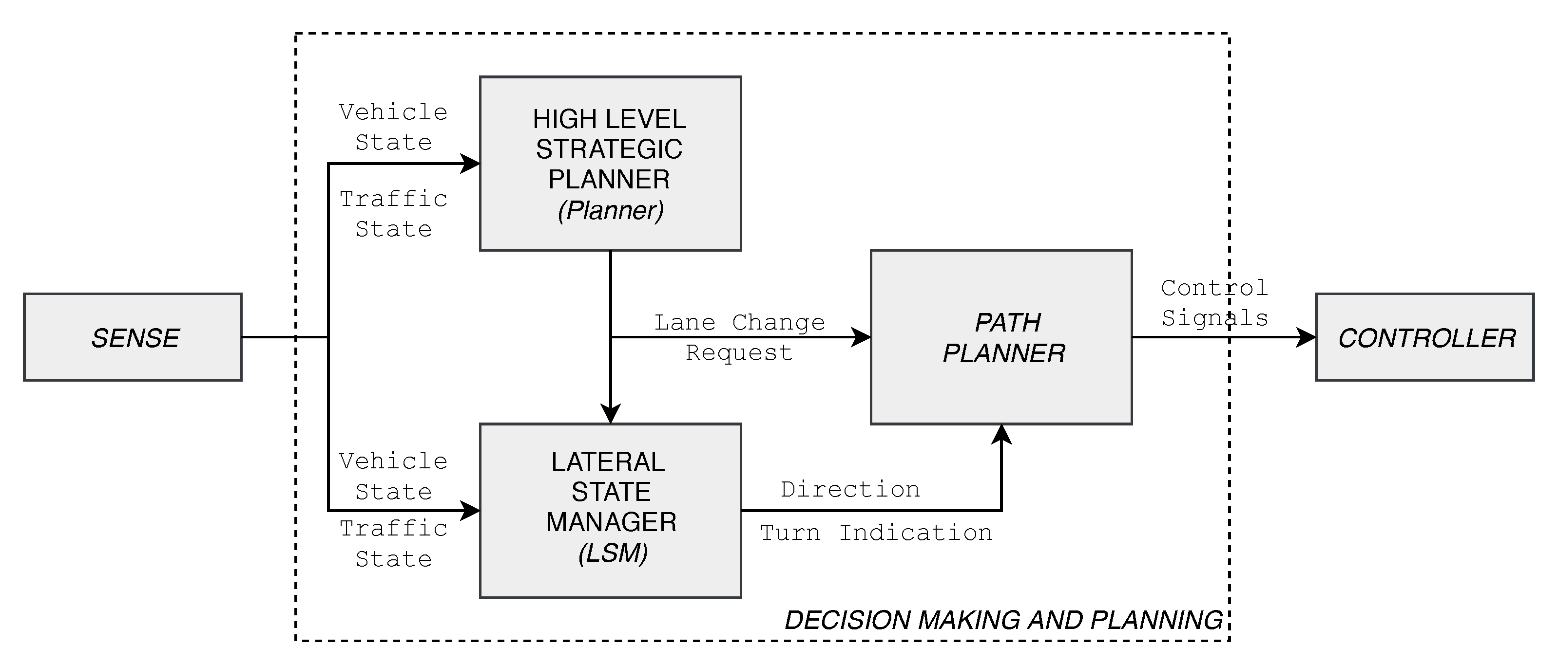
Abstract
:1. Introduction
- An evaluation on the practical applicability of to automatically learn a model of the LSM is presented based on experiments using LearnLib, an open-source automata learning framework [32], in addition to MIDES.
- Analysis of the learning outcome is performed by investigating optimizations that can potentially help improve the practical applicability of the learning algorithms.
- New insights on the approach of using automata learning to enable formal automotive software development is presented.
1.1. Related Work
2. System under Learning: The LSM
3. Preliminaries
- Q is the finite set of states;
- Σ is the alphabetof events;
- is the partial transition function;
- is the initial state;
- is the set of marked states.
- if there exists s.t. and
4. The Learning Algorithms
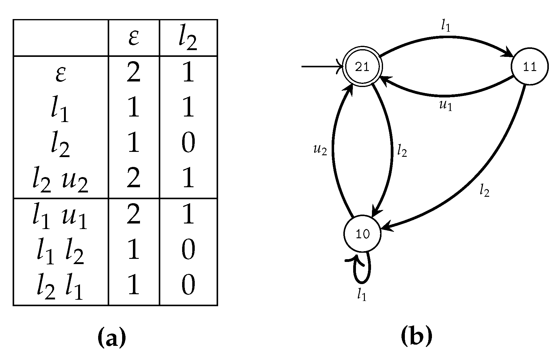
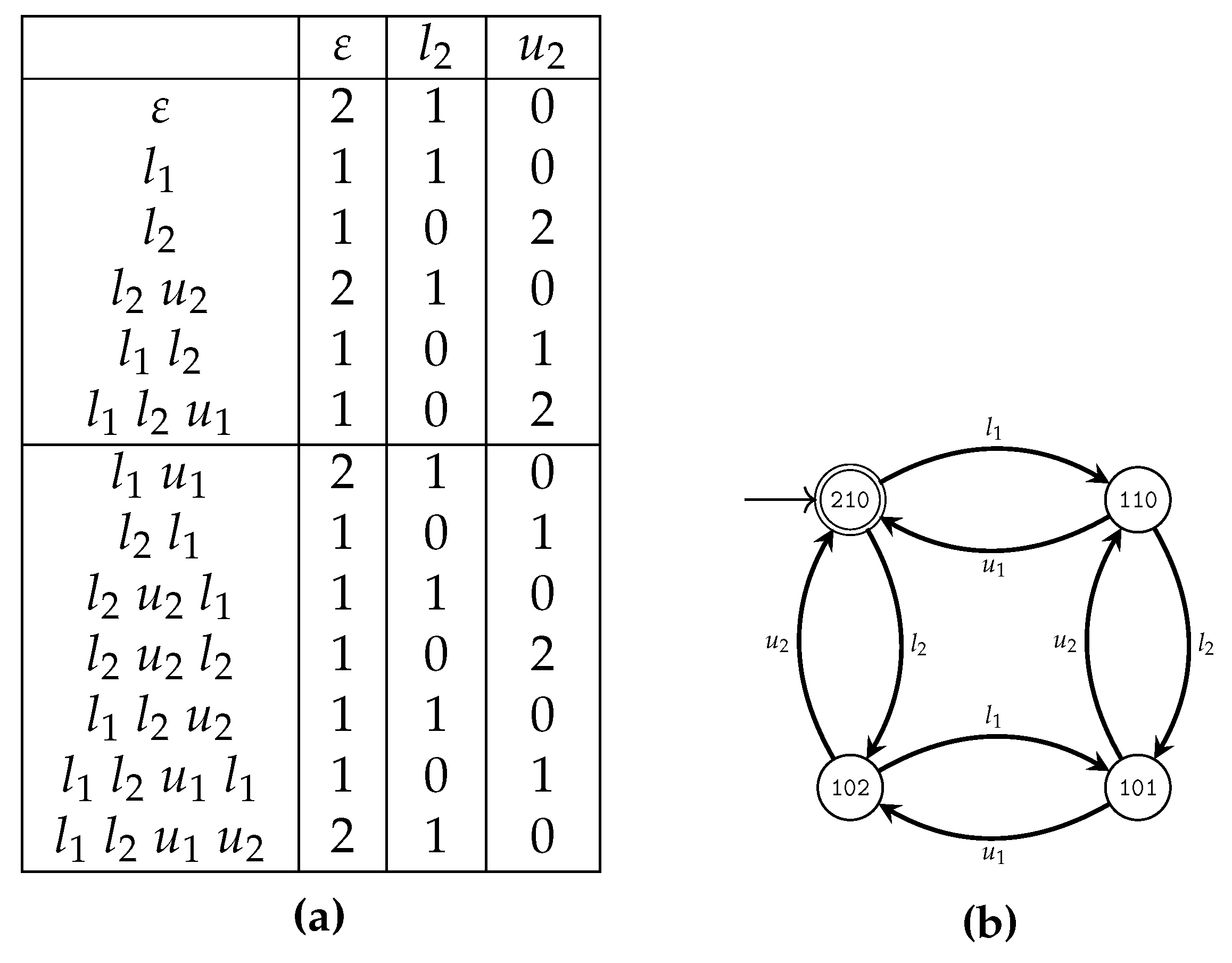
4.1. The Algorithm
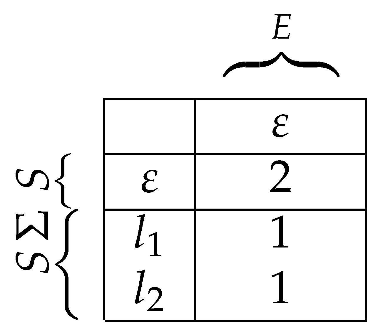
- Membership Queries:
- Given a string , a membership query for s returns 2 if the string can be executed by the SUL and takes the system (from the initial state) to a marked state. If the string can be executed, but does not reach a marked state, 1 is returned. Otherwise, 0 is returned. The membership query has the signature: , and for and :
- Equivalence Queries:
- Given a hypothesis automaton , an algorithm verifies if represents the language . If not, a counterexample must be provided, such that, either c is incorrectly generated (that is, but ), or incorrectly rejected (that is, but ) by . In this work, equivalence queries are performed using the W-method [53].Let have n states. Given a hypothesis , with states, the W-method creates test strings to iteratively extend the hypothesis until it has states.
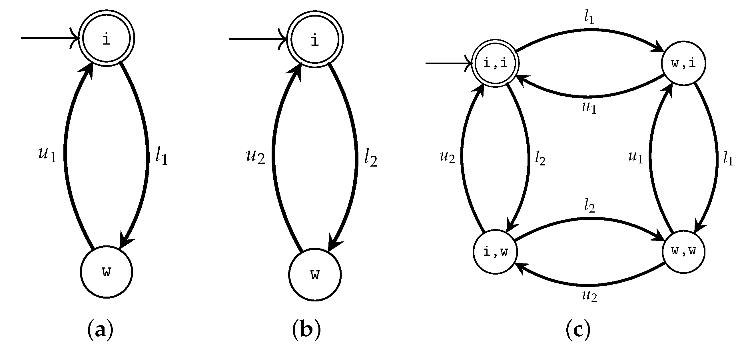
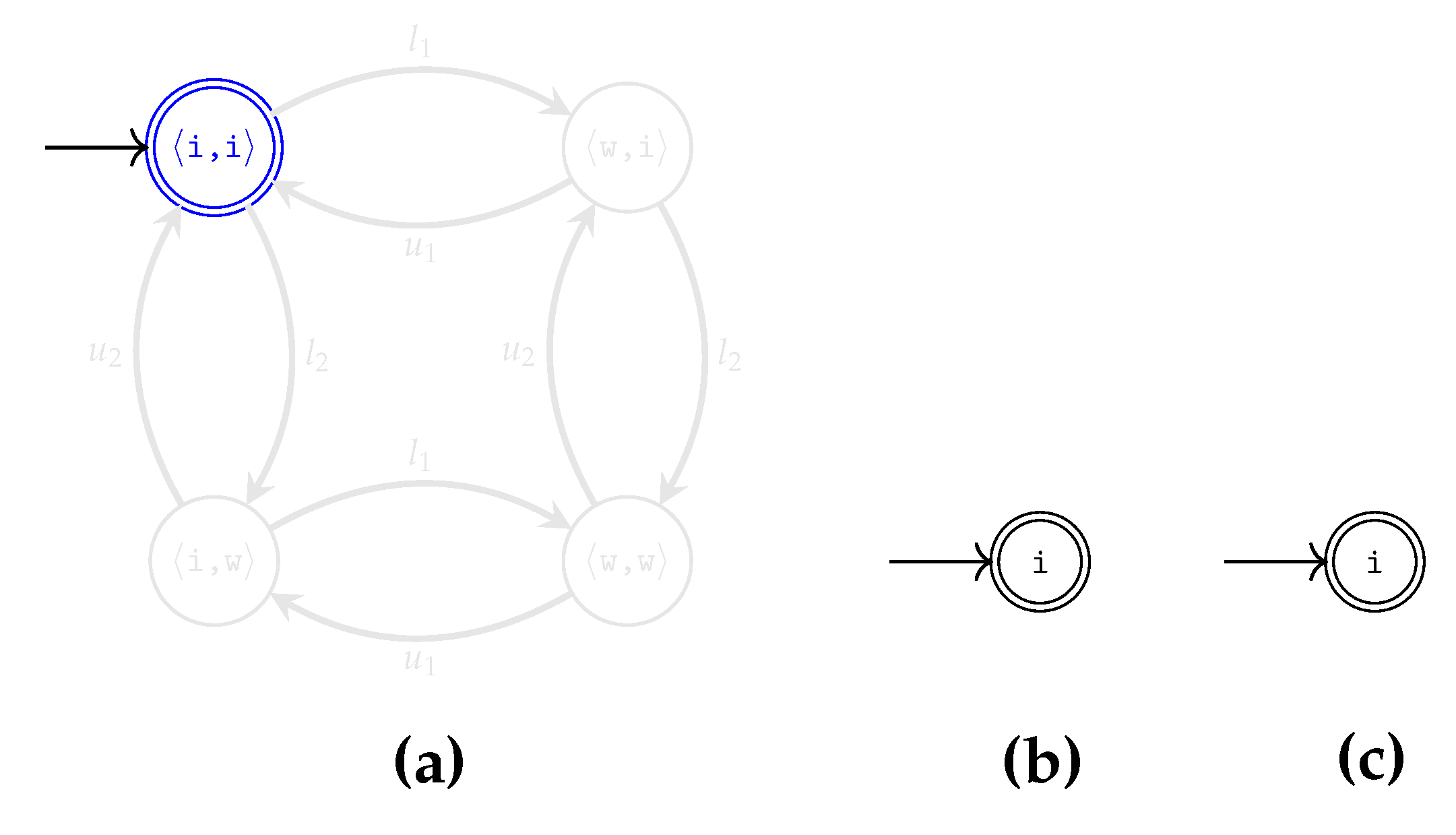
4.2. The Modular Plant Learner
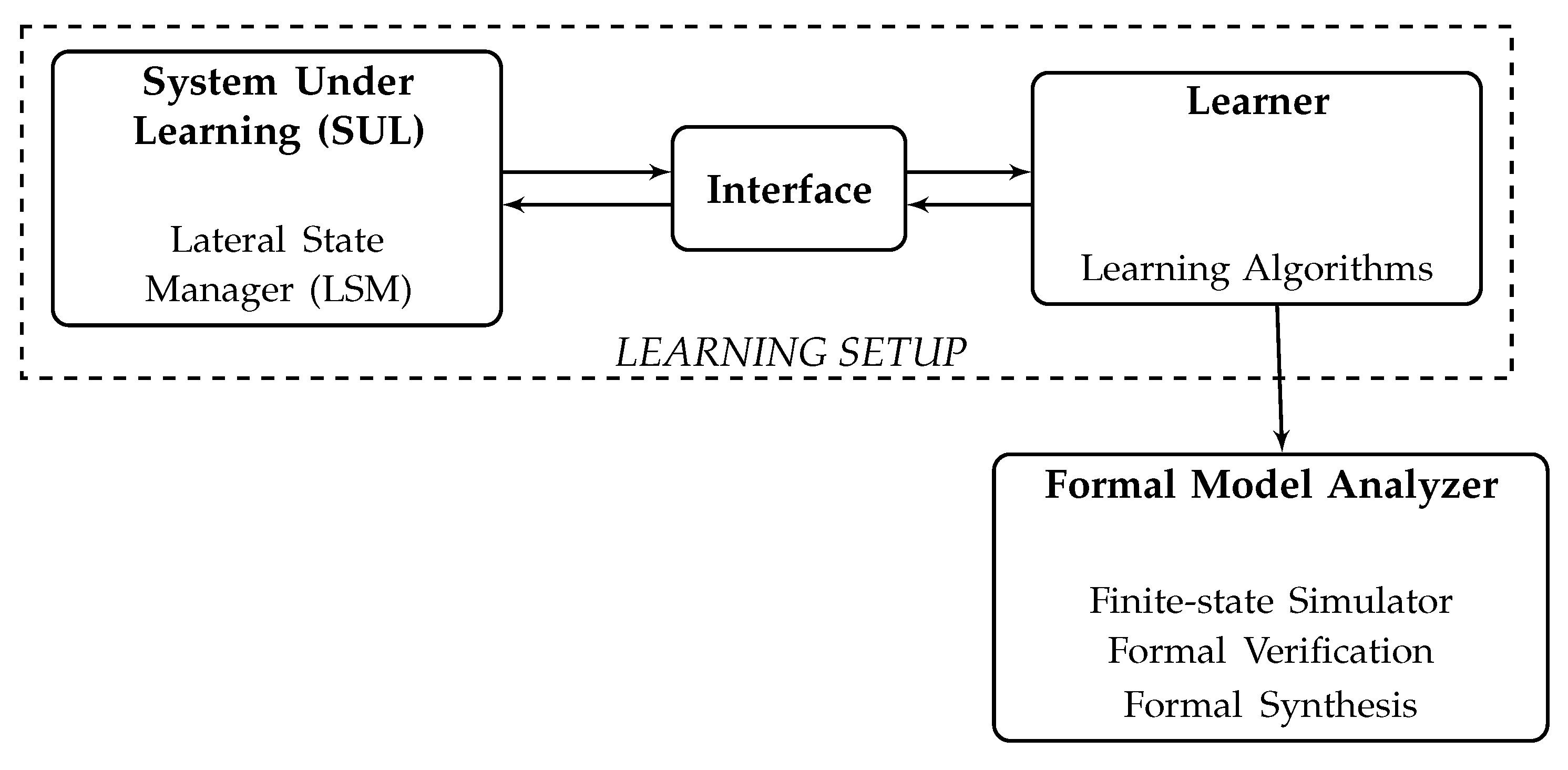
5. Method: The Learning Setup
5.1. Abstracting the Code
- Listing 1. A small illustrative example.
|
- Listing 2. Abstracted version of Listing 1.
|
5.2. Interaction with the SUL
- Enable communication between MIDES and MATLAB,
- Provide information to MIDES on how to execute the LSM and observe the output.
6. Results
6.1. Learning with
6.2. Learning with MPL
7. Evaluation
7.1. Learning Complexity
7.2. Alphabet Reduction
8. Model Validation
Threats to Validity
9. Insights and Discussion
9.1. Towards Formal Software Development
Continuous Formal Development
9.2. Practical Challenges
9.2.1. Interaction with the SUL
9.2.2. Efficiency of the Learning Algorithms
9.2.3. States vs. Events
9.3. Software Reengineering and Reverse Engineering
10. Conclusions
- The language minimization of the model learned by MPL is very similar to the original model of the LSM.
- Manual comparison of the learned models to a manually developed model of the LSM indicated close similarity.
- Simulating the learned automata in Supremica and comparing to the simulation of the actual code in MATLAB/Simulink showed no obvious discrepancies.
- A known bug in the development code was found also in the learned models.
Author Contributions
Funding
Institutional Review Board Statement
Informed Consent Statement
Data Availability Statement
Acknowledgments
Conflicts of Interest
References
- Litman, T. Autonomous Vehicle Implementation Predictions; Victoria Transport Policy Institute: Victoria, BC, Canada, 2020. [Google Scholar]
- Koopman, P.; Wagner, M. Autonomous vehicle safety: An interdisciplinary challenge. IEEE Intell. Transp. Syst. Mag. 2017, 9, 90–96. [Google Scholar] [CrossRef]
- Broy, M.; Kruger, I.H.; Pretschner, A.; Salzmann, C. Engineering automotive software. Proc. IEEE 2007, 95, 356–373. [Google Scholar] [CrossRef]
- Broy, M. Challenges in Automotive Software Engineering. In ICSE ’06: Proceedings of the 28th International Conference on Software engineering, Shanghai, China, 20–28 May 2006; Association for Computing Machinery: New York, NY, USA, 2006; pp. 33–42. [Google Scholar] [CrossRef]
- Liebel, G.; Marko, N.; Tichy, M.; Leitner, A.; Hansson, J. Model-based engineering in the embedded systems domain: An industrial survey on the state-of-practice. Softw. Syst. Model. 2018, 17, 91–113. [Google Scholar] [CrossRef]
- Charfi Smaoui, A.; Liu, F.; Mraidha, C. A Model Based System Engineering Methodology for an Autonomous Driving System Design. In Proceedings of the 25th ITS World Congress, Copenhagen, Denmark, 17–21 September 2018; HAL: Copenhagen, Denmark, 2018. [Google Scholar]
- Struss, P.; Price, C. Model-based systems in the automotive industry. AI Mag. 2003, 24, 17. [Google Scholar]
- Di Sandro, A.; Kokaly, S.; Salay, R.; Chechik, M. Querying Automotive System Models and Safety Artifacts: Tool Support and Case Study. J. Automot. Softw. Eng. 2020, 1, 34–50. [Google Scholar] [CrossRef]
- The MathWorks Inc. MATLAB. Available online: https://se.mathworks.com/products/matlab.html (accessed on 17 February 2020).
- Friedman, J. MATLAB/Simulink for automotive systems design. In Proceedings of the Design Automation & Test in Europe Conference, Munich, Germany, 6–10 March 2006; Volume 1, pp. 1–2. [Google Scholar]
- Utting, M.; Legeard, B. Practical Model-Based Testing; Morgan Kaufmann: San Francisco, CA, USA, 2007. [Google Scholar]
- Altinger, H.; Wotawa, F.; Schurius, M. Testing Methods Used in the Automotive Industry: Results from a Survey. In Proceedings of the 2014 Workshop on Joining AcadeMiA and Industry Contributions to Test Automation and Model-Based Testing, JAMAICA 2014, San Jose, CA, USA, 21 July 2014; Association for Computing Machinery: New York, NY, USA, 2014; pp. 1–6. [Google Scholar] [CrossRef]
- Kalra, N.; Paddock, S.M. Driving to safety: How many miles of driving would it take to demonstrate autonomous vehicle reliability? Transp. Res. Part A Policy Pract. 2016, 94, 182–193. [Google Scholar] [CrossRef]
- Luckcuck, M.; Farrell, M.; Dennis, L.A.; Dixon, C.; Fisher, M. Formal specification and verification of autonomous robotic systems: A survey. ACM Comput. Surv. 2019, 52, 1–41. [Google Scholar] [CrossRef] [Green Version]
- Guiochet, J.; Machin, M.; Waeselynck, H. Safety-critical advanced robots: A survey. Robot. Auton. Syst. 2017, 94, 43–52. [Google Scholar] [CrossRef] [Green Version]
- The MathWorks Inc. Simulink Design Verifier. Available online: https://se.mathworks.com/products/simulink-design-verifier.html (accessed on 17 February 2020).
- The MathWorks Inc. Polyspace Products. Available online: https://se.mathworks.com/products/polyspace.html (accessed on 17 February 2020).
- Leitner-Fischer, F.; Leue, S. Simulink Design Verifier vs. SPIN: A Comparative Case Study. 2008. Available online: http://kops.uni-konstanz.de/handle/123456789/21292 (accessed on 17 February 2020).
- Schürenberg, M. Scalability Analysis of the Simulink Design Verifier on an Avionic System. Bachelor Thesis, Hamburg University of Technology, Hamburg, Germany, 2012. [Google Scholar]
- Selvaraj, Y.; Ahrendt, W.; Fabian, M. Verification of Decision Making Software in an Autonomous Vehicle: An Industrial Case Study. In Formal Methods for Industrial Critical Systems; Springer: Cham, Switzerland, 2019; pp. 143–159. [Google Scholar]
- Mashkoor, A.; Kossak, F.; Egyed, A. Evaluating the suitability of state-based formal methods for industrial deployment. Softw. Pract. Exp. 2018, 48, 2350–2379. [Google Scholar] [CrossRef]
- Baier, C.; Katoen, J.P. Principles of Model Checking; MIT Press: Cambridge, MA, USA, 2008. [Google Scholar]
- Ramadge, P.J.; Wonham, W.M. The control of discrete event systems. Proc. IEEE 1989, 77, 81–98. [Google Scholar] [CrossRef]
- Liu, X.; Yang, H.; Zedan, H. Formal methods for the re-engineering of computing systems: A comparison. In Proceedings of the Twenty-First Annual International Computer Software and Applications Conference (COMPSAC’97), Washington, DC, USA, 13–15 August 1997; pp. 409–414. [Google Scholar]
- Angluin, D. Learning regular sets from queries and counterexamples. Inf. Comput. 1987, 75, 87–106. [Google Scholar] [CrossRef] [Green Version]
- Steffen, B.; Howar, F.; Merten, M. Introduction to active automata learning from a practical perspective. In International School on Formal Methods for the Design of Computer, Communication and Software Systems; Springer: Berlin/Heidelberg, Germany, 2011; pp. 256–296. [Google Scholar]
- Aarts, F. Tomte: Bridging the Gap between Active Learning and Real-World Systems Title of the Work. Ph.D. Thesis, Radboud University, Nijmegen, The Netherlands, 2014. [Google Scholar]
- Cassel, S.; Howar, F.; Jonsson, B.; Steffen, B. Active learning for extended finite state machines. Form. Asp. Comput. 2016, 28, 233–263. [Google Scholar] [CrossRef]
- Howar, F.; Steffen, B. Active automata learning in practice. In Machine Learning for Dynamic Software Analysis: Potentials and Limits; Springer: Cham, Switzerland, 2018; pp. 123–148. [Google Scholar]
- Farooqui, A.; Hagebring, F.; Fabian, M. Active Learning of Modular Plant Models. IFAC-PapersOnLine 2020, 53, 296–302. [Google Scholar] [CrossRef]
- de la Higuera, C. Grammatical Inference: Learning Automata and Grammars; Cambridge University Press: New York, NY, USA, 2010. [Google Scholar]
- Isberner, M.; Howar, F.; Steffen, B. The open-source LearnLib: A Framework for Active Automata Learning. In Proceedings of the International Conference on Computer Aided Verification; Springer: Cham, Switzerland, 2015; pp. 487–495. [Google Scholar]
- Cassandras, C.G.; Lafortune, S. Introduction to Discrete Event Systems; Springer: New York, NY, USA, 2009. [Google Scholar]
- Selvaraj, Y.; Farooqui, A.; Panahandeh, G.; Fabian, M. Automatically Learning Formal Models: An Industrial Case from Autonomous Driving Development. In Proceedings of the 23rd ACM/IEEE International Conference on Model Driven Engineering Languages and Systems: Companion Proceedings, MODELS ’20, Virtual Event Canada, 16–23 October 2020; Association for Computing Machinery: New York, NY, USA, 2020. [Google Scholar] [CrossRef]
- Farooqui, A.; Hagebring, F.; Fabian, M. MIDES: A Tool for Supervisor Synthesis via Active Learning. In Proceedings of the 2021 IEEE 17th International Conference on Automation Science and Engineering (CASE), Lyon, France, 23–27 August 2021; pp. 792–797. [Google Scholar] [CrossRef]
- Farooqui, A.; Fabian, M. Synthesis of Supervisors for Unknown Plant Models Using Active Learning. In Proceedings of the 2019 IEEE 15th International Conference on Automation Science and Engineering (CASE), Vancouver, BC, Canada, 22–26 August 2019; pp. 502–508. [Google Scholar]
- Corbett, J.C.; Dwyer, M.B.; Hatcliff, J.; Laubach, S.; Pasareanu, C.S.; Zheng, H. Bandera: Extracting finite-state models from Java source code. In Proceedings of the 2000 International Conference on Software Engineering, ICSE 2000 the New Millennium, Limerick, Ireland, 4–11 June 2000; pp. 439–448. [Google Scholar]
- Holzmann, G.J. From code to models. In Proceedings of the Second International Conference on Application of Concurrency to System Design, Newcastle upon Tyne, UK, 25–29 June 2001; pp. 3–10. [Google Scholar]
- Holzmann, G.J.; Smith, M.H. A practical method for verifying event-driven software. In Proceedings of the 1999 International Conference on Software Engineering (IEEE Cat. No. 99CB37002), Los Angeles, CA, USA, 16–22 May 1999; pp. 597–607. [Google Scholar]
- Reicherdt, R.; Glesner, S. Formal verification of discrete-time MATLAB/Simulink models using Boogie. In Proceedings of the International Conference on Software Engineering and Formal Methods, Grenoble, France, 1–5 September 2014; Springer: Cham, Switzerland, 2014; pp. 190–204. [Google Scholar]
- de Moura, L.; Bjørner, N. Z3: An Efficient SMT Solver. In Tools and Algorithms for the Construction and Analysis of Systems; Ramakrishnan, C.R., Rehof, J., Eds.; Springer: Berlin/Heidelberg, Germany, 2008; pp. 337–340. [Google Scholar]
- Araiza-Illan, D.; Eder, K.; Richards, A. Formal verification of control systems’ properties with theorem proving. In Proceedings of the 2014 UKACC International Conference on Control (CONTROL), Loughborough, UK, 9–11 July 2014; pp. 244–249. [Google Scholar]
- Fang, H.; Guo, J.; Zhu, H.; Shi, J. Formal verification and simulation: Co-verification for subway control systems. In Proceedings of the 2012 Sixth International Symposium on Theoretical Aspects of Software Engineering, Beijing, China, 4–6 July 2012; pp. 145–152. [Google Scholar]
- Jonsson, B. Learning of Automata Models Extended with Data. In Formal Methods for Eternal Networked Software Systems, Proceedings of the 11th International School on Formal Methods for the Design of Computer, Communication and Software Systems, SFM 2011, Bertinoro, Italy, 13–18 June 2011. Advanced Lectures; Advanced Lectures; Springer: Berlin/Heidelberg, Germany, 2011; pp. 327–349. [Google Scholar] [CrossRef] [Green Version]
- Aarts, F.; Schmaltz, J.; Vaandrager, F. Inference and Abstraction of the Biometric Passport. In Leveraging Applications of Formal Methods, Verification, and Validation; Margaria, T., Steffen, B., Eds.; Springer: Berlin/Heidelberg, Germany, 2010; pp. 673–686. [Google Scholar]
- Aarts, F.; De Ruiter, J.; Poll, E. Formal models of bank cards for free. In Proceedings of the 2013 IEEE Sixth International Conference on Software Testing, Verification and Validation Workshops, Luxembourg, 18–22 March 2013; pp. 461–468. [Google Scholar]
- Smeenk, W.; Moerman, J.; Vaandrager, F.; Jansen, D.N. Applying Automata Learning to Embedded Control Software. In Formal Methods and Software Engineering; Butler, M., Conchon, S., Zaïdi, F., Eds.; Springer: Cham, Switzerland, 2015; pp. 67–83. [Google Scholar]
- Merten, M.; Isberner, M.; Howar, F.; Steffen, B.; Margaria, T. Automated learning setups in automata learning. In Proceedings of the International Symposium on Leveraging Applications of Formal Methods, Verification and Validation, Heraklion, Greece, 15–18 October 2012; Springer: Berlin/Heidelberg, Germany, 2012; pp. 591–607. [Google Scholar]
- Merten, M. Active Automata Learning for Real Life Applications. Ph.D Thesis, TU Dortmund University, Dortmund, Germany, 2013. [Google Scholar]
- Kunze, S.; Mostowski, W.; Mousavi, M.R.; Varshosaz, M. Generation of failure models through automata learning. In Proceedings of the 2016 Workshop on Automotive Systems/Software Architectures (WASA), Venice, Italy, 5–8 April 2016; pp. 22–25. [Google Scholar]
- Meinke, K.; Sindhu, M.A. LBTest: A learning-based testing tool for reactive systems. In Proceedings of the 2013 IEEE Sixth International Conference on Software Testing, Verification and Validation, Luxembourg, 18–20 March 2013; pp. 447–454. [Google Scholar]
- Zhang, H.; Feng, L.; Li, Z. A Learning-Based Synthesis Approach to the Supremal Nonblocking Supervisor of Discrete-Event Systems. IEEE Trans. Autom. Control 2018, 63, 3345–3360. [Google Scholar] [CrossRef]
- Chow, T. Testing Software Design Modeled by Finite-State Machines. IEEE Trans. Softw. Eng. 1978, 4, 178–187. [Google Scholar] [CrossRef]
- The MathWorks Inc.Java Engine API Summary. Available online: https://se.mathworks.com/help/matlab/matlab_external/get-started-with-matlab-engine-api-for-java.html (accessed on 17 February 2020).
- Berg, T. Regular Inference for Reactive Systems. Ph.D. Thesis, Uppsala University, Uppsala, Sweden, 2006. [Google Scholar]
- Czerny, M.X. Learning-Based Software Testing: Evaluation of Angluin’s L* Algorithm and Adaptations in Practice. Bachelor Thesis, Karlsruhe Institute of Technology, Department of Informatics Institute for Theoretical Computer Science, Karlsruhe, Germany, 2014. [Google Scholar]
- Zita, A.; Mohajerani, S.; Fabian, M. Application of formal verification to the lane change module of an autonomous vehicle. In Proceedings of the 2017 13th IEEE Conference on Automation Science and Engineering (CASE), Xi’an, China, 20–23 August 2017; pp. 932–937. [Google Scholar]
- Malik, R.; Akesson, K.; Flordal, H.; Fabian, M. Supremica–An Efficient Tool for Large-Scale Discrete Event Systems. IFAC-PapersOnLine 2017, 50, 5794–5799. [Google Scholar] [CrossRef]
- Rausch, A.; Brox, O.; Grewe, A.; Ibe, M.; Jauns-Seyfried, S.; Knieke, C.; Körner, M.; Küpper, S.; Mauritz, M.; Peters, H.; et al. Managed and Continuous Evolution of Dependable Automotive Software Systems. In Proceedings of the 10th Symposium on Automotive Powertrain Control Systems, 7 December 2014; Cramer: Braunschweig, Germany, 2014; pp. 15–51. [Google Scholar]
- Patil, M.; Annamaneni, S.; Model Based System Engineering (MBSE) for Accelerating Software Development Cycle. Technical Report, L&T Technology Services White Paper. 2015. Available online: https://www.ltts.com/sites/default/files/whitepapers/2017-07/wp-model-based-sys-engg.pdf (accessed on 27 December 2021).
- Kubíček, K.; Čech, M.; Škach, J. Continuous enhancement in model-based software development and recent trends. In Proceedings of the 2019 24th IEEE International Conference on Emerging Technologies and Factory Automation (ETFA), Zaragoza, Spain, 10–13 September 2019; pp. 71–78. [Google Scholar]
- Cie, K.M. Agile in Automotive—State of Practice 2015; Study; Kugler Maag Cie: Kornwestheim, Germany, 2015; p. 58. [Google Scholar]
- Monteiro, F.R.; Gadelha, M.Y.R.; Cordeiro, L.C. Boost the Impact of Continuous Formal Verification in Industry. arXiv 2019, arXiv:1904.06152. [Google Scholar]
- Thums, A.; Quante, J. Reengineering embedded automotive software. In Proceedings of the 2012 28th IEEE International Conference on Software Maintenance (ICSM), Trento, Italy, 23–28 September 2012; pp. 493–502. [Google Scholar]
- Schulte-Coerne, V.; Thums, A.; Quante, J. Challenges in reengineering automotive software. In Proceedings of the 2009 13th European Conference on Software Maintenance and Reengineering, Kaiserslautern, Germany, 24–27 March 2009; pp. 315–316. [Google Scholar]
- Malik, R.; Fabian, M.; Åkesson, K. Modelling Large-Scale Discrete-Event Systems Using Modules, Aliases, and Extended Finite-State Automata. IFAC Proc. Vol. 2011, 44, 7000–7005. [Google Scholar] [CrossRef] [Green Version]


Publisher’s Note: MDPI stays neutral with regard to jurisdictional claims in published maps and institutional affiliations. |
© 2022 by the authors. Licensee MDPI, Basel, Switzerland. This article is an open access article distributed under the terms and conditions of the Creative Commons Attribution (CC BY) license (https://creativecommons.org/licenses/by/4.0/).
Share and Cite
Selvaraj, Y.; Farooqui, A.; Panahandeh, G.; Ahrendt, W.; Fabian, M. Automatically Learning Formal Models from Autonomous Driving Software. Electronics 2022, 11, 643. https://doi.org/10.3390/electronics11040643
Selvaraj Y, Farooqui A, Panahandeh G, Ahrendt W, Fabian M. Automatically Learning Formal Models from Autonomous Driving Software. Electronics. 2022; 11(4):643. https://doi.org/10.3390/electronics11040643
Chicago/Turabian StyleSelvaraj, Yuvaraj, Ashfaq Farooqui, Ghazaleh Panahandeh, Wolfgang Ahrendt, and Martin Fabian. 2022. "Automatically Learning Formal Models from Autonomous Driving Software" Electronics 11, no. 4: 643. https://doi.org/10.3390/electronics11040643
APA StyleSelvaraj, Y., Farooqui, A., Panahandeh, G., Ahrendt, W., & Fabian, M. (2022). Automatically Learning Formal Models from Autonomous Driving Software. Electronics, 11(4), 643. https://doi.org/10.3390/electronics11040643