Author Contributions
Conceptualization, D.S., P.S. and S.O.; Data curation, D.S.; Formal analysis, D.S.; Funding acquisition, P.S.; Investigation, D.S.; Methodology, D.S.; Project administration, P.S.; Resources, P.S.; Software, D.S.; Supervision, P.S. and S.O.; Validation, D.S.; Visualization, D.S., P.S. and S.O.; Writing—original draft, D.S.; Writing—review & editing, P.S. and S.O. All authors have read and agreed to the published version of the manuscript.
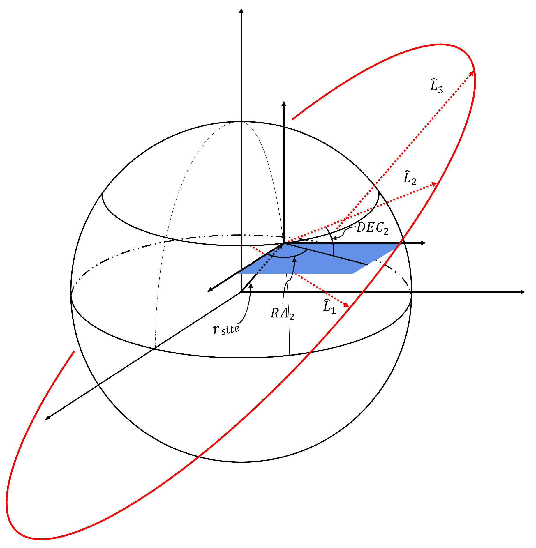
Figure 1.
Geometry of angles-only Initial Orbit Determination.
Figure 1.
Geometry of angles-only Initial Orbit Determination.
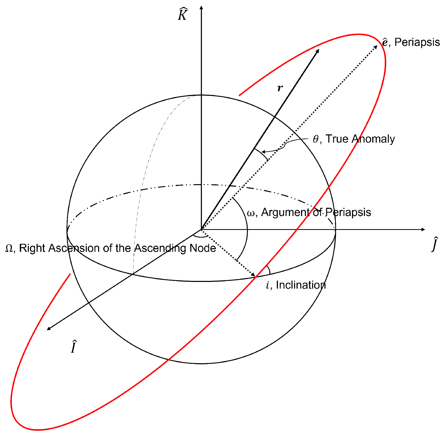
Figure 2.
Geometry classical orbital elements.
Figure 2.
Geometry classical orbital elements.
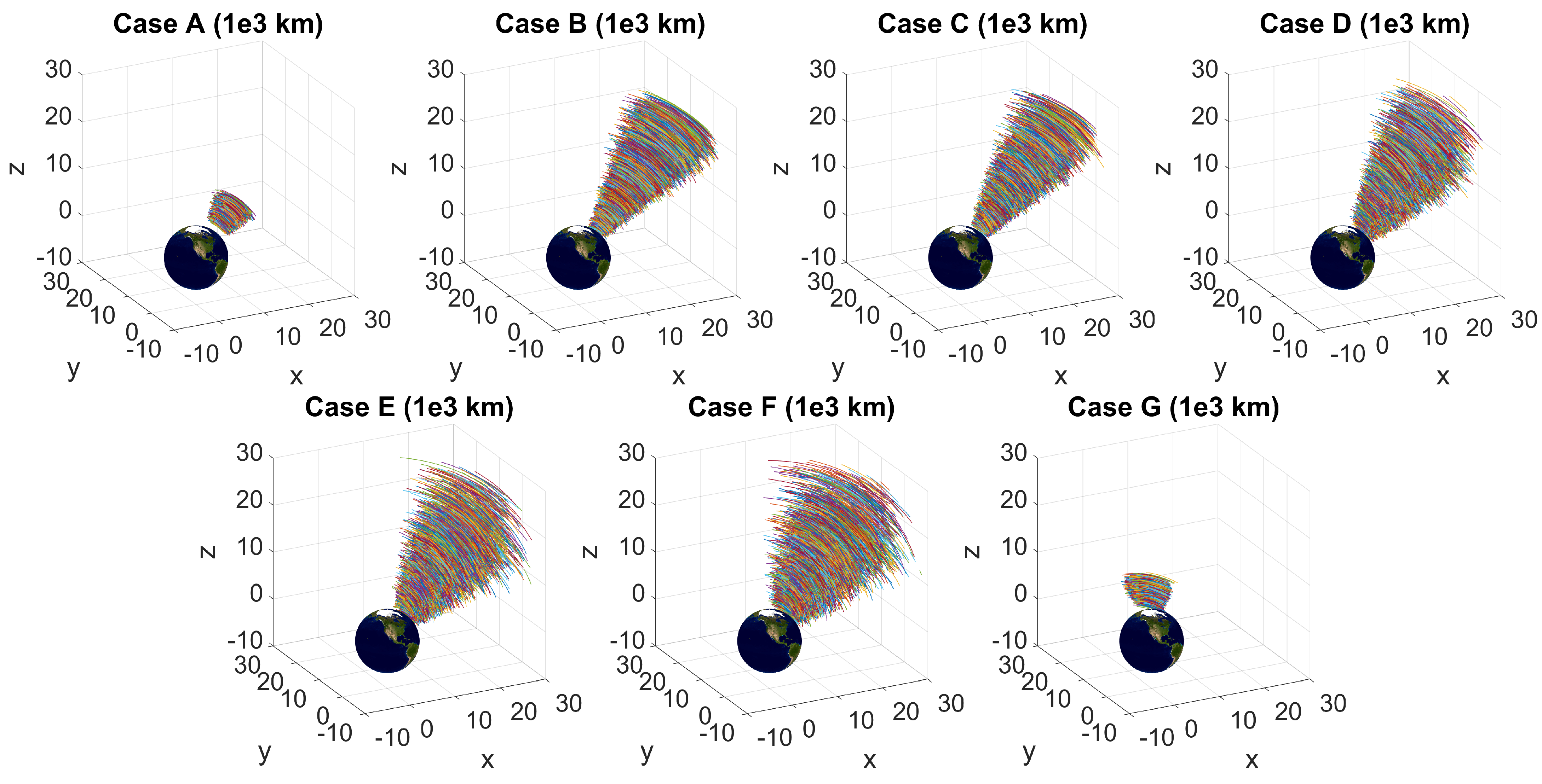
Figure 3.
Orbital arcs for 5000 test orbits of the different orbital case regions.
Figure 3.
Orbital arcs for 5000 test orbits of the different orbital case regions.
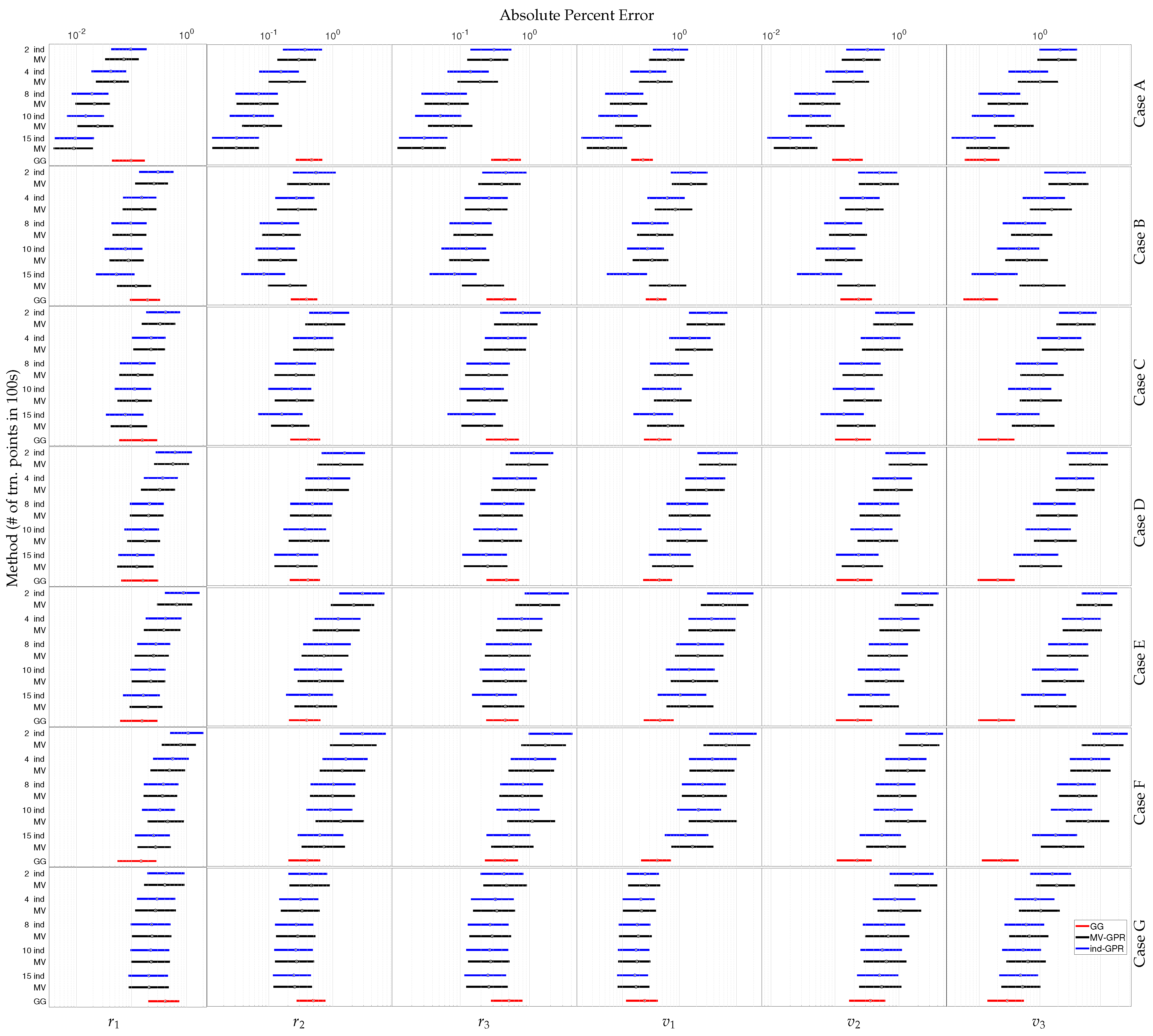
Figure 4.
Given the 5000 testing orbits, the point represents the median APE while the boxes enclose the range of points between the 25th and the 75th quantiles of APE for each Cartesian state given perfect RA and DEC measurements. The GPR methods are listed ind-GPR (blue) then MV-GPR (black) and are ordered by number of training points—200, 400, 800, 1000, and 1500—listed in 100 s. The Gauss–Gibbs results are labeled GG and shown in (red).
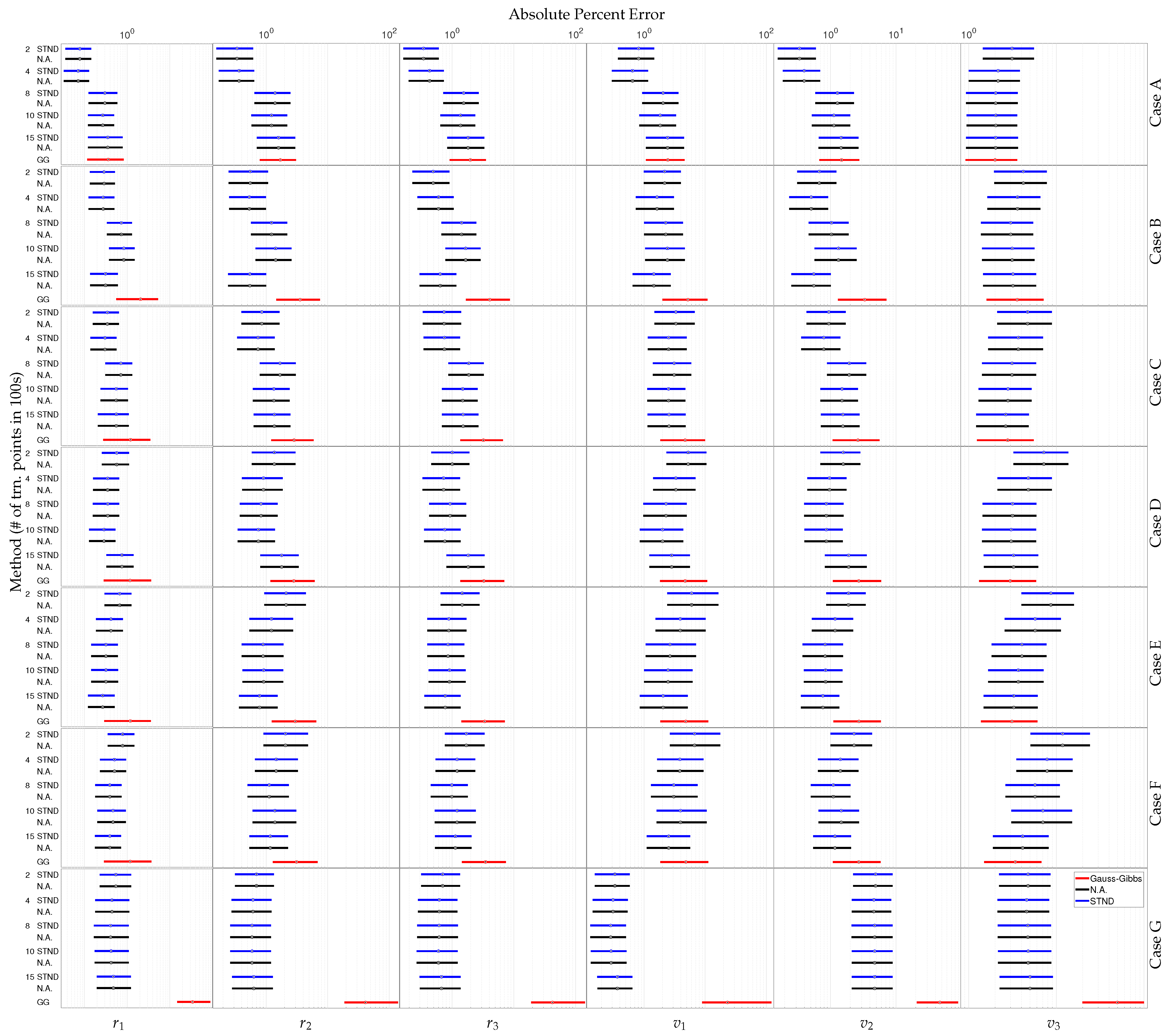
Figure 5.
The point represents the median APE while the boxes enclose the range of points between the 25th and the 75th quantiles of APE for each Cartesian state given uncertain RA and DEC measurements. The GPR methods are listed STND. (blue) Then, N.A. (black) and are ordered by number of training points—200, 400, 800, 1000, and 1500—listed in 100s. The Gauss–Gibbs results are labeled GG and shown in (red).
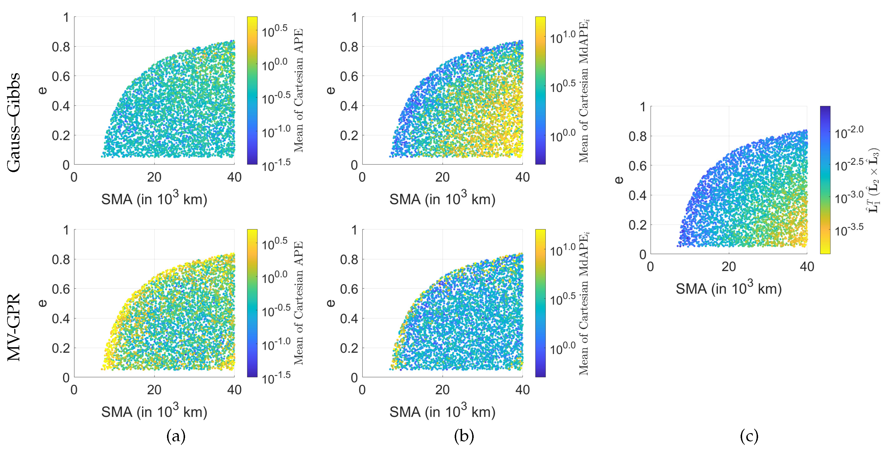
Figure 6.
Effects of orbit shape on GPR predictions for Case C: (a) average of the Cartesian APE of the GPR solution given perfect measurements, (b) the average MdAPE given noisy measurements, (c) the coplanarity of the lines-of-sight. Colorbars represent range for the 99% of points to increase readability in the presence of outliers.
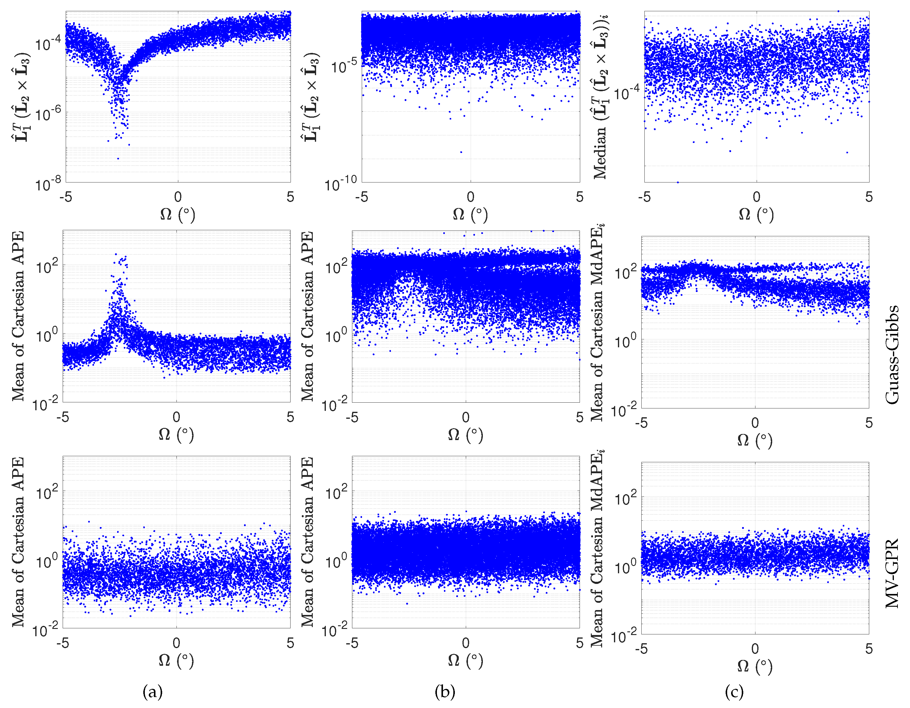
Figure 7.
Effects of coplanarity on Gauss–Gibbs and MV-GPR IOD solutions. (a) scalar triple product of the lines-of-sight and average of the Cartesian APE versus true given perfect measurements. (b) scalar triple product and average of the Cartesian APE versus true given noisy measurements. (c) median scalar triple product and average of the MdAPE versus true for each set of five random samples of the 5000 test orbits.
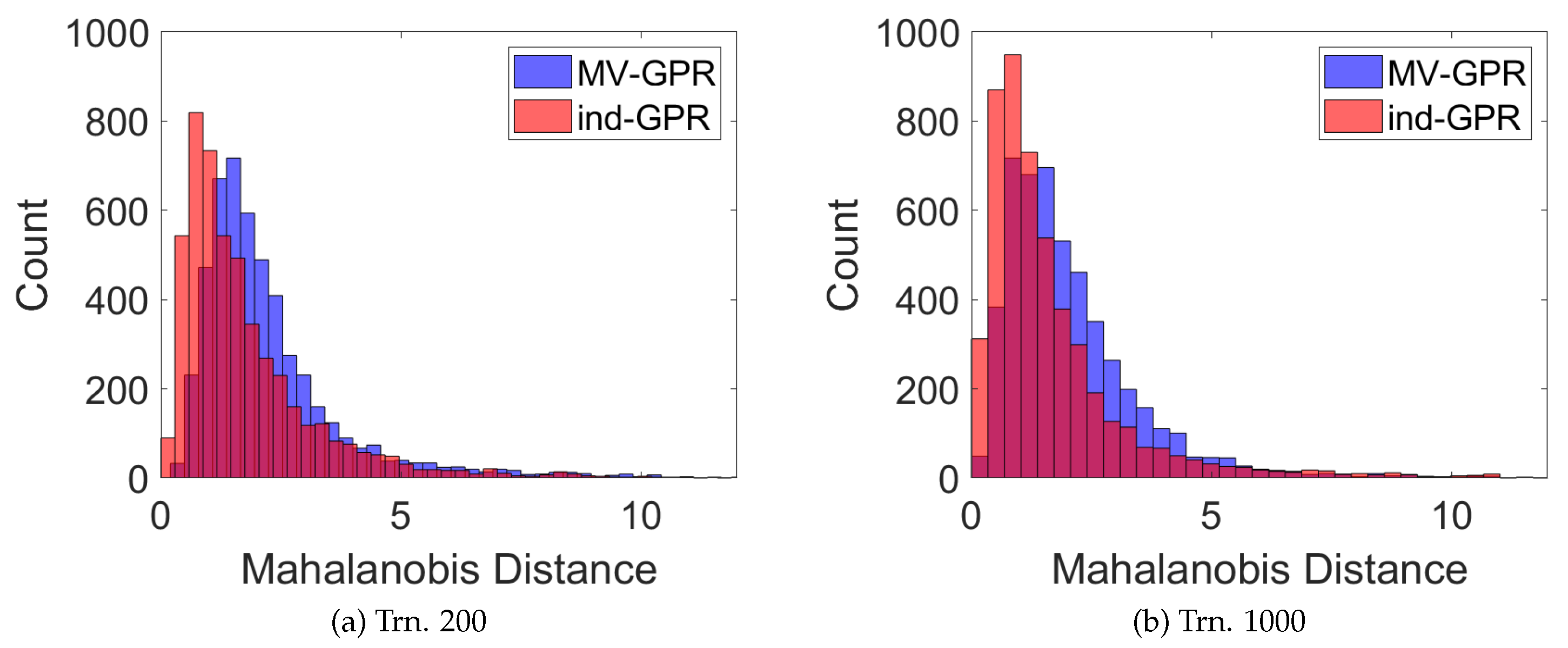
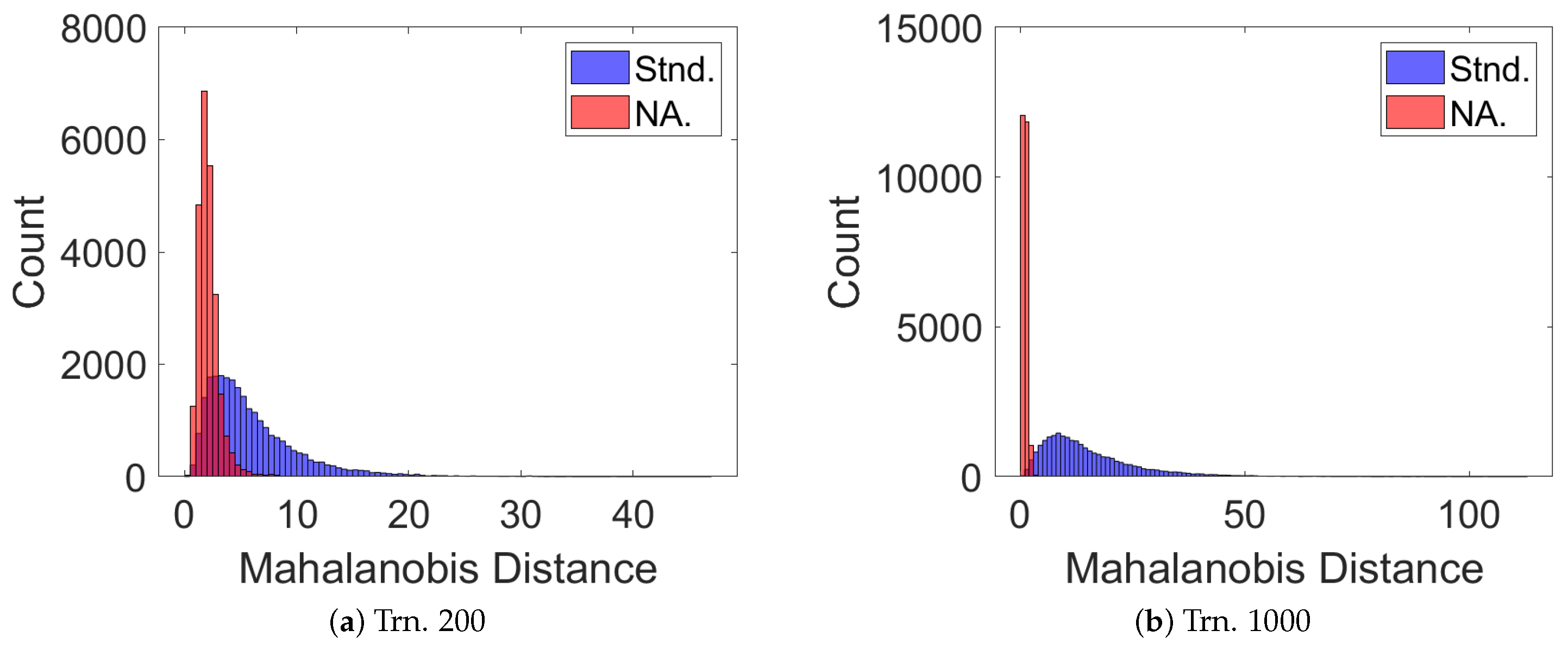
Figure 8.
The Mahalanobis distance from the true state to the GPR-predicted mean given the GPR-predicted covariance (a) 200 and (b) 1000 given perfect RA and DEC measurements.
Figure 8.
The Mahalanobis distance from the true state to the GPR-predicted mean given the GPR-predicted covariance (a) 200 and (b) 1000 given perfect RA and DEC measurements.
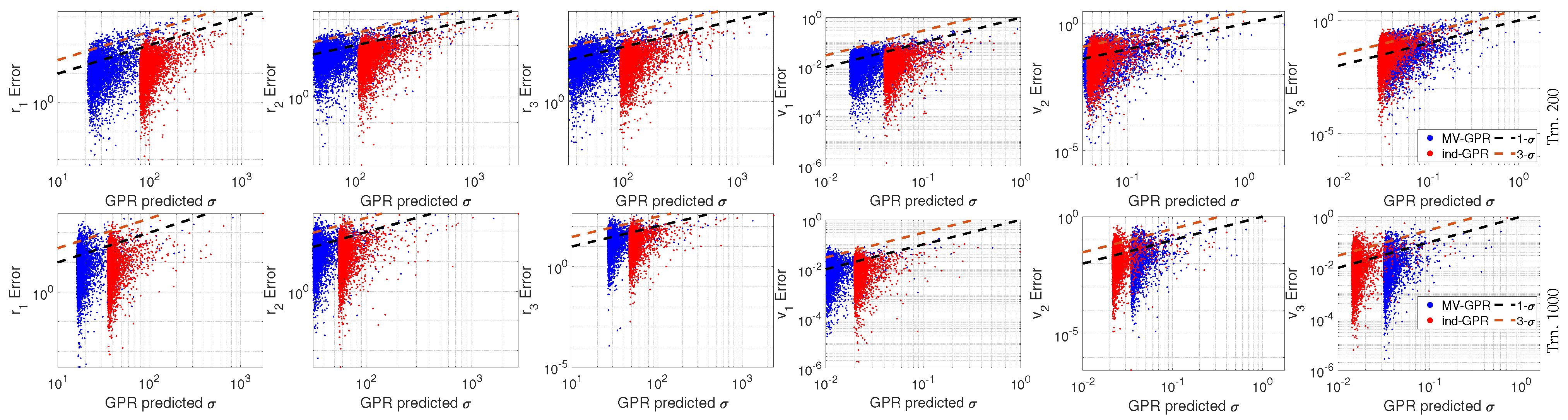
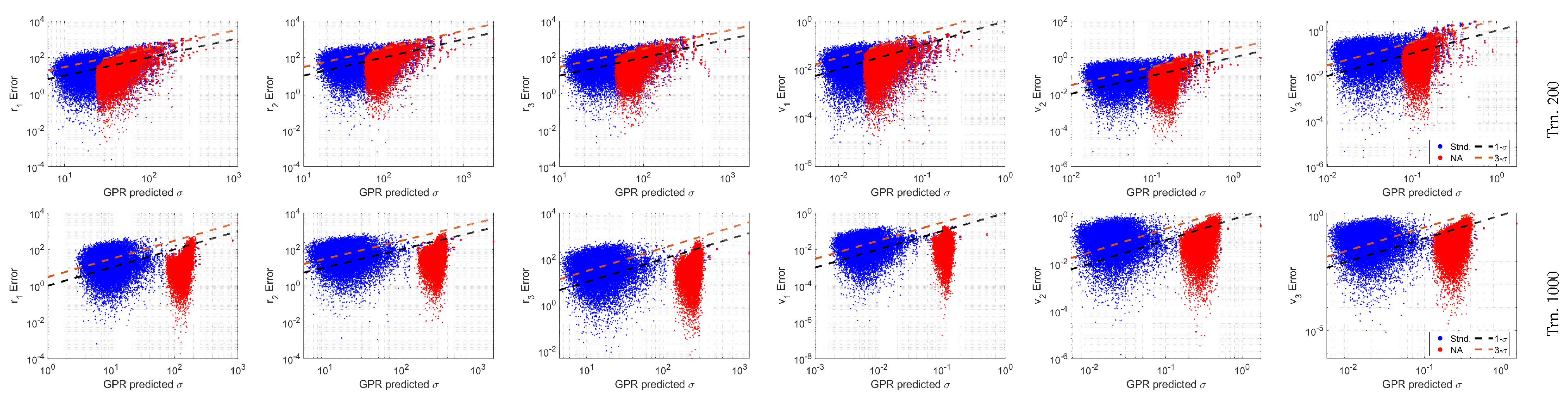
Figure 9.
Predicted standard deviation versus the error between the predicted mean and the true Cartesian state given perfect RA and DEC measurements.
Figure 9.
Predicted standard deviation versus the error between the predicted mean and the true Cartesian state given perfect RA and DEC measurements.
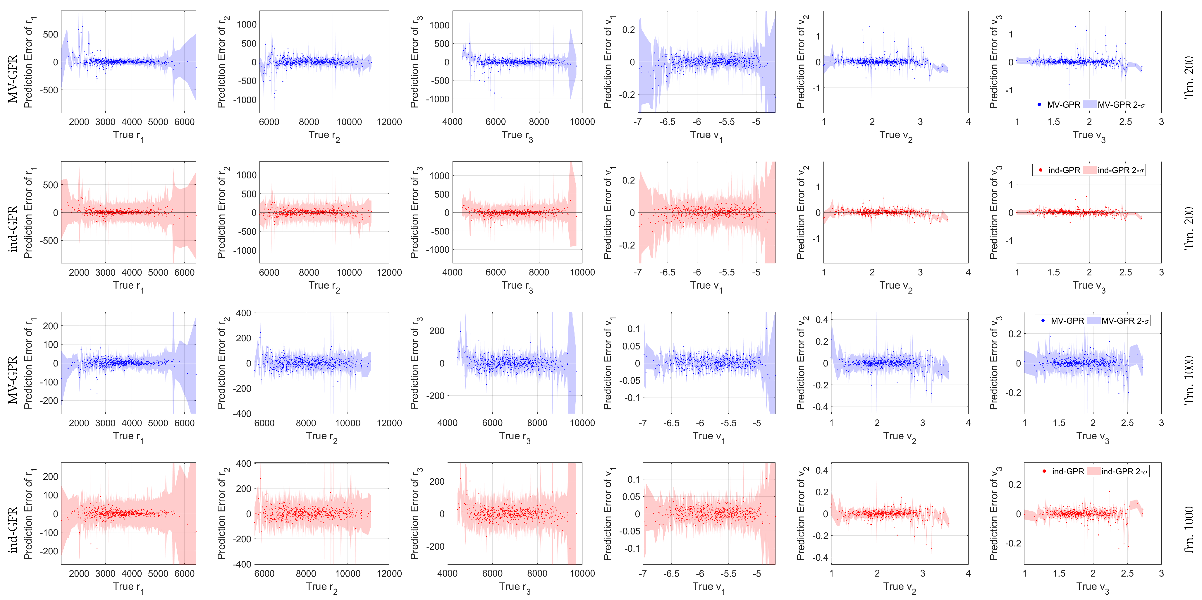
Figure 10.
Cartesian state versus the GPR output error with accompanying 3- bounds for a 500 point random sub-sample of the 5000 test orbits. Note the differing y-scale between the training levels.
Figure 10.
Cartesian state versus the GPR output error with accompanying 3- bounds for a 500 point random sub-sample of the 5000 test orbits. Note the differing y-scale between the training levels.
Figure 11.
The Mahalanobis distance from the true state to the GPR-predicted mean given the GPR-predicted covariance for Case G at training samples of (a) 200 and (b) 1000 given uncertain RA and DEC measurements for the standard MV-GPR (blue) and the noise-aware MV-GPR (red).
Figure 11.
The Mahalanobis distance from the true state to the GPR-predicted mean given the GPR-predicted covariance for Case G at training samples of (a) 200 and (b) 1000 given uncertain RA and DEC measurements for the standard MV-GPR (blue) and the noise-aware MV-GPR (red).
Figure 12.
Predicted standard deviation versus the error between the predicted mean and the true Cartesian state given uncertain angular measurements.
Figure 12.
Predicted standard deviation versus the error between the predicted mean and the true Cartesian state given uncertain angular measurements.
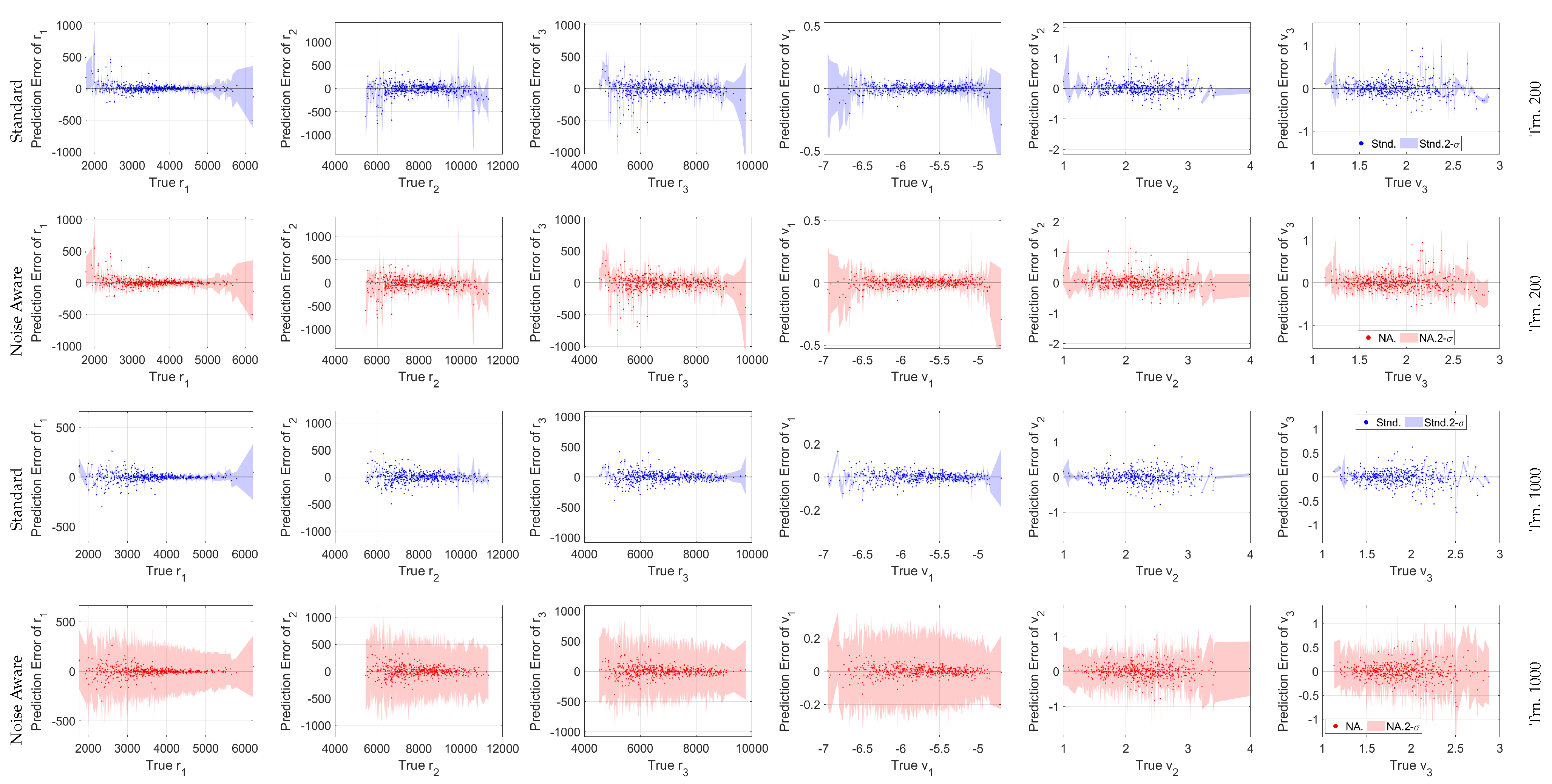
Figure 13.
Cartesian state versus the GPR output error with accompanying 3- bounds for a 500 point random sub-sample of the 25,000 total samples. Note the different y-axis scales between the training levels.
Figure 13.
Cartesian state versus the GPR output error with accompanying 3- bounds for a 500 point random sub-sample of the 25,000 total samples. Note the different y-axis scales between the training levels.
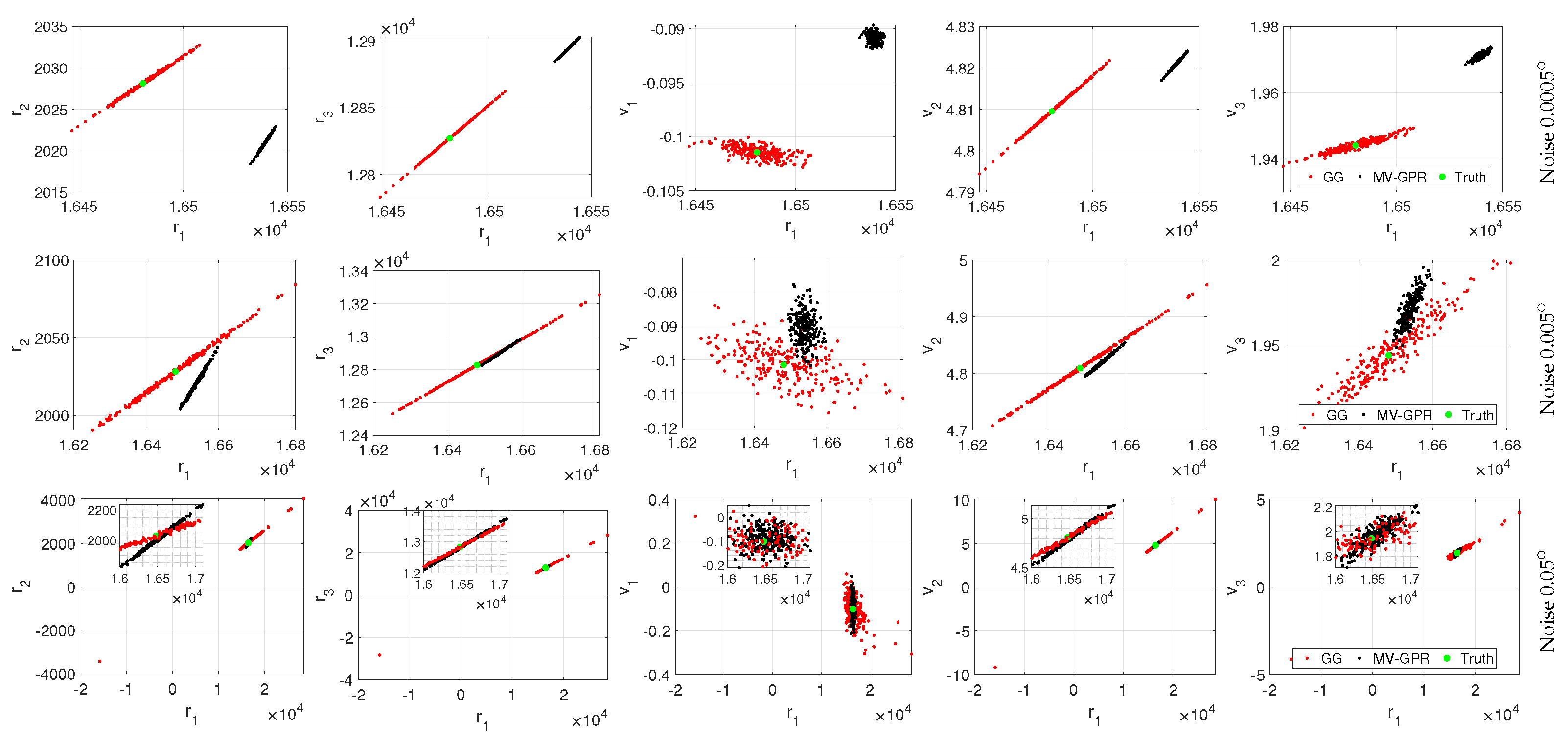
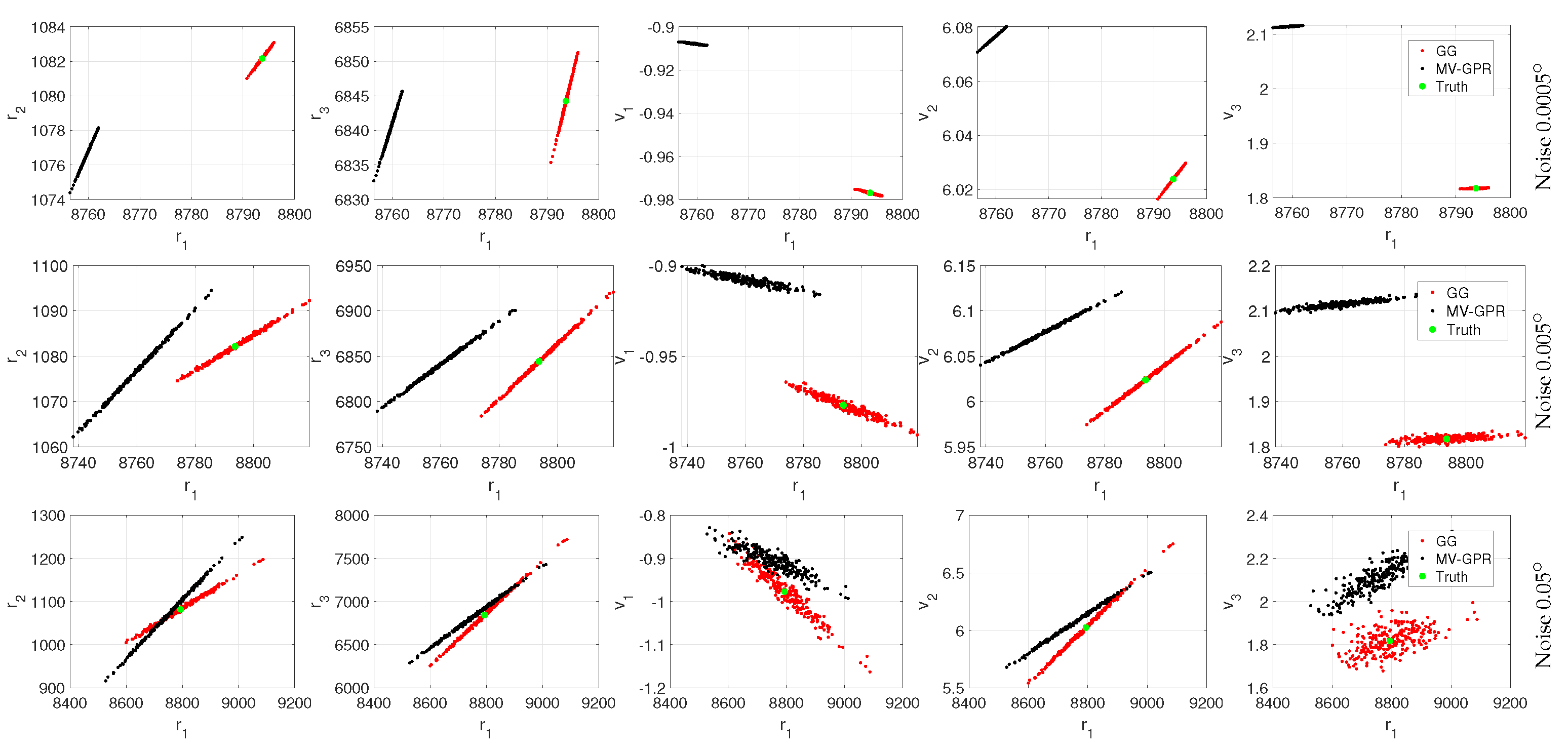
Figure 14.
Qualitative study of Orbit A at various noise levels. The black points are MV-GPR and the red are Gauss–Gibbs predictions, while the green point represents the truth.
Figure 14.
Qualitative study of Orbit A at various noise levels. The black points are MV-GPR and the red are Gauss–Gibbs predictions, while the green point represents the truth.
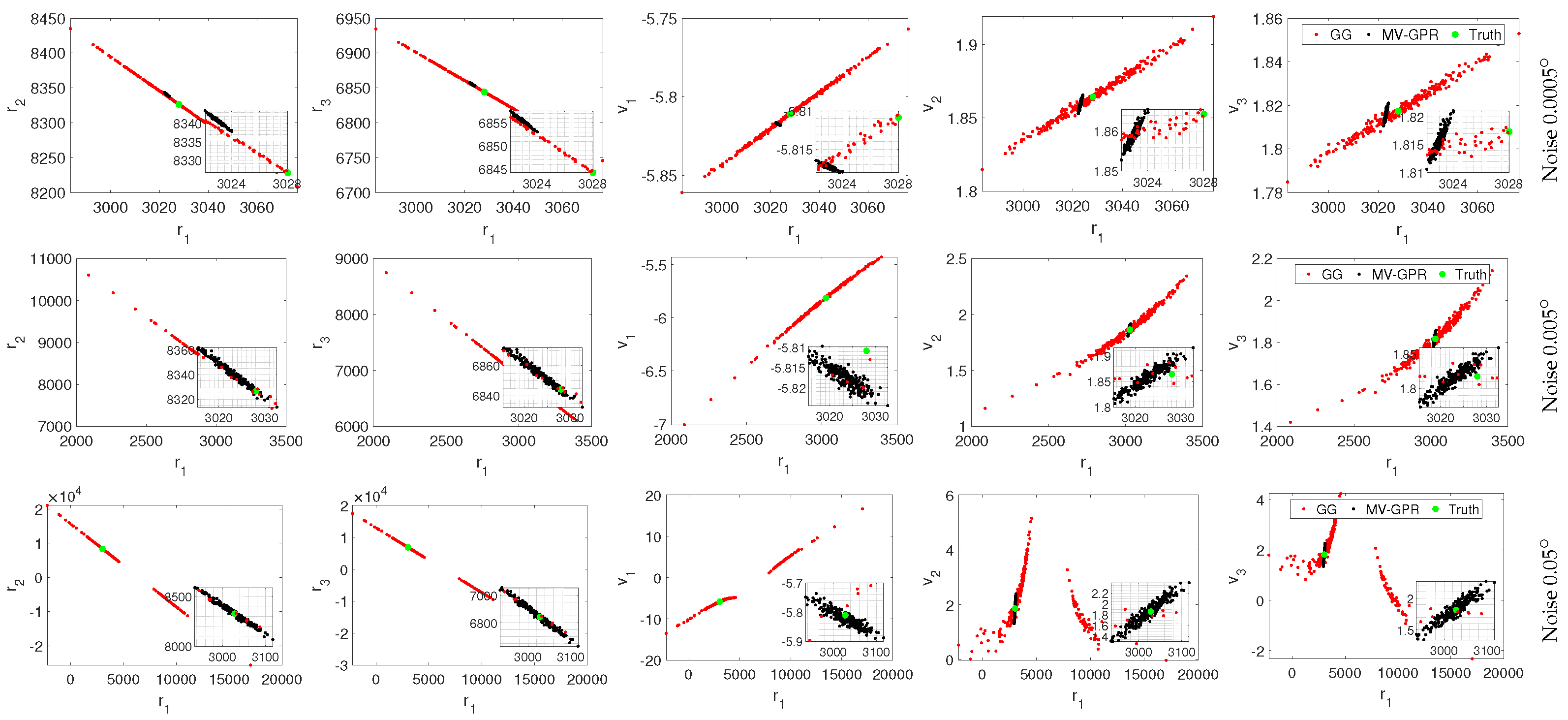
Figure 15.
Qualitative study of Orbit B at various noise levels. The black points are MV-GPR and the red are Gauss–Gibbs predictions, while the green point represents the truth.
Figure 15.
Qualitative study of Orbit B at various noise levels. The black points are MV-GPR and the red are Gauss–Gibbs predictions, while the green point represents the truth.
Figure 16.
Qualitative study of Orbit C at various noise levels. The black points are MV-GPR and the red are Gauss–Gibbs predictions, while the green point represents the truth.
Figure 16.
Qualitative study of Orbit C at various noise levels. The black points are MV-GPR and the red are Gauss–Gibbs predictions, while the green point represents the truth.
Table 1.
Orbital regimes for each case used in GPR study.
Table 1.
Orbital regimes for each case used in GPR study.
| Orbit Case | | e | | | | |
|---|
| Case A | [10,000,16,000] | [0.1, 0.3] | [35, 45] | [305, 315] | [15, 20] | [50, 58] |
| Case B | [6800,40,000] | [0.1, 0.3] | [35, 45] | [305, 315] | [15, 20] | [50, 58] |
| Case C | [6800,40,000] | [0.05, 0.85] | [35, 45] | [305, 315] | [15, 20] | [50, 58] |
| Case D | [6800,40,000] | [0.05, 0.85] | [20, 60] | [305, 315] | [15, 20] | [50, 58] |
| Case E | [6800,40,000] | [0.05, 0.85] | [20, 60] | [295, 325] | [15, 20] | [50, 58] |
| Case F | [6800,40,000] | [0.05, 0.85] | [20, 60] | [295, 325] | [10, 30] | [50, 58] |
| Case G | [10,000,16,000] | [0.1, 0.3] | [35, 45] | [−5, 5] | [15, 20] | [50, 58] |
Table 2.
GPR parameters and their dimesnions in the IOD problem.
Table 2.
GPR parameters and their dimesnions in the IOD problem.
| Input | Output | Hyperparamters |
|---|
| Shared | MV-GPR Specific |
| | | | | |
Table 3.
Median APE for for most accurate model in each orbit case given perfect RA and DEC measurements.
Table 3.
Median APE for for most accurate model in each orbit case given perfect RA and DEC measurements.
| Case | Model | Training Level | Median APE |
|---|
| Case A | ind-GPR | 1500 | 0.0095 | 0.0317 | 0.0303 | 0.0463 | 0.0200 | 0.0850 |
| MV-GPR | 1500 | 0.0089 | 0.0314 | 0.0287 | 0.0563 | 0.0250 | 0.1453 |
| GG | - | 0.0983 | 0.4646 | 0.5004 | 0.2307 | 0.1718 | 0.1243 |
| Case B | ind-GPR | 1500 | 0.0534 | 0.0841 | 0.0830 | 0.1255 | 0.0604 | 0.1844 |
| MV-GPR | 1000 | 0.0881 | 0.1529 | 0.1472 | 0.3337 | 0.1485 | 0.6143 |
| GG | - | 0.1957 | 0.3900 | 0.4321 | 0.4139 | 0.2337 | 0.1174 |
| Case C | ind-GPR | 1500 | 0.0772 | 0.1603 | 0.1549 | 0.3618 | 0.1371 | 0.4269 |
| MV-GPR | 1500 | 0.0972 | 0.2343 | 0.2234 | 0.6334 | 0.2284 | 0.8049 |
| GG | - | 0.1576 | 0.4149 | 0.4546 | 0.4413 | 0.2182 | 0.2059 |
| Case D | ind-GPR | 1500 | 0.1276 | 0.2829 | 0.2371 | 0.6868 | 0.2332 | 0.8654 |
| MV-GPR | 1500 | 0.1257 | 0.2814 | 0.2486 | 0.7773 | 0.2758 | 1.0611 |
| GG | - | 0.1615 | 0.4083 | 0.4645 | 0.4448 | 0.2267 | 0.2026 |
| Case E | ind-GPR | 1500 | 0.1637 | 0.4312 | 0.3371 | 1.0399 | 0.3625 | 1.1506 |
| MV-GPR | 1500 | 0.2004 | 0.5669 | 0.4477 | 1.4703 | 0.5296 | 1.9463 |
| GG | - | 0.1557 | 0.3912 | 0.4458 | 0.4582 | 0.2251 | 0.2112 |
| Case F | ind-GPR | 1500 | 0.2519 | 0.6297 | 0.5063 | 1.2845 | 0.5387 | 1.8216 |
| MV-GPR | 1500 | 0.2734 | 0.7242 | 0.5911 | 1.6985 | 0.6567 | 2.4545 |
| GG | - | 0.1495 | 0.3989 | 0.4391 | 0.4091 | 0.2230 | 0.2350 |
| Case G | ind-GPR | 1500 | 0.2059 | 0.2463 | 0.2513 | 0.1660 | 0.4957 | 0.4790 |
| MV-GPR | 1500 | 0.2089 | 0.2539 | 0.2592 | 0.1734 | 0.5351 | 0.5192 |
| GG | - | 0.4098 | 0.4964 | 0.5066 | 0.2463 | 0.3569 | 0.2897 |
Table 4.
Median APE for for most accurate model in each orbit case given noisy RA and DEC measurements.
Table 4.
Median APE for for most accurate model in each orbit case given noisy RA and DEC measurements.
| Case | Model | Training Level | Median APE |
|---|
| Case A | STND. | 400 | 0.0719 | 0.3647 | 0.4297 | 0.6460 | 0.3972 | 2.1586 |
| N.A. | 400 | 0.0719 | 0.3647 | 0.4299 | 0.6461 | 0.3973 | 2.1576 |
| GG | - | 0.3623 | 1.7049 | 1.9628 | 2.4440 | 1.4774 | 1.9948 |
| Case B | STND. | 1500 | 0.3134 | 0.5451 | 0.6393 | 1.4412 | 0.5567 | 3.1896 |
| N.A. | 1500 | 0.3135 | 0.5452 | 0.6392 | 1.4416 | 0.5571 | 3.1896 |
| GG | - | 2.0710 | 3.5750 | 4.0701 | 5.2170 | 3.3308 | 3.5605 |
| Case C | STND. | 400 | 0.3048 | 0.7412 | 0.7475 | 2.5160 | 0.7924 | 3.6713 |
| N.A. | 400 | 0.3049 | 0.7412 | 0.7476 | 2.5163 | 0.7926 | 3.6715 |
| GG | - | 1.2056 | 2.8494 | 3.2037 | 4.6964 | 2.6248 | 2.7794 |
| Case D | STND. | 1000 | 0.2885 | 0.7497 | 0.7593 | 2.0085 | 0.8639 | 3.0448 |
| N.A. | 1000 | 0.2885 | 0.7498 | 0.7595 | 2.0082 | 0.8639 | 3.0442 |
| GG | - | 1.1726 | 2.8190 | 3.2544 | 4.7066 | 2.7084 | 2.9684 |
| Case E | STND. | 1500 | 0.2687 | 0.7840 | 0.7691 | 2.0489 | 0.7661 | 3.2572 |
| N.A. | 1500 | 0.2687 | 0.7842 | 0.7691 | 2.0486 | 0.7662 | 3.2569 |
| GG | - | 1.1912 | 2.9787 | 3.3680 | 4.8038 | 2.7215 | 3.1105 |
| Case F | STND. | 1500 | 0.3953 | 1.1690 | 1.1260 | 2.5241 | 1.1705 | 4.1178 |
| N.A. | 1500 | 0.3953 | 1.1691 | 1.1256 | 2.5240 | 1.1703 | 4.1165 |
| GG | - | 1.1809 | 3.1280 | 3.4665 | 4.8219 | 2.7099 | 3.3952 |
| Case G | STND. | 400 | 0.4437 | 0.6128 | 0.6185 | 0.3103 | 4.5968 | 4.5697 |
| N.A. | 400 | 0.4438 | 0.6127 | 0.6185 | 0.3102 | 4.5963 | 4.5689 |
| GG | - | 34.0713 | 41.3535 | 42.1487 | 23.1603 | 46.5761 | 49.4980 |
Table 5.
Percentage of errors within –bound for ind- and MV-GPR given perfect input measurements.
Table 5.
Percentage of errors within –bound for ind- and MV-GPR given perfect input measurements.
| Training Level | Model | –Bound | | | | | | |
|---|
| 200 | ind-GPR | | 98.1800 | 96.2200 | 96.9600 | 97.4600 | 66.4000 | 56.1600 |
| 100.0000 | 99.9600 | 99.9800 | 100.0000 | 95.7600 | 91.8400 |
| MV-GPR | | 76.5000 | 73.1200 | 68.3800 | 75.0600 | 64.0600 | 62.1600 |
| 96.1800 | 97.6800 | 96.5600 | 99.7000 | 93.0000 | 92.1800 |
| 1000 | ind-GPR | | 95.0800 | 91.4000 | 91.4400 | 85.7800 | 75.5200 | 68.5600 |
| 99.7400 | 99.7400 | 99.7200 | 99.9000 | 95.6600 | 93.3000 |
| MV-GPR | | 78.9200 | 71.0000 | 69.8800 | 56.3000 | 84.1800 | 86.2000 |
| 97.1200 | 97.8000 | 97.7200 | 96.6000 | 97.5800 | 97.9600 |
Table 6.
Percentage of errors within –bound for standard and noise aware MV-GPR.
Table 6.
Percentage of errors within –bound for standard and noise aware MV-GPR.
| Training Level | Model | –Bound | | | | | | |
|---|
| 200 | STND. | | 53.5880 | 43.6200 | 39.8320 | 50.3240 | 25.0120 | 24.1080 |
| 86.0760 | 82.4120 | 78.9120 | 89.7000 | 57.8480 | 55.9160 |
| N.A. | | 76.7160 | 72.4440 | 69.2400 | 74.6800 | 66.7240 | 66.0720 |
| 98.2960 | 99.2000 | 98.6640 | 99.7680 | 98.7160 | 98.4600 |
| 1000 | STND. | | 36.6560 | 24.4280 | 24.0440 | 22.3760 | 13.6880 | 14.6960 |
| 68.1120 | 55.2760 | 54.4840 | 54.7680 | 35.0440 | 37.1280 |
| N.A. | | 98.3080 | 98.4440 | 98.5120 | 99.4320 | 92.1240 | 92.1600 |
| 100.0000 | 100.0000 | 100.0000 | 100.0000 | 99.9960 | 99.9960 |
Table 7.
Exemplar orbits for qualitative study.
Table 7.
Exemplar orbits for qualitative study.
| Orbit | | e | | | | |
|---|
| Orbit A | 13,000 | 0.2 | 40 | 300 | 17 | 55 |
| Orbit B | 36,000 | 0.5 | 40 | 300 | 17 | 55 |
| Orbit C | 13,000 | 0.2 | 40 | 3 | 17 | 55 |


