Article

Stability Analysis of Chaotic Grey-Wolf Optimized Grid-Tied PV-Hybrid Storage System during Dynamic Conditions

1
Department of Electrical Engineering, NIT Srinagar, Srinagar 190006, India
2
Department of Electrical Engineering, University of Kashmir, Srinagar 190006, India
3
BEARS, University Town, NUS Campus, Singapore 138602, Singapore
4
Department of Electrical Engineering, College of Engineering, King Saud University, Riyadh 11421, Saudi Arabia
*
Authors to whom correspondence should be addressed.
Electronics 2022, 11(4), 567; https://doi.org/10.3390/electronics11040567
Submission received: 30 January 2022 / Revised: 10 February 2022 / Accepted: 11 February 2022 / Published: 13 February 2022
(This article belongs to the Special Issue Environment and Electrical Engineering-Edition 2021)

Abstract

:
This paper presents the stability improvement of the three-phase four-wire (3P-4W) grid-tied PV-hybrid energy storage system (HESS) using chaotic grew wolf optimization (CGWO) for DC bus voltage ( V d c ) and AC bus voltage ( V p c c ) control. The CGWO tuned fractional order proportional–integral (FOPI) controllers reduce the V d c and V p c c variations during diverse, dynamic conditions, i.e., sudden irradiation variations, deep voltage sag/swell, etc. The DC bus is responsible for the current injection/extraction control, maximum PV power extraction, bi-directional power flow, dc second-harmonics component elimination, and active power balance. At the point of common coupling (PCC), the AC bus is accountable for bi-directional power flow and active and reactive power control. The two-level voltage source converter (VSC) is controlled by a novel variable step-size incremental least mean square (VSS-ILMS) in zero voltage regulation (ZVR) mode. Due to its varying step size, VSC control is less prone to noise signals offers better stability, improved convergence rate, dc offset rejection, and tracking speed during dynamics, i.e., large oscillations. A battery and ultracapacitor are coupled to the DC link by buck-boost converters in the HESS. To regulate power transit between the DC bus and the grid, the HESS current control technique is designed to shift frequently from charging to discharging stage and vice versa. The novelty of the PV-HESS system lies in CGWO tuned VSS-ILMS control of VSC, which effectively and efficiently filter out the active fundamental constituents of load current and eliminate dc offset from VSC output. The HESS control maintains the DC bus voltage profile by absorbing and delivering energy (during dynamic conditions) rather than curtailing it. The presented system is simulated in a MATLAB/SIMULINK environment. The simulation results in graphical and numerical forms verify the stable and satisfactory operation of the proposed system as per IEEE519 standard.

1. Introduction

Nowadays, photovoltaic (PV) power generation is widely acclaimed due to its scalable nature and less initial investment than wind energy systems [1]. The grid-tied PV systems offer generation diversification, peak shaving capability, improved reliability, reduced ancillary reserves, improved voltage profile, and reduced transmission losses, etc. Moreover, grid-tied PV systems as distributed generators (DG) lessen the impact of cyber-attack improve power utility security while delivering the critical load [2,3]. In India, the total installed capacity of renewable energy sources (RES) is 103 GW by 2021 (excluding hydropower), in which PV installation is 40%. The total RES installed capacity is expected to grow up to 450 GW by 2030 with a 60% share of PV power (280 GW) [4]. Due to the cost-effectiveness, fewer space constraints, compact size, and ready availability make the grid-tied PV systems suitable for both utility-scale and rooftop plants.
The penetration of RES is increasing day by day in the modern grid to match the energy requirements, which raises many technical issues to be managed before delivering PV power to the grid [5,6]. Considering the cost of PV arrays in PV power generation systems, it is highly desirable to operate them at the highest efficiency. Maximum power point tracking (MPPT) algorithms are utilized for the same. In [7,8] many conventional and artificial intelligence (AI) based MPPT algorithms are given. The transformer-less PV-HESS grid integration is more economical and efficient. However, dual-stage configuration with DC–DC boost converter is best suited for enhanced DC bus stability rather than using single-stage configuration [9,10]. Several technical challenges related to grid integration of PV systems involves designing and control of voltage source converters (VSC), voltage and current harmonics, active and reactive power control, voltage and frequency deviations, stability, power balancing at DC and AC bus, weak grid conditions, PV power fluctuations, bi-directional power flow, lower efficiency, reliability issues, etc. [11,12]. For the satisfactory and healthy operation of grid integration of PV system and to deliver PV power to the grid, technical complications, i.e., stability and power quality issues, must be dealt with.
The stability of the grid-tied PV system significantly relies on DC bus and AC bus stability. The DC bus plays an essential role in managing bi-directional power flow, active power balance, maximum PV power extraction, reducing PV power fluctuations, generating active loss component of current, etc. [13,14]. At the point of common coupling (PCC), the AC bus manages bi-directional active and reactive power flow, islanding detection, low voltage ride through, reactive power compensation, etc. In the case of grid-following converters, the PCC voltage is very much dependent on the grid, which reduces the burden of the AC bus and leaves it with mainly reactive power control [15].
The PI controllers generally control the dc and ac buses due to their simple design procedure, good performance, less computational complexity, and ease of tuning [16,17]. Much artificial intelligence (AI), i.e., fuzzy logic and neural network-based controls, have also been utilized for proportional–integral (PI) controller gain tuning, which increases the system’s complexity [18,19]. Many metaheuristic optimization techniques (MOTs) have been implemented in an offline mode to deliver optimal gains of the PI controller [14,20,21,22,23]. The fractional-order PI controller offers enhanced performance than the PI controller due to its non-integer integral gain. The gains of fractional-order PI (FOPI) can be obtained by using MOTs, i.e., salp swarm optimization (SSO), chaotic grey wolf optimization (CGWO), and many more [20,23]. The increased tuning parameter as non-integer integral gain increases the system’s robustness to deliver optimal control, better system response, and power quality [24,25,26]. The FOPI controlled DC bus and AC bus reduces the initial transients and dynamic variations of the DC bus ( V d c ) and AC bus voltage magnitude ( V p c c ) to a greater extent and performs significantly better than the PI controller. Table 1 presents the optimization technique for parameter optimization in a grid-tied system
The HESS consists of static storage devices (i.e., battery, ultracapacitor (UC), fuel cells), which have a shorter response time to any system dynamics than the compressed air storage system (flywheel storage, etc.) [14,20]. Energy storage systems with faster response times are suitable for handling sudden, sustained, and prolonged disturbances, i.e., fault, load variations, and voltage sag/swell.
The power quality issues, i.e., voltage and current harmonics suppression, should be seriously considered while designing the VSC controls. Various advance control algorithms have been used to reduce the total harmonics distortion (THD) level well below 5% as per IEEE 519 standard and perform multi-functional operations. Time-domain controls, i.e., synchronous reference frame (SRF), power balance theory (PBT), etc. [27,28], have been widely used due to their ease of implementation, fairly adequate performance, and less computational burden. The time-domain control does not perform well under transients, delivers a low convergence rate during dynamic conditions, and achieves multi-functional operations. The frequency-domain controls, i.e., wavelet and Stockwell transform algorithms, offer better filtering capability but at the cost of higher computational burden and slow convergence rate [29,30]. The adaptive controls, i.e., least mean square (LMS), least mean fourth (LMF), etc., come up with ease of implementation and with slightly higher complexity in comparison to time-domain controls [16,17]. The LMS algorithm uses a fixed step size for adaptation to find the balance between the convergence equation and maladjustment error results at low-convergence speed and more significant steady-state oscillations. The LMF algorithm acts as a higher-order adaptive filter for better MSE reduction with a fixed step size. Due to the fixed adaptation size, efficiency reduces during abrupt dynamic changes. The above-mentioned adaptive algorithm has inspired many derivatives of these controls, i.e., variable step-size LMS (VSS-LMS), delayed LMS (DLMS), median LMS (MLMS), hyperbolic cosine LMS (HCLMS), combined LMS-LMF, etc. VSS-LMS [31] offers reduced steady-state error, but its performance reduces during significant dynamic changes. DLMS [32] is similar to LMS, introducing a delay factor in the unit template for better weight generation. MLMS [33], with an additional scaling factor other than step-size, improves the noise cancellation. HC-LMS [34] offers a better convergence rate during dynamic conditions than LMS. Combined LMS-LMF [35] shifts control from LMS to LMF (higher-order filter) depending on the magnitude of the error. Variable step-size incremental LMS (VSS-ILMS) [36] is a new addition to the derivatives of the LMS algorithm, which offers better filtering capability against noise signals in the sparse environment due to its incremental nature of adaptation step.
The main objective is to present a stable grid-tied PV-HESS with low voltage ride-through capability during fragile grid conditions. The DC and AC bus voltages are stable even during deep voltage sag/swell conditions. The power quality of the system remains intact with CGWO tuned FOPI controllers. The novelty of the presented work lies in VSS-ILMS based VSC control that performs multi-functional operations, including power and load balancing, active and reactive power control, power quality enhancement, dc offset removal, etc. The CGWO tuned FOPI controlled DC, and the AC bus also stabilizes the system during deep voltage sag/swell conditions.
This paper is organized in the following manner: Section 2 presents the general description of the system and topology implemented; Section 3: illustrates the implemented research methodology; Section 4: gives the detailed explanation of implemented control algorithms, including, V d c and HESS control and VSS-ILMS based VSC control. Section 5: Simulation results are presented and discussed in detail to show the efficacy of the proposed work; Section 6: Conclusion of the presented work is given.

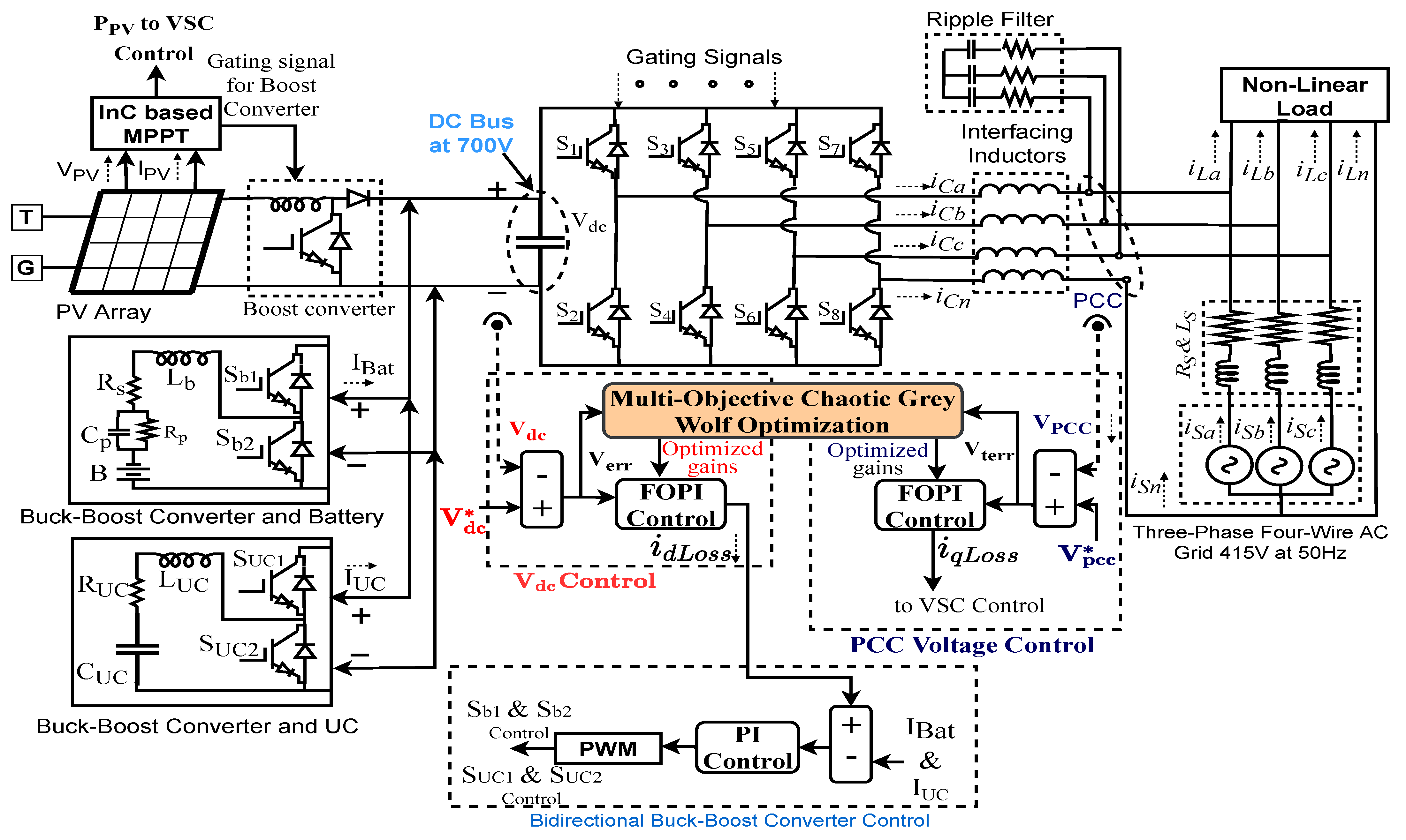
2. System Description

Figure 1 shows the topology of the proposed system. The presented system is a three-phase four-wire (3P-4W) grid-tied PV-HESS. The PV array of 32 kW is connected to the DC bus via a DC-DC boost converter to stabilize PV voltage ( V P V ) during irradiation variation. The MPPT is achieved by using the incremental conductance (InC) method. The HESS involving battery and UC is also attached to the DC bus via a bidirectional DC-DC buck-boost converter to control the charging and discharging operation.
The V d c and V p c c are controlled by multi-objective CGWO (MOCGWO) tuned FOPI controller to minimize their variations during dynamic conditions. The FOPI managed DC bus generates precise i L o s s , which acts as a reference signal for battery current control, suppresses the second-harmonics component at DC bus, and improves the power quality of the system. The two-level VSC is attached to the PCC via interfacing inductors to reduce the voltage and current ripples. The grid at 415 V, 50 Hz is also linked to the PCC. The VSC control is provided by the VSS-ILMS algorithm, which generates the direct and quadrature fundamental component of load current to generate the required reference currents and eliminates the dc offset at PCC. The proposed system is termed smart due to its capability in operating in three modes, i.e., (1). The total power is delivered to the grid during PV to grid mode, (2). During PV-DSTATCOM mode, the load is satisfied with both the PV and grid (3). during DSTATCOM mode, the load is satisfied by the grid only due to the unavailability of PV power. The proposed system with low voltage ride-through capability is also analyzed under load unbalancing and deep voltage sag/swell conditions. The two-level VSC is attached to the PCC via interfacing inductors and R–C filters to reduce the current and voltage ripples produced due to VSC switching. The grid at 415 V, 50 Hz is also attached to the PCC.
The primary characteristics of the presented work are as follows.
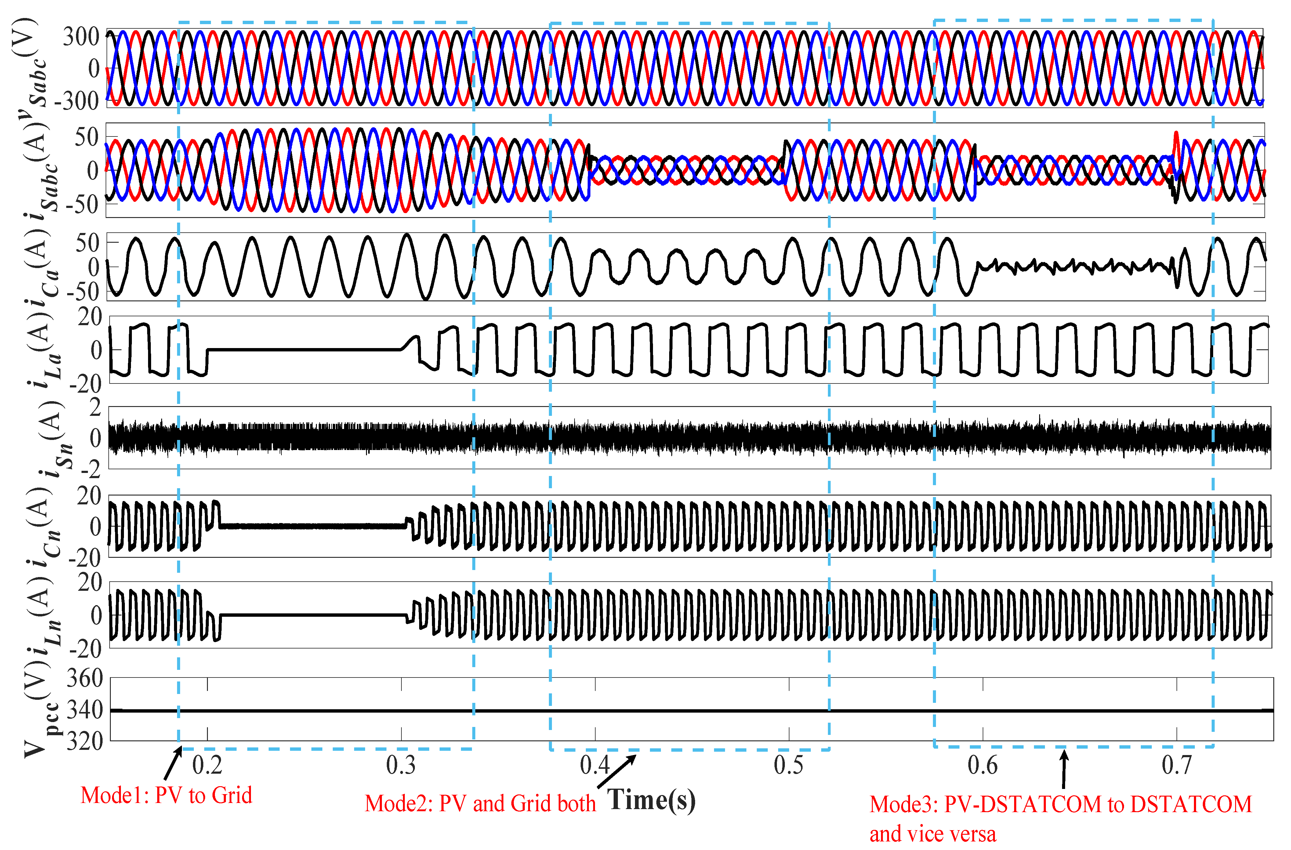
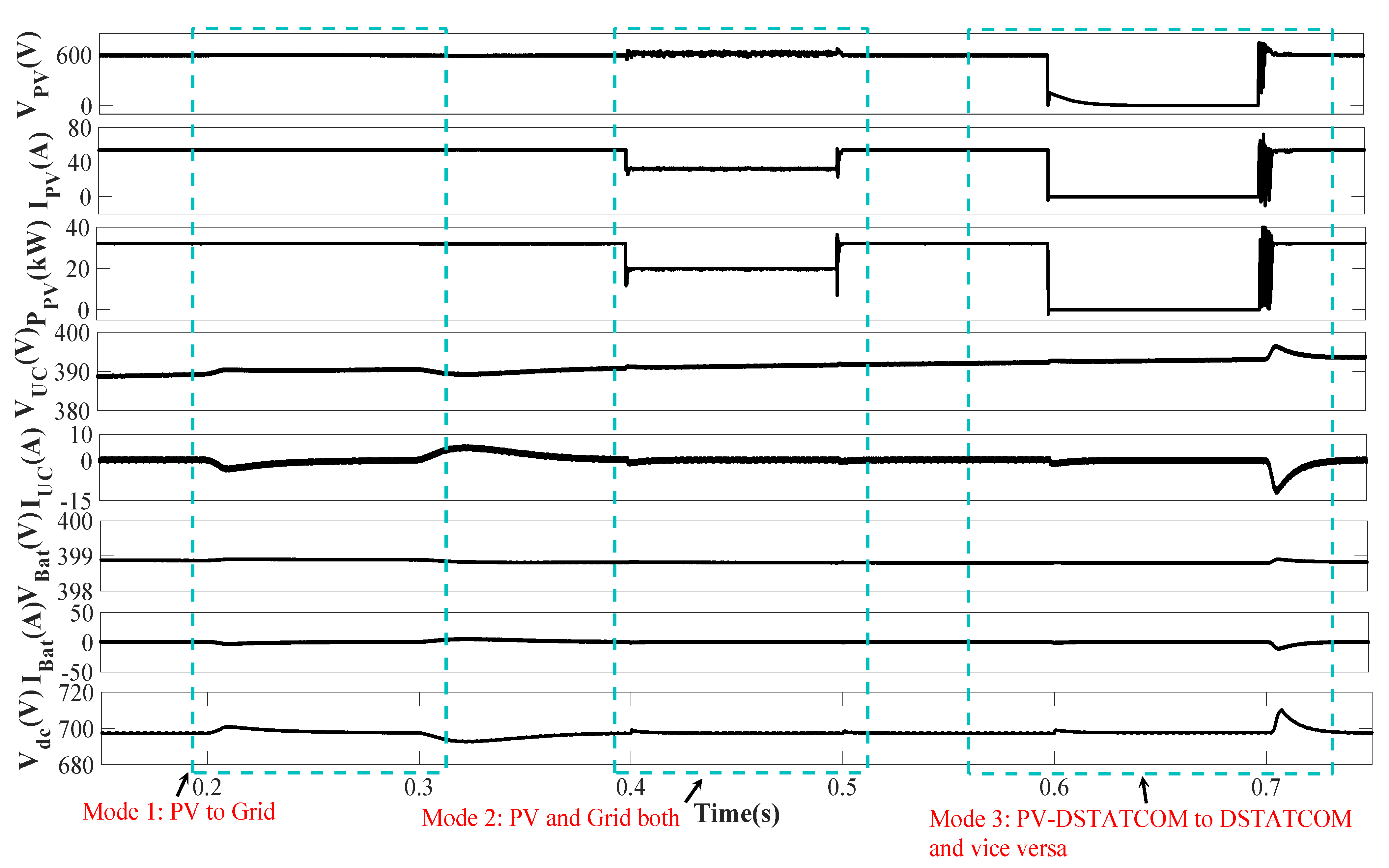
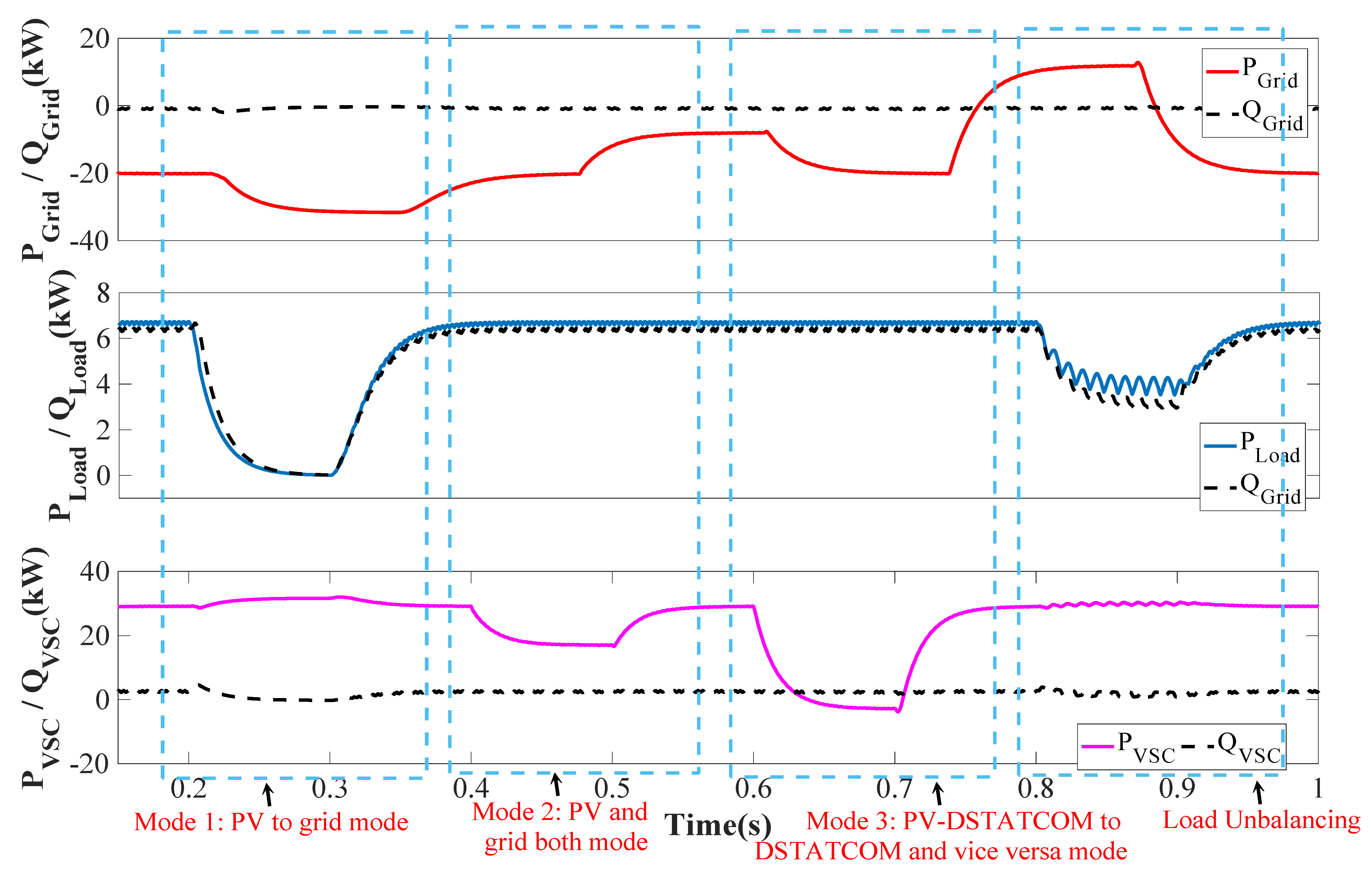
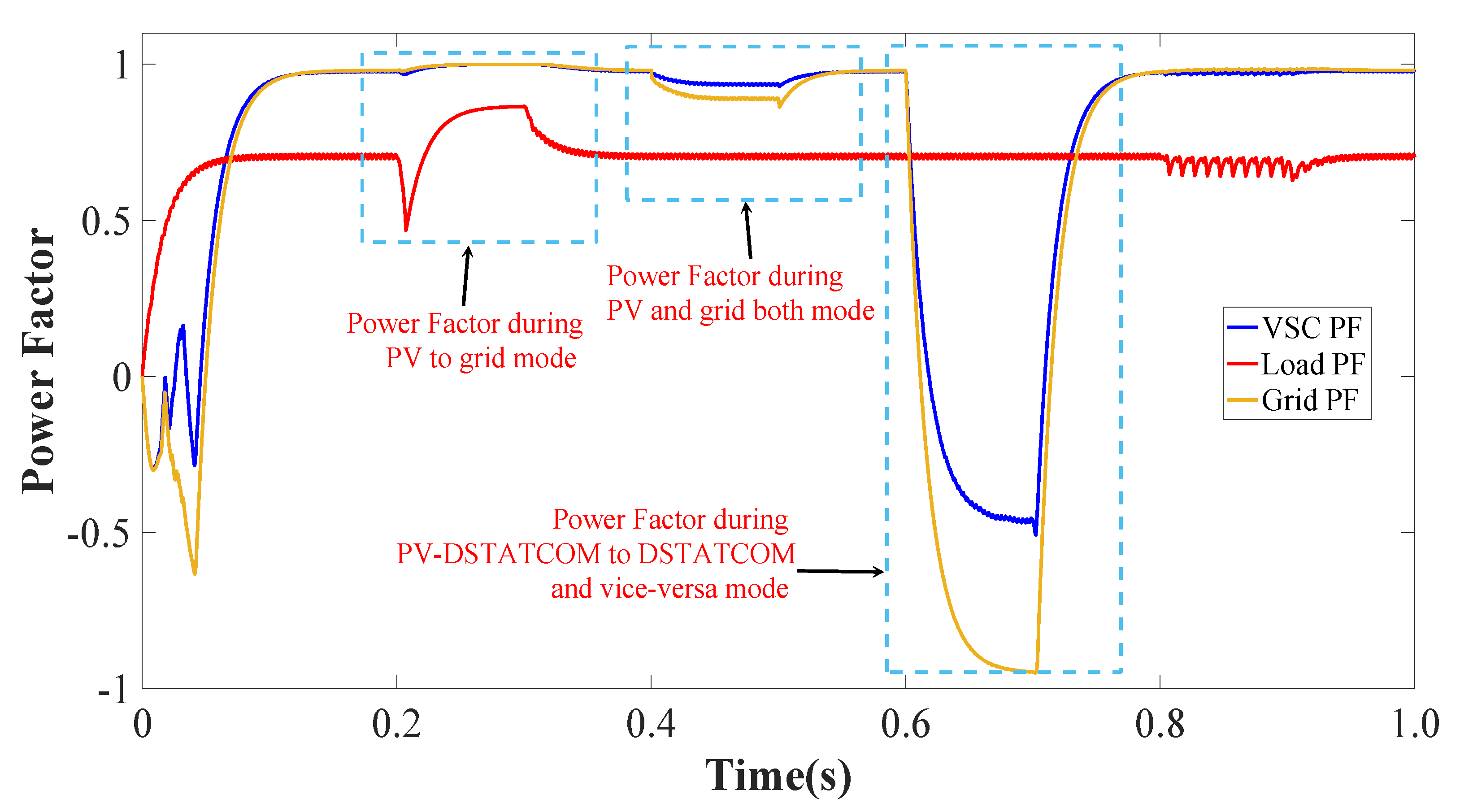
  • Smart grid-tied PV operation: The grid-tied PV system performs satisfactorily in three modes: (1) PV to grid mode, (2) PV-DSTATCOM mode, (3) PV-DSTATCOM to DSTATCOM, and vice versa mode.
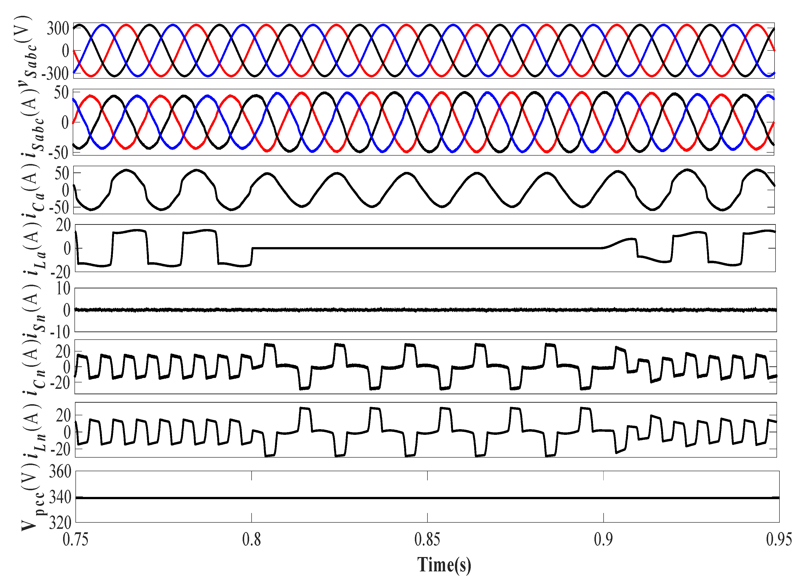
  • Dynamic state operations: The presented system is observed under weak grid conditions like load unbalancing and deep voltage sag/sell condition, i.e., 20%, 40%, and 60%, respectively.
  • Multi-functional operation: The proposed system performs multiple operations, i.e., load balancing, harmonics elimination, active and reactive power control, etc.
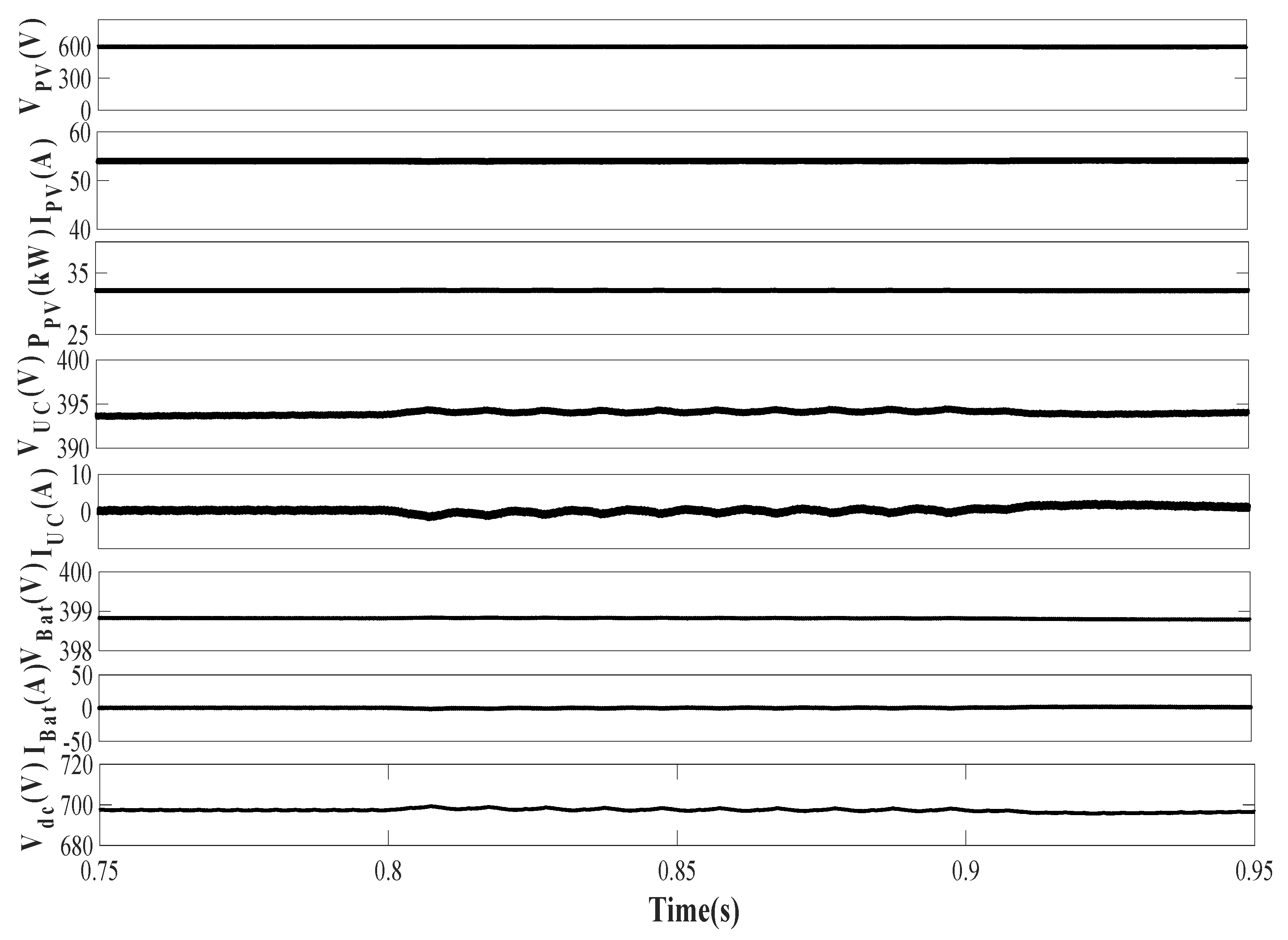
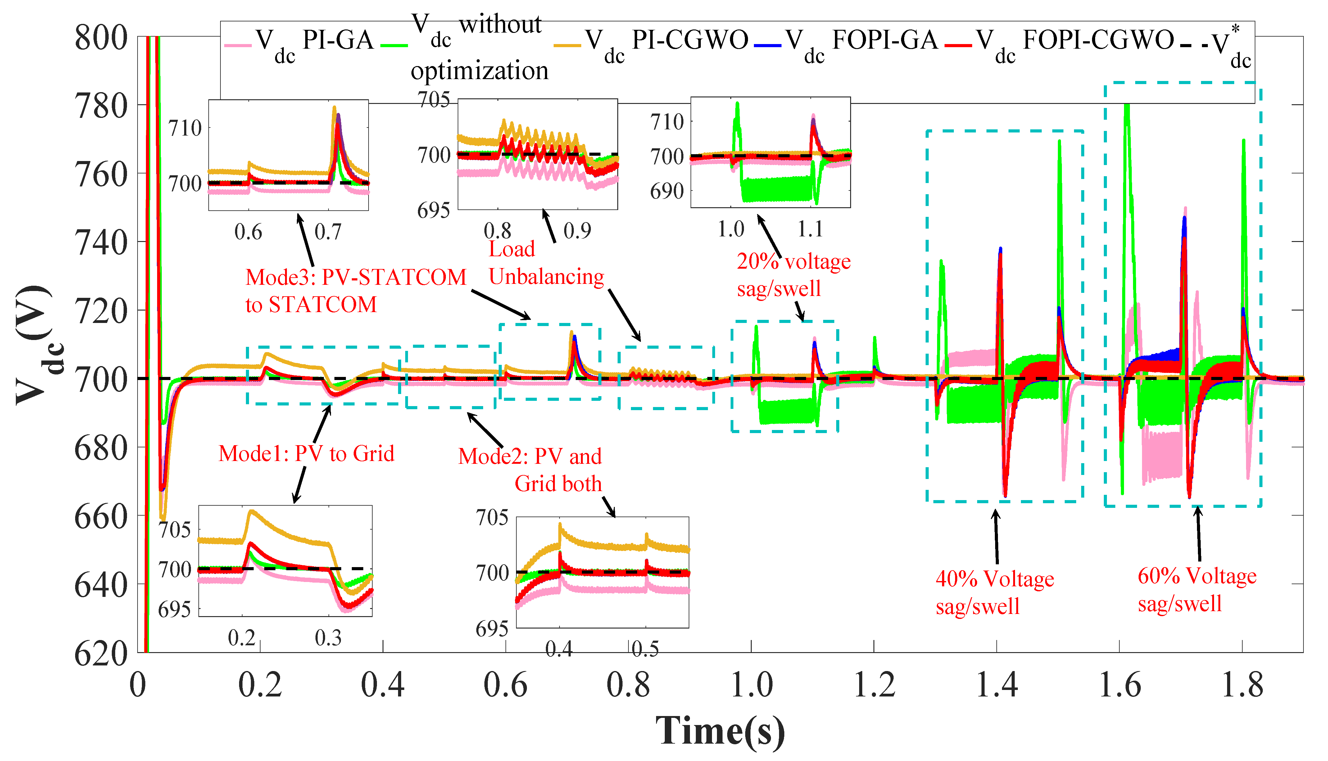
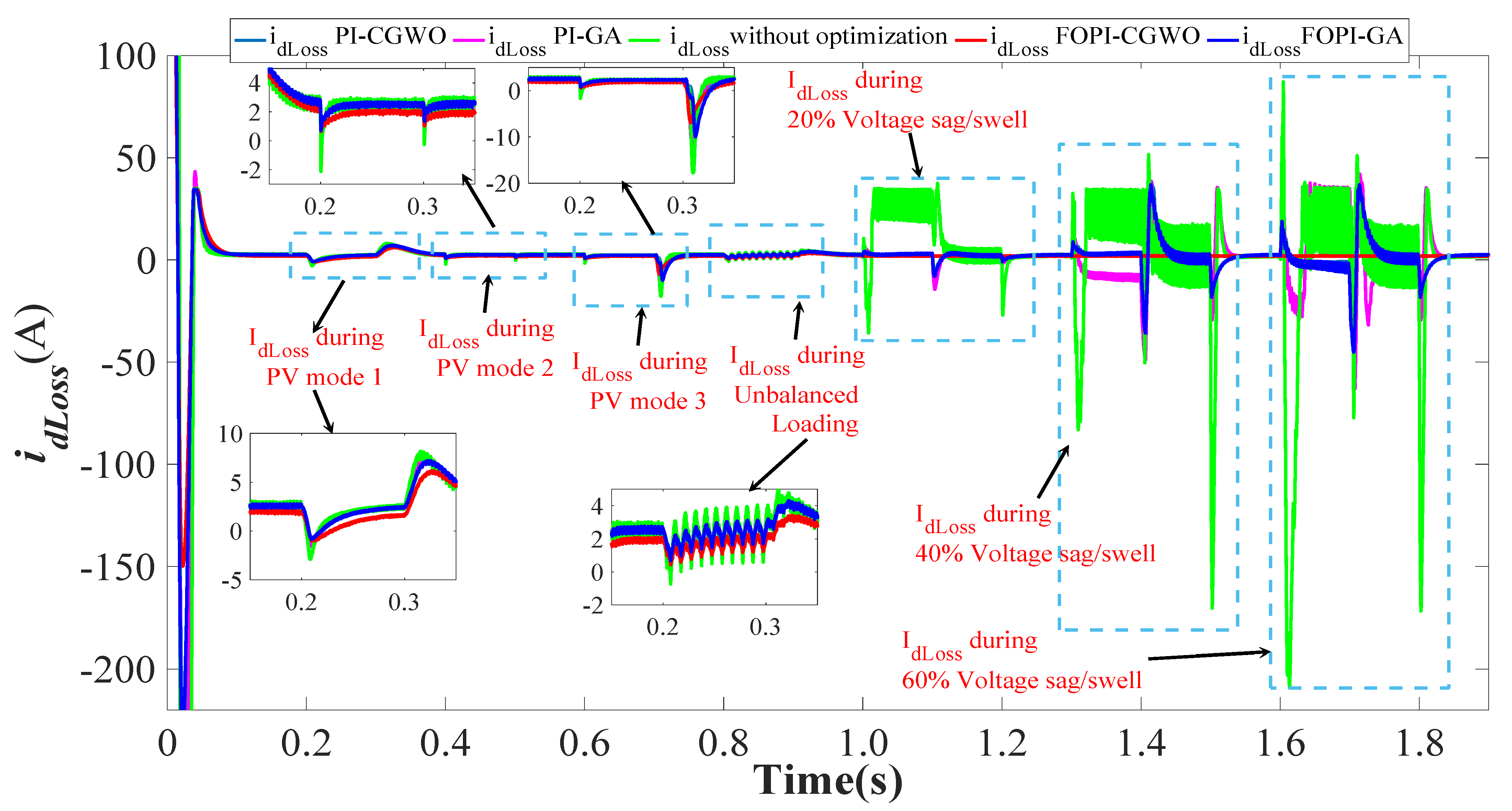
  • DC and AC bus stability performance: The DC and AC bus control is provided by CGWO tuned FOPI controller to stabilize the system during dynamic conditions.
  • HESS: The HESS ensures continuous supply to critical load and enhances the system’s power quality by suppressing the second-harmonics content at the DC bus.

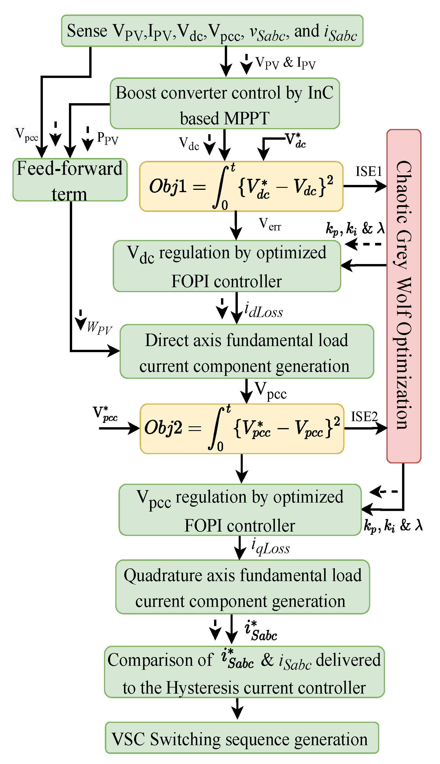
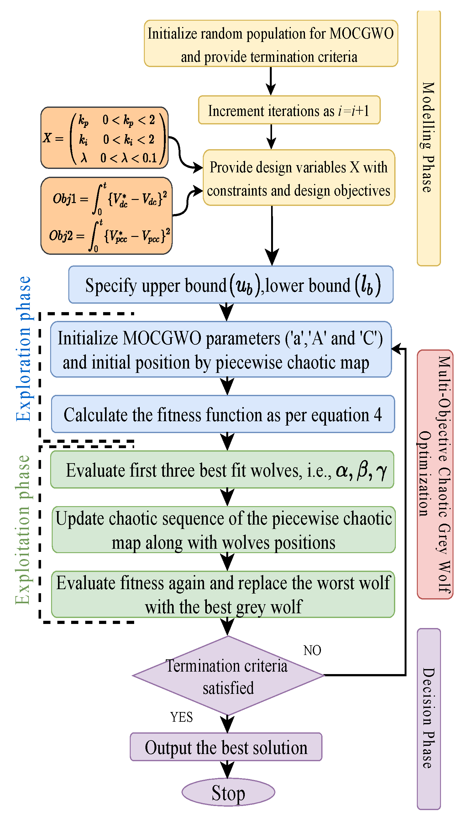
3. Implemented Research Methodology

Figure 2 shows the implemented research methodology of the MOCGWO technique. Various signals, i.e., source voltage ( v S a b c ), source current ( i S a b c ), V p c c , V d c , PV voltage, current, power ( V P V , I P V ,   P P V ) . The V d c and reference V d c , i.e., ( V d c * ) are compared to generate the first objective function (Obj-1), which is an integral square error (ISE-1) as per (1), to be minimized by MOCGWO for delivering optimal gains of FOPI controller, i.e., k p , k i , λ for V d c control. The direct loss component of current ( i d L o s s ) is generated from the V d c control contributes to generating the fundamental elements of load current by VSC control. The V p c c is also compared with the reference V p c c , i.e., ( V p c c * ) to generate a second objective function (Obj-2) with ISE-2 as its error indices as per (2). The Obj-2 minimization also delivers, k p , k i , λ for the V p c c control. The quadrature loss component of current ( i q L o s s ) is further included in the quadrature fundamental component of load current by VSC control. With optimized AC and DC buses, VSC control generates more accurate weight signals and reference currents, which further improves the performance of the proposed system.
Obj - 1 = 0 t ( V d c *     V d c ) 2 = 0 t ( V e r r ) 2
Obj - 2 = 0 t ( V p c c *     V p c c ) 2 = 0 t ( V t e r r ) 2

Multi-Objective Chaotic Grey Wolf Optimization Technique

Figure 3 shows the flowchart of the MOCGWO algorithm, which is inspired by the social hunting behavior of grey wolves. Chaos theory is introduced into the GWO algorithm for accelerating its global convergence speed. Despite having a reasonable convergence rate, GWO has low solving accuracy and poor local searchability. To overcome the shortcomings of GWO, the CGWO algorithm is developed by introducing a piecewise chaotic map in the GWO algorithm to produce a diverse initial population with uniform distribution as per (3). The reader may refer to more information and paradigm [37,38,39,40,41]. The local minima stagnation is avoided by chaos, randomness, and ergodicity.
P k + 1 = { P k 0 p k a p k a 0.5 a a p k 0.5 1 a p k 0.5 a 0.5 p k 1 a 1 p k a 1 a p k 1 }
The exact hierarchy of wolves in a wolf pack is considered as GWO, which is α , β , γ , and ζ . The roles and responsibilities of wolves in the group reduce with the descending order. The α wolf is a pack leader, responsible for giving instructions and decision making. β wolf is second in command and the best candidate to replace α . γ wolves take order from α , β and dominate ζ , which is fourth and the last level. ζ wolves maintain safety and integrity in the wolf pack.
This first step of MOCGWO is to generate a diverse population with uniform distribution initialization of wolf pack. The chaotic map described in (3) is mapped with the iterative algorithm to initialize the first chaotic numbers. Various parameters involved in the CGWO algorithm for conducting exploration-exploitation mechanism viz. ‘a’, ‘A’ and ‘C’ are generated, the same as in GWO (4)–(6). The distances from α , β , and γ wolves, i.e., D α , D β , and D γ to each of the remaining wolves ( p ) as a fitness function, using which the effect of α , β and γ wolves on the prey viz. p 1 , p 2 , and p 3 can be calculated further. The fitness of an initialized population of the wolf in search space is calculated and sorted using the introduced chaotic map and are sorted according to their fitness. The fittest wolf position will be updated in the next iteration (7) and may get the wolf’s position as the optimal solution in case termination criteria are fulfilled. In each iteration, associated parameter values are also updated (6). With termination, criteria satisfied the leader wolf’s fitness or position will be considered the most optimal solution or PI controller gains for V d c and V p c c regulation by the MOCGWO algorithm.
D α = | C 1 × p α p | ,   D β = | C 2 × p β p | ,   D γ = | C 3 × p γ p |
p 1 = p α A 1 × D α , p 2 = p β A 2 × D β , p 3 = p γ A 3 × D γ
A = 2 a × r 1 a ,   C = 2 × r 2
p ( t + 1 ) = ( p 1 + p 2 + p 3 ) / 3

4. Controlling Strategies

The proposed system is controlled by mainly three controls, which are (1) Incremental conductance (InC) based MPPT control. (2) DC bus and HESS current control and (3) VSS-ILMS based VSC control.

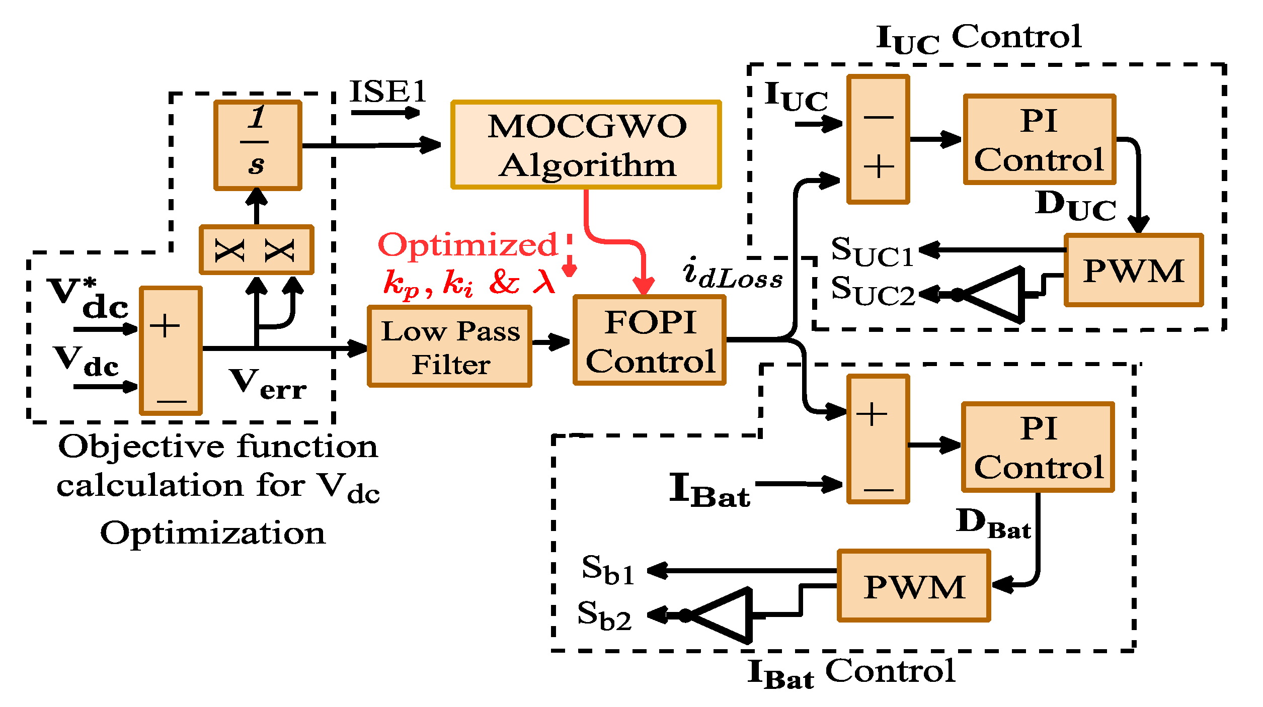
4.1. DC Bus Voltage and HESS Current Control

Figure 4 shows V d c control along with HESS current control. The DC bus is controlled by a FOPI controller, which receives its optimized gains from the MOCGWO technique to minimize the V d c variation during dynamic conditions. The i d L o s s acts as a reference signal for battery and UC current control or charging/discharging control. The optimized i d L o s s will be smoother and free from sharp edges, which reduces the stress on the HESS, increasing the storage system’s longevity.

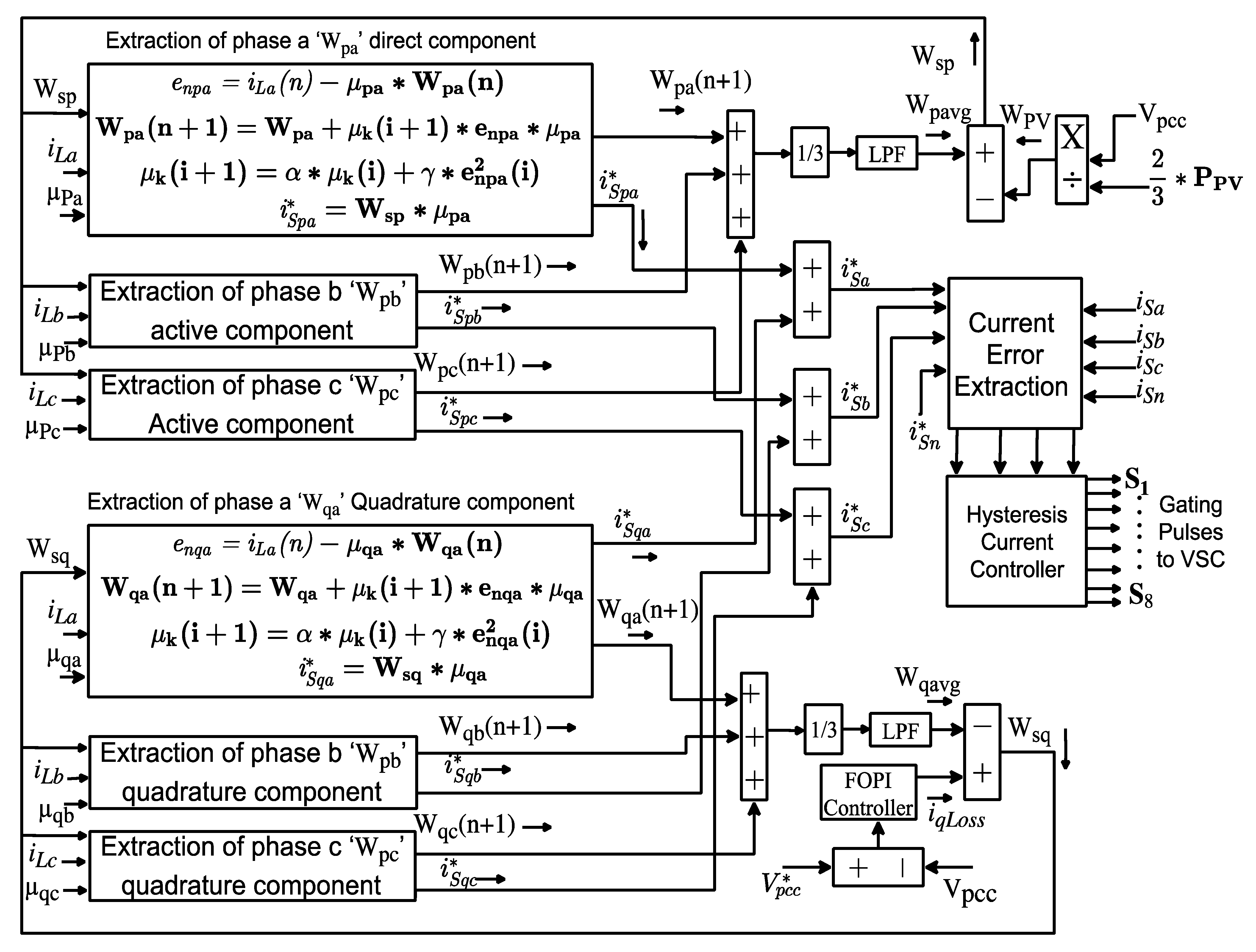
4.2. Voltage Source Converter Control

Figure 5 shows the VSS-ILMS based VSC control. The proposed control with incremental variable step-size reduces steady-state error and faster convergence speed. With every iteration, the step-size increases, which can filter a wide variety of noises without increasing the computational burden. The network approximation with the proposed control is easy, performing better with the sparse network. This gradient-based VSC control reduces the mean square error (MSE) out of the load current component. The optimized DC and AC bus components help VSC control generate the accurate weight components and reference current signals, which further improves the VSC performance.
For the direct weight components generation ( W P x , where x = a, b, c), error signals ( e n x , where x = a, b, c) for each phase are produced as per (8) as a function of the i L a b c and the in-phase component ( μ p x ) . The μ p x , x = a, b, c, are calculated as per (9), V p c c is voltage magnitude and v s x , where x = a, b, c, are the phase to ground source voltages [15].
e n x = i L x ( n ) μ p x × W p x ( n ) ,   where   x = a ,   b ,   c
μ p x = v s x V p c c = v s x 2 3 ( v s a 2 + v s b 2 + v s c 2 ) ,   where   x = a ,   b ,   c
The W P x , where x = a, b, c are calculated for each phase as a function of the error signal and incremental step-size ( μ k ( i + 1 ) ) as per (10) and (11).
W p x ( n + 1 ) = W p x ( n ) + μ k ( i + 1 ) × μ p x × e n p x ;   where   x = a ,   b ,   c
μ k ( i + 1 ) = α × μ k ( i ) + γ × e n p a 2 ( i )
The overall direct weight signal ( W s p ) is calculated as a function of average weight components ( W p a v g ) and feed-forward term ( W P V ) as per (12)–(15).
W P V = 2 3 ( P P V 2 3 ( v s a 2 + v s b 2 + v s c 2 ) ) = 2 3 P P V V p c c
W p a v g = 1 3 ( W p a + W p b + W p c )
W s p = W p a v g W P V
i spx * = W sp × μ p x   where   x = a ,   b ,   c
For the quadrature weight component generation ( W q x , where x = a, b, c), error signals ( e n q x , where x = a, b, c) are calculated as per (16). The quadrature-phase components ( μ q x ,   where , x = a, b, c) is calculated as a function of in-phase components as per (17).
e n x = i L x ( n ) μ p x × W p x ( n ) ,   where   x = a ,   b ,   c
μ q a = μ p a + μ p c 3 ;   μ q b = 3 μ p a 2 + μ p b μ p c 2 3 ;   μ q c = 3 μ p a 2 + μ p b μ p c 2 3
The W q x , where x = a, b, c are calculated for each phase as a function of the error signal and incremental step-size ( μ k ( i + 1 ) ) as per (18) and (19).
W q x ( n + 1 ) = W q x ( n ) + μ k ( i + 1 ) × μ q x × e n q x ;   where   x = a ,   b ,   c
μ k ( i + 1 ) = α × μ k ( i ) + γ × e n q a 2 ( i )
The overall direct weight signal ( W s q ) is calculated as a function of average weight components ( W q a v g ) and i q L o s s as per (20)–(22).
W q a v g = 1 3 ( W q a + W q b + W q c )
W s q = W q a v g i q L o s s
i sqx * = W sq × μ q x   where   x = a ,   b ,   c
The overall reference current ( i sx * , where x = a, b, c) is generated by doing the sum of i sdx *   and   i sqx * as per (23).
i sx * = i sdx * + i sqx *   where   x = a ,   b ,   c
The i s x * , where x = a, b, c are delivered to the hysteresis current controller (HCC) for VSC switching signal generation.

5. Results and Discussion

The presented system is observed and analyzed under various dynamic conditions, including three modes of smart PV operation, shallow to deep voltage sag/swell, and load unbalancing. The following results and discussion validate the performance of the system.

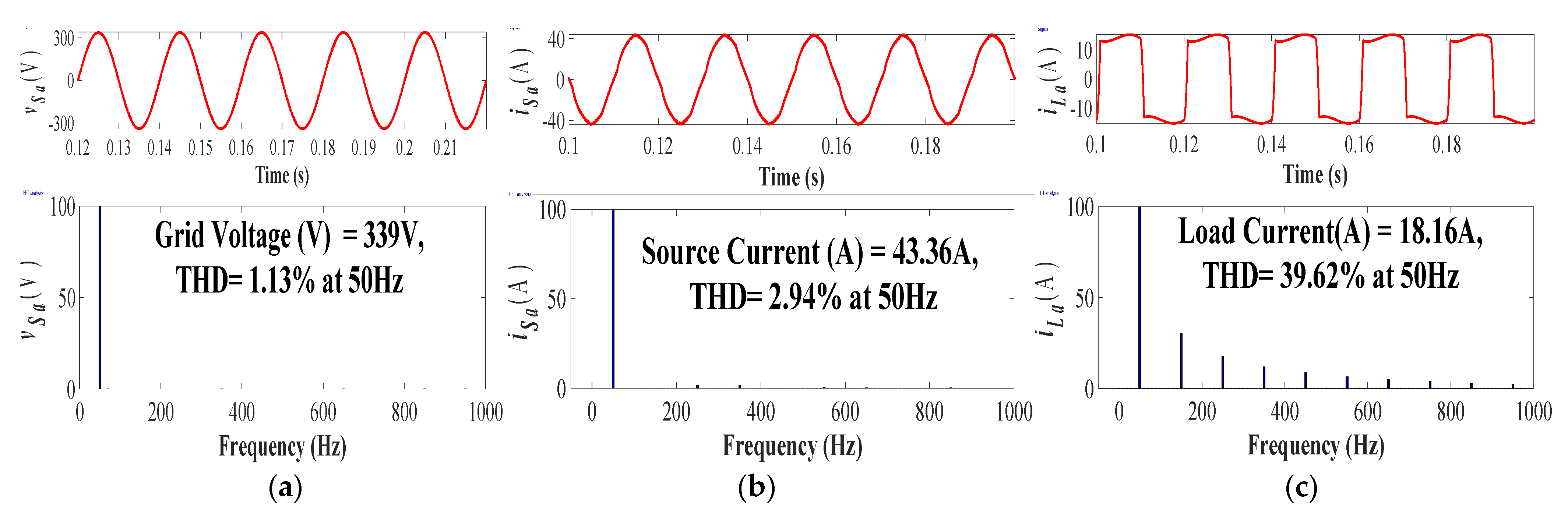
5.1. Steady-State Analysis

Figure 6a–c presents the steady-state analysis of phase ‘a’ of source voltage ( v S a ), source current ( i S a ) and load current ( i L a ). During steady-state, the solar irradiation level was kept fixed at 1000 W/m2. The THD level of grid voltage and current were maintained well within the 5% limit as per IEEE 519 standards. In the proposed system, AC and DC bus control was provided by PI and FOPI controllers. The PI and FOPI controllers were supplied with GA and CGWO optimized for better performance. Table 2 shows the grid THD levels with diverse controllers implemented. The CGWO tuned FOPI controller delivered the lowest THD level during steady-state.
The VSC control of the above-described system was also compared with the other adaptive controls to prove the better filtering capability of the implemented VSS-ILMS control. Table 3 shows the THD performance of the grid with LMS, LMF, and VSS-ILMS control. For this analysis, AC and DC buses were regulated by CGWO tuned FOPI controller.

5.2. Smart Grid-Tied PV System Performance Analysis

The presented system is termed a smart grid-tied PV system as it can operate in three different modes and effortlessly shifts from one mode to another.
During mode-1, the grid-tied PV system does not deliver any power to the local load; in contrast, the grid itself absorbs the full PV power.
During mode-2, the grid and PV system both satisfy the load requirements; if the load demand is less than PV power generation, the remaining power will be delivered to the grid. If the irradiation level reduces, the HESS and grid provide the remaining required power.
During mode-3, in sunshine conditions, the grid-tied PV system operates as a PV-DSTATCOM, whereas during bad weather conditions or nighttime, the proposed system shifts to DSTATCOM mode. In DSTATCOM mode, load requirements are fulfilled by the grid only. When PV power becomes available, the system shifts to PV-DSTATCOM mode effortlessly without any transients.
The presented system was analyzed under each mode of PV operation. Figure 7 shows the three smart PV operational mode analysis by associated AC quantities, i.e., v S a b c ,   i S a b c , phase ‘a’ compensator and load current ( i C a   and   i L a ) , neutral current of source, compensator, and load ( i S n , i C n , i L n ) and V p c c .
Mode-1 operation was executed from 0.2 s to 0.3 s, where no load was connected to the system, and whole power was delivered to the grid. The v S a b c and i S a b c maintained the out of phase relation, as power was provided to the grid. The i S a b c magnitude increased as more power was available without the local load. The i L a and i L n also remained zero in the absence of the load. The compensator neutral current remained in phase opposition of i L n to maintain the i S n = 0 , in this case i L n is already zero, hence i C n is also remained zero as well i S n . The V p c c was maintained at the desired level.
Mode-2 operation was executed from 0.4 s to 0.5 s, where the irradiation level was reduced from 1000 W/m2 to 600 W/m2 to confirm the combined operation of the grid and PV system. With reduced irradiation level, the power delivered to the grid reduces, hence, i S a b c also. Though v S a b c and i S a b c remained in phase opposition as PV power at the reduced insolation level was sufficient for load requirements. The i C n and i L n were in phase opposition, canceling out each other at three times the fundamental frequency. The i S n was maintained near zero, hence confirming the neutral current compensation.
Mode-3 is executed from 0.6 s to 0.7 s, during which the irradiation level is reduced to zero. In the absence of PV power system shifts from PV-DSTATCOM to DSTATCOM operation. At 0.6 s, the phase reversal of i S a b c was observed, earlier v S a b c and i S a b c were in phase opposition, but after 0.6 s, both came in phase with each other, confirming the power supply from the grid to load. After 0.7 s, the irradiation level was again increased to 1000 W/m2, due to which the system shifted from DSTATCOM to PV-DSTATCOM operation. The V p c c magnitude was maintained at the desired level with the help of AC bus voltage control.
Figure 8 shows the behavior of DC quantities during smart PV operations. The PV voltage, current, and power ( V P V , I P V and P P V ), battery and UC voltages and currents ( V B a t , I B a t , V U C , I U C ) and DC bus voltage V D C are shown as DC quantities of the system.
During Mode-1: The irradiation level is maintained at 1000 W/m2, where whole power was delivered to the grid. The battery and UC start charging during mode-1, I B a t and I U C   became slightly negative and, V B a t and V U C   started increasing. The V d c was maintained at the desired of 700 V during PV to grid operation.
During mode-2: the irradiation level was reduced from 1000 W/m2 to 600 W/m2. The V P V was kept at the fixed voltage level of 600 V, whereas I P V and P P V changed with the reduced irradiation level. During this mode, both PV and the grid manage the load demand. The V d c was maintained at the desired level.
During mode-3, the solar irradiation level reduced from 1000 W/m2 to 0 W/m2 resulting in the proposed system shifting from PV-DSTATCOM to DSTATCOM operation. The V P V , I P V , and P P V became zero to simulate the absence of sunshine. The grid itself and HESS charges managed the load slowly from the grid power. After 0.7 s system shifts from DSTATCOM to PV-DSTATCOM operation without any significant transient on load and grid side of the system. The V d c was maintained at the desired level of 700 V, as shown in Figure 8.
Figure 9 shows the active and reactive power flow of the grid side ( P G r i d , Q G r i d ), load side ( P L o a d , Q L o a d ) and compensator side ( P V S C , Q V S C ) during three modes of smart PV operations. The reactive power delivered by the grid ( Q G r i d ) remained almost zero throughout the smart PV operation as VSC gives the necessary reactive power to load, keeping the reactive power exchange with grid minimum. The grid active power exchange ( P G r i d ) changed with the mode of operation. During PV to grid mode, P G r i d became negative as the grid absorbed the active power. The load demand of active and reactive power became zero as the load was disconnected during this mode. The compensator was converting DC power to AC power and delivering to the grid, so the P V S C , Q V S C was the same as P G r i d , Q G r i d during mode-1.
During mode two operation, the P L o a d , Q L o a d remained fixed. The P V S C changes with the change in irradiation level and the same power were provided to the grid as P G r i d .
During mode three operation, the PV power became zero in the DSTATCOM operation; the load demand remained fixed during this mode also. The P V S C became negative to support the changing of HESS and P G r i d was delivered to the load.
Figure 10 shows the power factor (PF) variations during smart PV operation. The VSC control operated in zero voltage regulation mode, where it aimed to manage voltage at PCC and compensate reactive power. The load PF remained around 0.8 p.u. during smart PV operation and load unbalancing, which changed slightly with the connection and disconnection of load during PV to grid mode. Both VSC and grid PFs have the same behavior. During PV-DSTATCOM mode, the grid PF reached –1 due to the reversal of flow of power, and the earlier grid was absorbing, and then the grid was supplying.

5.3. Load Unbalanced Analysis

Figure 11 shows the load unbalancing analysis created by disconnecting the phase ‘a’ of the load from the system. During load unbalancing, i L a became zero, i S a magnitude increased slightly as only two phases of load, around 66%, needed to be managed, and the remaining was delivered to the grid. The i L n and i C n cancelled each other at twice the fundamental frequency, hence maintaining the i S n = 0 . The V p c c was kept at 339 V.
On the DC side, V P V , I P V and P P V showed no change and kept following their references as irradiation level was kept fixed at 1000 W/m2. The I B A T and I U C charging rate increased slightly. The DC bus stability was preserved, and V D C was maintained at 700 V while following the V d c * . As shown in Figure 12. The PF and grid, load, and VSC power are demonstrated in Figure 9 and Figure 10.

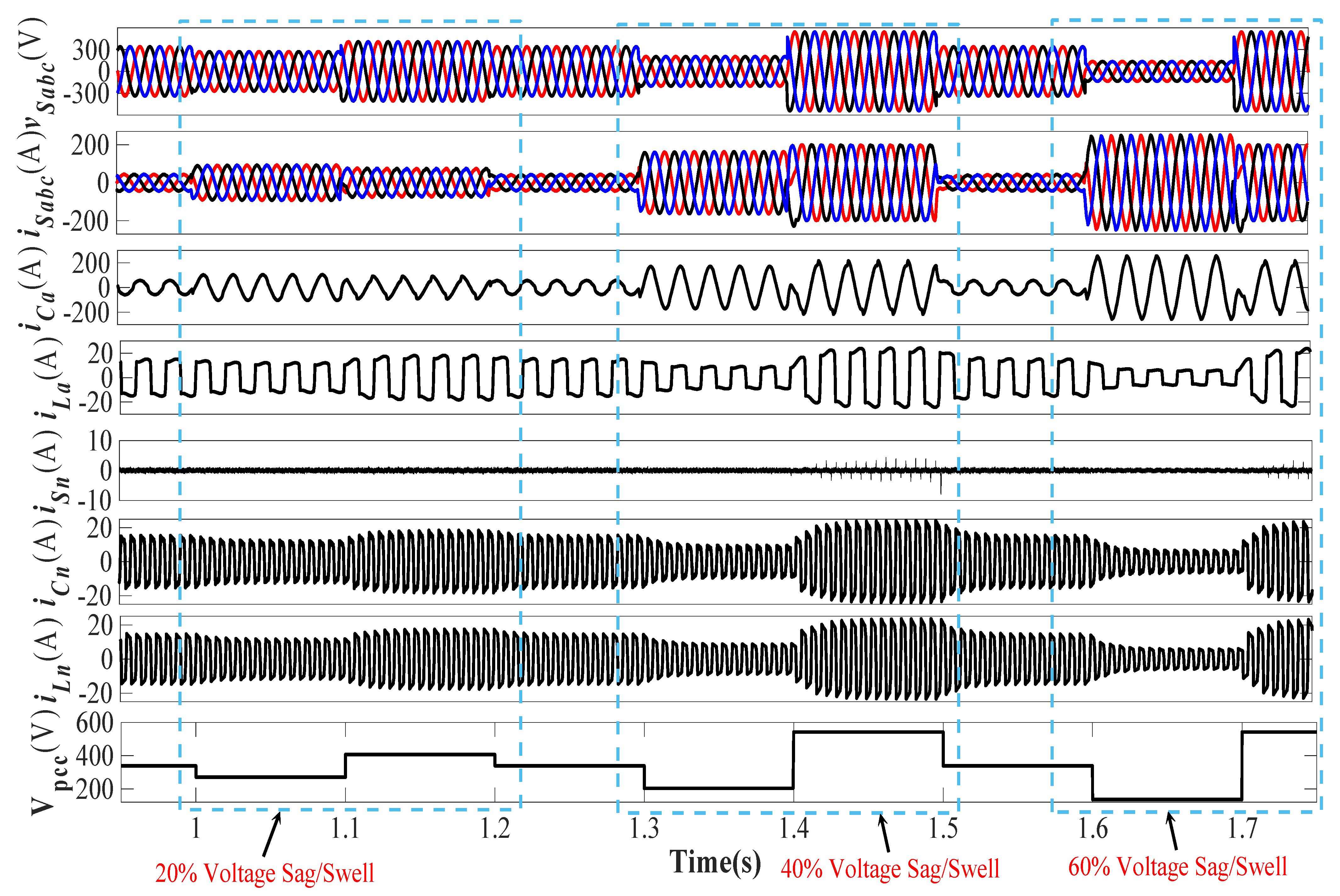
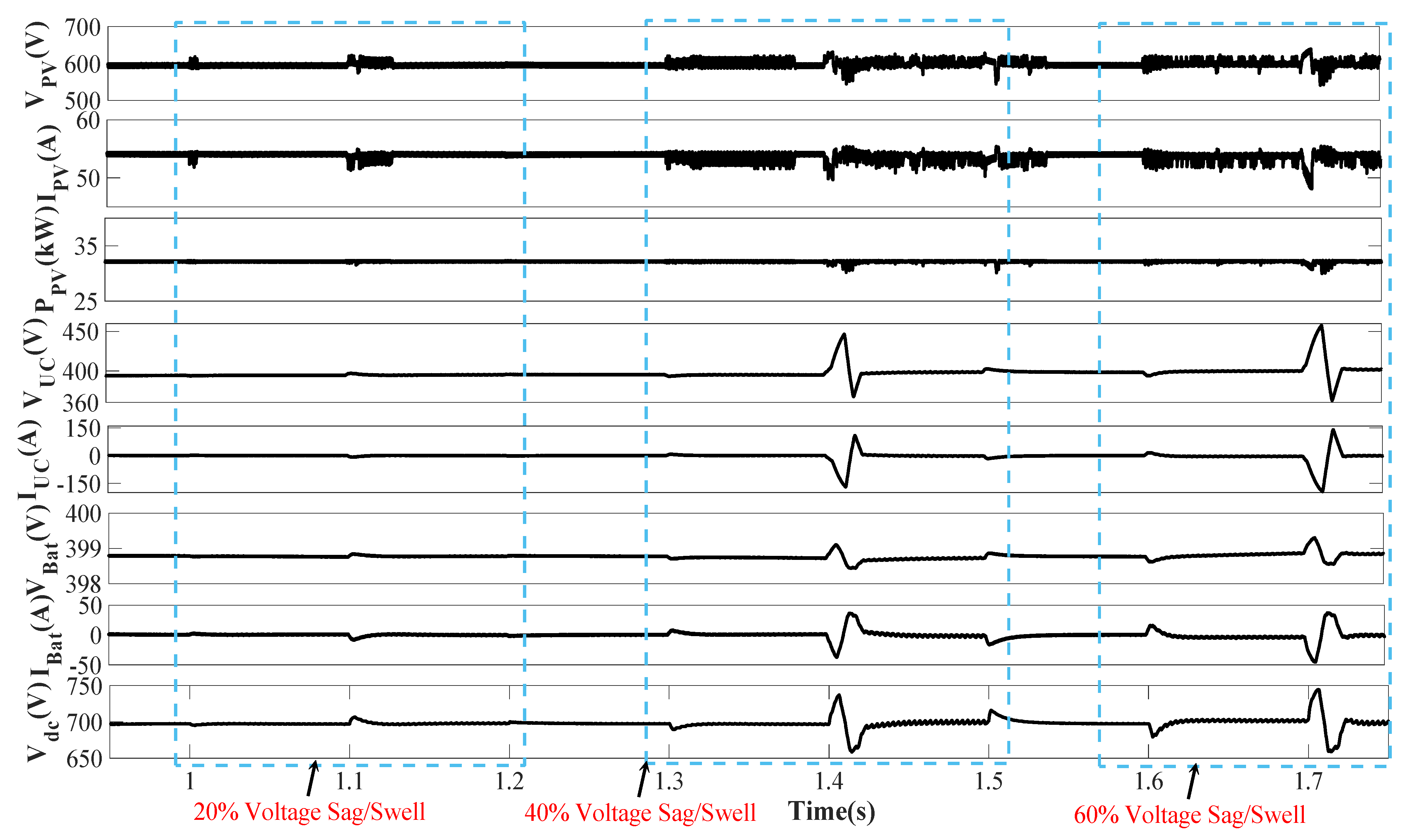
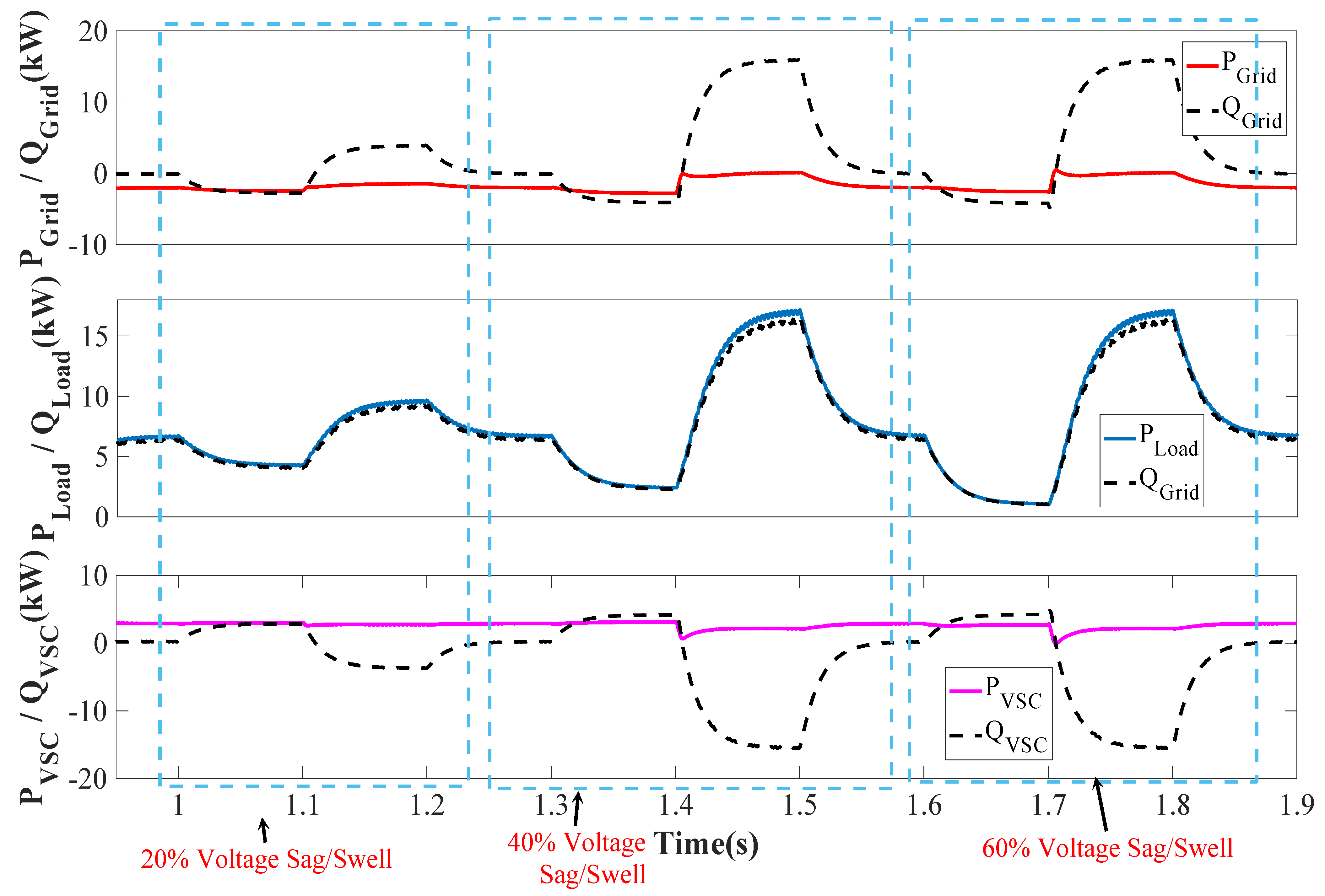
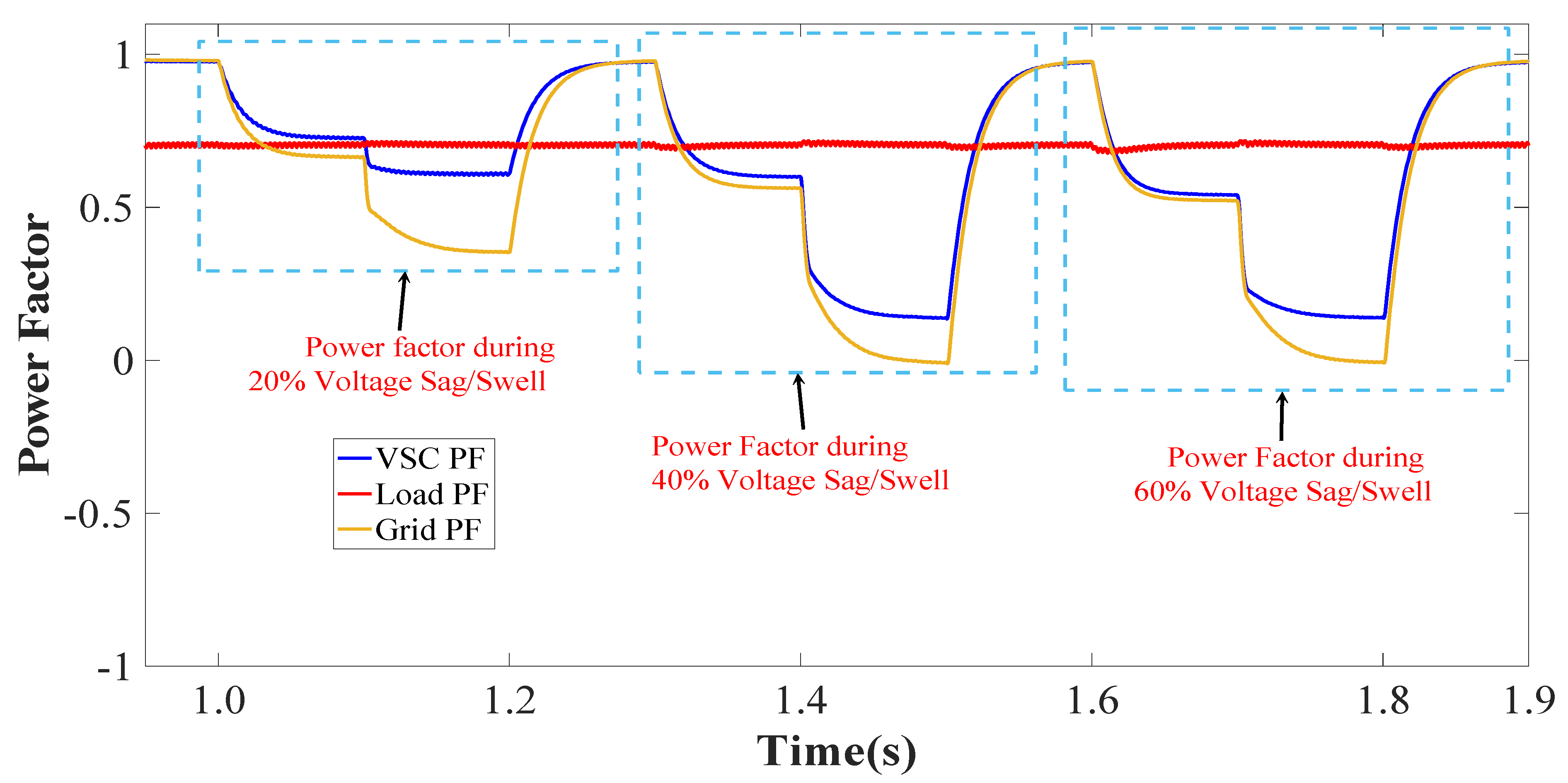
5.4. Abnormal Grid Voltage Analysis

The grid voltage sag and swell are created by varying the three-phase voltage magnitude. The system was analyzed from shallow sag/swell of 20% to deep sag/swell of 60%. Figure 13 shows the performance of AC quantities during abnormal grid voltages.
The grid voltage sag/swell of 20% was created from 1.0 to 1.2 s, the i S a b c remained sinusoidal, and its magnitude increased with voltage sag and reduced with the swell. The magnitude of i C a , i L a , i C n , i L n also changed with the variation in grid voltage. The V p c c waveform also confirms the occurred sag/swell.
During 40% of voltage sag/swell, the variations in currents magnitude are higher, but the i S a b c maintained its sinusoidal nature. The i S n was maintained at zero, confirming the neutral current compensation.
During 60% grid voltage sag swell, the magnitude of various currents signals rose while maintaining the system’s stability. During deep voltage sag/swell, PV remained connected to the system with low ride-through capability. The VSC control retained the sinusoidal nature of source current during these weak grid conditions, vouching for the efficient control algorithm.
Figure 14 shows the performance of DC quantities during abnormal grid voltages. The V P V , I P V , P P V remained almost the same during voltage sag/swell conditions, other than swell variations in deep voltage sag/swell conditions. During the transition from sag to swell mode, battery and UC currents show significant variations but quickly adjusted to new conditions. The battery system was supported with the current control mechanism, whereas UC does not require high current protection, so the variation in I U C was higher than I B a t . The DC bus is crucial for the system’s stability; during deep voltage sag/swell the V d c variations were not very significant. The FOPI-based V d c control along with VSC control stabilized the DC bus quickly and did not allow a huge deviation from the reference point during extremely weak grid conditions.
Figure 15 shows the grid, load, and VSC active and reactive power performance during abnormal grid voltage conditions (extreme weak grid conditions). With grid voltage abnormalities, load active and reactive power requirements increased sharply. During deep voltage, sag/swells reactive power demand increases rapidly, collectively managed by the grid and VSC to maintain the healthy operation.
Figure 16 shows the PF variations of load, grid, and VSC side. The load weak grid PF remained the same throughout the operation. With voltage sag and swell conditions, the PF adjusted itself to new values depending on the phase variation with source currents. The VSC PF complements the grid PF, but during deep voltage, sag/swell conditions PF decreased to a shallow level confirming the growing demand for reactive power during extreme weak grid conditions.

5.5. DC and AC Bus Stability Analysis

The DC bus stability is crucial for the stability of the grid-tied PV system. As DC bus controls the flow of power from PV and HESS. The grid voltage itself assists the AC bus voltage control in the grid following converters. The optimized DC and AC bus generate an accurate direct and quadrature loss component of currents ( i d L o s s   &   i q L o s s ). These loss components help the VSC control generate accurate weights and reference current signals. The VSC control with optimized AC and DC busses performs better in harmonics elimination and overall losses reduction.
Figure 17 shows the V d c variations during diverse, dynamic conditions considered. The CGWO tuned FOPI controller performed effectively in reducing the V d c variations. With the implemented DC bus control, the presented system maintains its stability during extreme weak grid conditions, i.e., PV-DSTATCOM to STATCOM and vice-versa, in deep voltage sag swell conditions.
Figure 18 shows the variations of i d L o s s during induced dynamic conditions. In ideal conditions i d L o s s should be zero, with the help of CGWO tuned FOPI controller, presented system minimizes its variations. Even during the sag/swell conditions with FOPI control the i d L o s s is maintained near-zero without significant sharp edges.
The AC bus voltage control in a grid-following converter is partially controlled by the grid voltage also. The AC bus voltage magnitude control with CGWO and GA tuned PI, and FOPI controller is observed. All of the AC bus controls maintain the V p c c at the desired level, and CGWO based FOPI control maintains the V p c c at the desired level as well maintains the i q L o s s component near zero. Table 4 presents the analytical performance analysis of V d c with CGWO and GA optimized FOPI and PI controllers.

5.6. THD Performance Analysis during Dynamic Conditions

Table 5 describes the THD analysis of v S a , i S a , and i L a during diverse conditions. The table also presents the THD comparison of CGWO-FOPI control with other implemented controls for AC and DC bus voltage control.

6. Conclusions

This paper describes a FOPI VSS-ILMS based VSC control of a three-phase four-wire grid-tied PV-HESS system. The DC and AC buses are regulated by the chaotic grey wolf optimized FOPI controller to reduce V d c and V p c c voltage variation during induced dynamic conditions. The DC bus controls the active power flow from PV and HESS to the grid and load, along with the flow of power, which makes the DC bus control crucial for maintaining the overall system’s stability during steady and dynamic states. The optimized DC bus eliminates the second-harmonics component on the DC coupling capacitor, resulting in enhanced power quality. On the other hand, in the case of grid-following inverters, the AC bus voltage is partially controlled by the grid itself. Implementing different controls for the AC bus regulation will have a minute impact on overall system performance. The AC bus control helps to achieve desired reactive power flow while operating under zero voltage regulation mode. Both optimized AC and DC buses produce direct and quadrature loss components of currents, which further enhance the VSC control performance by generating accurate weight signals and reference current signals. The VSC control suppresses the dc offset at PCC, which improves the system’s performance. The VSS-ILMS algorithm controls the VSC, which increases the step size in each iteration to accommodate a wide variety of noise signals to be passed through the filtering window. The network approximation with proposed gradient-based adaptive control is easy, performing better with the sparse network. The proposed control provides VSC with the capability to perform a multi-functional operation while ensuring the system’s stability. The proposed system performs active and reactive power control, neutral current compensation, load balancing, harmonics elimination, etc., during the diverse, dynamic, and extremely weak grid conditions. Due to the offset rejection capability of the VSC and optimized DC and AC buses, the system remains stable up to 60% voltage sag/swell conditions. The THD of the attached distribution grid voltage is merely 1.13% and the current is 2.94% during steady-state. Even during dynamic conditions, the THD level is well maintained with 5%, even during dynamic conditions, i.e., PV to grid mode, load unbalancing and deep voltage sag/swell conditions. The CGWO tuned DC bus minimize the deviation of V d c from its reference. The steady-state deviation of V d c is hardly 0.57% (≅3 V), however, during 60% voltage sag/swell condition, it varies maximum up to 6.68% ( 45 V), which surely reduces the stress on DC coupling capacitor and VSC switches. The overall performance of the proposed system is found satisfactory as per the IEEE519 standard.

Author Contributions

Conceptualization, M.C., I.H., A.A., H.M. and M.A.A.; methodology, M.C., I.H., A.A., H.M. and M.A.A.; software, M.C., I.H., A.A., H.M. and M.A.A.; validation, M.C., I.H., A.A., H.M. and M.A.A.; formal analysis, M.C., I.H., A.A., H.M. and M.A.A.; investigation, M.C., I.H., A.A., H.M. and M.A.A.; resources, M.C., I.H., A.A., H.M. and M.A.A.; data curation, M.C., I.H., A.A., H.M. and M.A.A.; writing—original draft preparation, M.C., I.H., A.A., H.M. and M.A.A.; writing—review and editing, M.C., I.H., A.A., H.M. and M.A.A.; visualization, M.C., I.H., A.A., H.M. and M.A.A.; supervision, M.A.A.; project administration, H.M. and M.A.A.; funding acquisition, H.M. and M.A.A. All authors have read and agreed to the published version of the manuscript.

Funding

The authors extend their appreciation to the Researchers Supporting Project at King Saud University, Riyadh, Saudi Arabia, for funding this research work through the project number RSP-2021/278.

Institutional Review Board Statement

Not applicable.

Informed Consent Statement

Not applicable.

Data Availability Statement

Not applicable.

Acknowledgments

The authors would like to acknowledge the support from King Saud University, Saudi Arabia. The authors would like to acknowledge the support from Intelligent Prognostic Private Limited Delhi, India Researcher’s Supporting Project (XX-02/2021).

Conflicts of Interest

The authors declare no conflict of interest.

References

  1. Das, B.K.; Alotaibi, M.A.; Das, P.; Islam, M.S.; Das, S.K.; Hossain, M.A. Feasibility and Techno-Economic Analysis of Stand-Alone and Grid-Connected PV/Wind/Diesel/Batt Hybrid Energy System: A Case Study. Energy Strategy Rev. 2021, 37, 100673. [Google Scholar] [CrossRef]
  2. Shah, F.A.; Khan, I.A.; Khan, H.A. Performance Evaluation of Two Similar 100 MW Solar PV Plants Located in Environmentally Homogeneous Conditions. IEEE Access 2019, 7, 161697–161707. [Google Scholar] [CrossRef]
  3. Rehman, S.; Ahmed, M.A.; Mohamed, M.H.; Al-Sulaiman, F.A. Feasibility Study of the Grid Connected 10MW Installed Capacity PV Power Plants in Saudi Arabia. Renew. Sustain. Energy Rev. 2017, 80, 319–329. [Google Scholar] [CrossRef]
  4. IRENA. Renewable Power Generation Costs in 2020; International Renewable Energy Agency: Abu Dhabi, United Arab Emirates, 2021; ISBN 978-92-9260-348-9. [Google Scholar]
  5. Gandhi, O.; Kumar, D.S.; Rodríguez-Gallegos, C.D.; Srinivasan, D. Review of Power System Impacts at High PV Penetration Part I: Factors Limiting PV Penetration. Sol. Energy 2020, 210, 1–21. [Google Scholar] [CrossRef]
  6. Kumar, D.S.; Gandhi, O.; Rodríguez-Gallegos, C.D.; Srinivasan, D. Review of Power System Impacts at High PV Penetration Part II: Potential Solutions and the Way Forward. Sol. Energy 2020, 210, 202–221. [Google Scholar] [CrossRef]
  7. Karami, N.; Moubayed, N.; Outbib, R. General Review and Classification of Different MPPT Techniques. Renew. Sustain. Energy Rev. 2017, 68, 1–18. [Google Scholar] [CrossRef]
  8. Villegas-Mier, C.G.; Rodriguez-Resendiz, J.; Álvarez-Alvarado, J.M.; Rodriguez-Resendiz, H.; Herrera-Navarro, A.M.; Rodríguez-Abreo, O. Artificial Neural Networks in Mppt Algorithms for Optimization of Photovoltaic Power Systems: A Review. Micromachines 2021, 12, 1260. [Google Scholar] [CrossRef]
  9. Estévez-Bén, A.A.; Alvarez-Diazcomas, A.; Rodríguez-Reséndiz, J. Transformerless Multilevel Voltage-Source Inverter Topology Comparative Study for PV Systems. Energies 2020, 13, 3261. [Google Scholar] [CrossRef]
  10. López, H.; Rodríguez-Reséndiz, J.; Guo, X.; Vázquez, N.; Carrillo-Serrano, R.V. Transformerless Common-Mode Current-Source Inverter Grid-Connected for PV Applications. IEEE Access 2018, 6, 62944–62953. [Google Scholar] [CrossRef]
  11. Singh, B.; Chandra, A.; Al-haddad, K. Power Quality Problems and Mitigation Techniques, 1st ed.; John Wiley Online Library: West Sussex, UK, 2015; ISBN 9781118922057. [Google Scholar]
  12. Sevilla-Camacho, P.Y.; Zuniga-Reyes, M.A.; Robles-Ocampo, J.B.; Castillo-Palomera, R.; Muniz, J.; Rodriguez-Resendiz, J. A Novel Fault Detection and Location Method for PV Arrays Based on Frequency Analysis. IEEE Access 2019, 7, 72050–72061. [Google Scholar] [CrossRef]
  13. Mishra, S.; Ray, P.K. Power Quality Improvement Using Photovoltaic Fed DSTATCOM Based on JAYA Optimization. IEEE Trans. Sustain. Energy 2016, 7, 1672–1680. [Google Scholar] [CrossRef]
  14. Chankaya, M.; Hussain, I.; Ahmad, A.; Malik, H.; García Márquez, F.P.; Márquez, F.P.G. Generalized Normal Distribution Algorithm-Based Control of 3-Phase 4-Wire Grid-Tied PV-Hybrid Energy Storage System. Energies 2021, 14, 4355. [Google Scholar] [CrossRef]
  15. Mosalam, H.A.; Amer, R.A.; Morsy, G.A. Fuzzy Logic Control for a Grid-Connected PV Array through Z-Source-Inverter Using Maximum Constant Boost Control Method. Ain Shams Eng. J. 2018, 9, 2931–2941. [Google Scholar] [CrossRef]
  16. Agarwal, R.K.; Hussain, I.; Singh, B. Application of LMS-Based NN Structure for Power Quality Enhancement in a Distribution Network under Abnormal Conditions. IEEE Trans. Neural Netw. Learn. Syst. 2018, 29, 1598–1607. [Google Scholar] [CrossRef] [PubMed]
  17. Agarwal, R.K.; Hussain, I.; Singh, B. LMF-Based Control Algorithm for Single Stage Three-Phase Grid Integrated Solar PV System. IEEE Trans. Sustain. Energy 2016, 7, 1379–1387. [Google Scholar] [CrossRef]
  18. Zheng, Z.; Zhang, T.; Xue, J. Application of Fuzzy Control in a Photovoltaic Grid-Connected Inverter. J. Electr. Comput. Eng. 2018, 2018, 3806372. [Google Scholar] [CrossRef] [Green Version]
  19. Bhattacharyya, S.; Singh, B.; Chandra, A.; Al-Haddad, K. Artificial Neural Network Based Advanced Current Control for Grid-Tied Photovoltaic System. In Proceedings of the 2019 National Power Electronics Conference, NPEC, Tiruchirappalli, India, 13–15 December 2019. [Google Scholar] [CrossRef]
  20. Chankaya, M.; Hussain, I.; Ahmad, A.; Khan, I.; Muyeen, S.M. Nyström Minimum Kernel Risk-Sensitive Loss Based Seamless Control of Grid-Tied PV-Hybrid Energy Storage System. Energies 2021, 14, 1365. [Google Scholar] [CrossRef]
  21. Alturki, F.A.; Omotoso, H.O.; Al-Shamma’a, A.A.; Farh, H.M.H.; Alsharabi, K. Novel Manta Rays Foraging Optimization Algorithm Based Optimal Control for Grid-Connected PV Energy System. IEEE Access 2020, 8, 187276–187290. [Google Scholar] [CrossRef]
  22. Tayebi, S.M.; Hu, H.; Batarseh, I. Advanced DC-Link Voltage Regulation and Capacitor Optimization for Three-Phase Microinverters. IEEE Trans. Ind. Electron. 2019, 66, 307–317. [Google Scholar] [CrossRef]
  23. Kohli, M.; Arora, S. Chaotic Grey Wolf Optimization Algorithm for Constrained Optimization Problems. J. Comput. Des. Eng. 2018, 5, 458–472. [Google Scholar] [CrossRef]
  24. Thangam, T.; Muthuvel, K. Hybrid Algorithm Based PFoPID Control Design of a Grid-Connected PV Inverter for MPPT. In Proceedings of the 2nd International Conference on Inventive Research in Computing Applications, ICIRCA, Coimbatore, India, 15–17 July 2020; pp. 992–998. [Google Scholar] [CrossRef]
  25. Lakshmi, M.; Hemamalini, S. Decoupled Control of Grid Connected Photovoltaic System Using Fractional Order Controller. Ain Shams Eng. J. 2018, 9, 927–937. [Google Scholar] [CrossRef] [Green Version]
  26. Nasir, A.; Rasool, I.; Sibtain, D.; Kamran, R. Adaptive Fractional Order PID Controller Based MPPT for PV Connected Grid System Under Changing Weather Conditions. J. Electr. Eng. Technol. 2021, 16, 2599–2610. [Google Scholar] [CrossRef]
  27. Rezkallah, M.; Chandra, A.; Singh, B.; Singh, S. Microgrid: Configurations, Control and Applications. IEEE Trans. Smart Grid 2019, 10, 1290–1302. [Google Scholar] [CrossRef]
  28. Singh, B.; Solanki, J. A Comparison of Control Algorithms for DSTATCOM. IEEE Trans. Ind. Electron. 2009, 56, 2738–2745. [Google Scholar] [CrossRef]
  29. Mus-Ab, A.; Mishra, M.K. Wavelet Transform Based Algorithms for Load Compensation Using DSTATCOM. In Proceedings of the 2017 IEEE PES Asia-Pacific Power and Energy Engineering Conference (APPEEC), Bangalore, India, 8–10 November 2017. [Google Scholar]
  30. Kumar, R.; Singh, B.; Kumar, R.; Marwaha, S. Recognition of Underlying Causes of Power Quality Disturbances Using Stockwell Transform. IEEE Trans. Instrum. Meas. 2020, 69, 2798–2807. [Google Scholar] [CrossRef]
  31. Pradhan, S.; Hussain, I.; Singh, B.; Panigrahi, B.K. Modified VSS-LMS-Based Adaptive Control for Improving the Performance of a Single-Stage PV-Integrated Grid System. IET Sci. Meas. Technol. 2017, 11, 388–399. [Google Scholar] [CrossRef]
  32. Hussain, I.; Agarwal, R.K.; Singh, B. Delayed LMS Based Adaptive Control of PV-DSTATCOM System. In Proceedings of the 2020 3rd International Conference on Energy, Power and Environment: Towards Clean Energy Technologies, Shillong, India, 5–7 March 2021; pp. 1–6. [Google Scholar]
  33. Seema, S.S.; Singh, B.; Panigrahi, B.K. Median LMS Control Approach for SPV Grid Integrated Distribution System. In Proceedings of the 2021 International Conference on Sustainable Energy and Future Electric Transportation (SEFET), Hyderabad, India, 21–23 January 2021; pp. 1–5. [Google Scholar]
  34. Kumar, A.; Singh, B.; Jain, R. Double Stage Grid-Tied Solar PV System Using HC-LMS Control. In Proceedings of the PIICON 2020-9th IEEE Power India International Conference, Sonepat, India, 28 February–1 March 2020; pp. 3–8. [Google Scholar] [CrossRef]
  35. Srinivas, M.; Hussain, I.; Singh, B. Combined LMS-LMF-Based Control Algorithm of DSTATCOM for Power Quality Enhancement in Distribution System. IEEE Trans. Ind. Electron. 2016, 63, 4160–4169. [Google Scholar] [CrossRef]
  36. Saeed, M.O.B.; Pasha, S.A.; Zerguine, A. A Variable Step-Size Incremental LMS Solution for Low SNR Applications. Signal Processing 2021, 178, 107730. [Google Scholar] [CrossRef]
  37. Malik, H.; Iqbal, A.; Yadav, A.K. Soft computing in condition monitoring and diagnostics of electrical and mechanical systems. In Novel Methods for Condition Monitoring and Diagnostics; Springer: Berlin/Heidelberg, Germany, 2020; Volume 1096, p. 499. [Google Scholar] [CrossRef]
  38. Malik, H.; Iqbal, A.; Joshi, P.; Agrawal, S.; Bakhsh, F.I. (Eds.) Metaheuristic and Evolutionary Computation: Algorithms and Applications; Springer Nature: Singapore, 2021; Volume 916, p. 820. [Google Scholar] [CrossRef]
  39. Malik, H.; Fatema, N.; Alzubi, J.A. AI and Machine Learning Paradigms for Health Monitoring System: Intelligent Data Analytics; Springer Nature: Singapore, 2021; Volume 86, p. 513. [Google Scholar] [CrossRef]
  40. Iqbal, A.; Malik, H.; Riyaz, A.; Abdellah, K.; Bayhan, S. Renewable Power for Sustainable Growth; Springer Nature: Singapore, 2021; Volume 723, p. 805. [Google Scholar] [CrossRef]
  41. Tomar, A.; Malik, H.; Kumar, P.; Iqbal, A. Machine Learning, Advances in Computing, Renewable Energy and Communication; Springer Nature: Singapore, 2022; Volume 768, p. 659. [Google Scholar] [CrossRef]
Figure 1. Proposed Topology.
Electronics 11 00567 g001
Figure 2. Research methodology.
Electronics 11 00567 g002
Figure 3. GNDO flow chart.
Electronics 11 00567 g003
Figure 4. DC bus voltage and HESS current control.
Electronics 11 00567 g004
Figure 5. VSC Control.
Electronics 11 00567 g005
Figure 6. (ac). THD analysis of v S a , i S a , and i L a .
Electronics 11 00567 g006
Figure 7. Smart PV mode analysis of v S a b c , i S a b c , i C a , i L a ,   i S n , i C n , i L n ,   and   V p c c .
Electronics 11 00567 g007
Figure 8. Smart PV mode analysis of V P V , I P V , P P V , V U C , I U C , V B a t , I B a t ,   and   V d c .
Electronics 11 00567 g008
Figure 9. Smart PV mode analysis of P G r i d , Q G r i d , P L o a d , Q L o a d , P V S C ,   and   Q V S C .
Electronics 11 00567 g009
Figure 10. Power factor variations analysis during smart PV mode.
Electronics 11 00567 g010
Figure 11. Load unbalancing analysis of v S a b c , i S a b c , i C a , i L a ,   i S n , i C n , i L n ,   and   V p c c .
Electronics 11 00567 g011
Figure 12. Load unbalancing analysis of V P V , I P V , P P V , V U C , I U C , V B a t , I B a t ,   and   V d c .
Electronics 11 00567 g012
Figure 13. Abnormal grid voltage analysis of v S a b c , i S a b c , i C a , i L a ,   i S n , i C n , i L n ,   and   V p c c .
Electronics 11 00567 g013
Figure 14. Abnormal grid voltage analysis of V P V , I P V , P P V , V U C , I U C , V B a t , I B a t ,   and   V d c .
Electronics 11 00567 g014
Figure 15. Abnormal grid voltage analysis of P G r i d , Q G r i d , P L o a d , Q L o a d , P V S C , and   Q V S C .
Electronics 11 00567 g015
Figure 16. Power factor variations analysis during abnormal grid voltage conditions.
Electronics 11 00567 g016
Figure 17. V d c variations with GA, CGWO optimized PI and FOPI controller.
Electronics 11 00567 g017
Figure 18. i d L o s s variations with GA, CGWO optimized PI and FOPI controller.
Electronics 11 00567 g018
Table 1. MOTs for parameter estimation.
RefOptimization TechniqueObjectiveDG UsedOperational ModeOperating
Conditions
[13]Jaya optimization V d c regulation, filter parameter estimationSolar PVGrid-TiedLoad unbalancing
[14]GNDO V d c regulationSolar PV-HESSGrid-TiedWeak grid weak
[15]Fuzzy logic V d c ,   V p c c regulationSolar PVGrid-Tiedgrid
[18]Fuzzy parameter optimization V d c regulation Solar PVGrid-TiedPF correction
[20]SSO V d c regulationSolar PV-HESSGrid-TiedWeak grid
[21]MRFO, GWO, WO, GHO, ASO V d c ,   V p c c , MPPT regulationSolar PVGrid-TiedInsolation change
[22]Taylor approximation V d c regulationSolar PVGrid-TiedUnstable control
Table 2. THD comparison of vSa, iSa, iLa with the PI and FOPI controllers tuned by GA and CGWO during steady-state.
QuantityFOPI-CGWOFOPI-GAPI-CGWOPI-GAWithout
Optimization
v S a 1.13%1.42%1.33%1.6%1.62%
i S a 2.94%2.96%3.12%3.38%3.56%
i L a 39.62%39.62%39.62%39.62%39.62%
Table 3. THD comparison of vSa, iSa, iLa with VSS-ILMS, LMF, and LMS-based VSC controls.
QuantityVSS_ILMSLMFLMS
vSa1.13%1.6%1.62%
iSa2.94%4.38%4.71%
iLa39.61%39.61%39.61%
Table 4. DC bus performance analysis.
ParametersCGWO-FOPIGA-FOPICGWO-PIGA-PIWithout
Optimization
Steady-state error 0.57%1.26%1%1.14%1.71%
Convergence speed 5 ms7 ms7.8 ms11 ms16 ms
Dynamic state transients (PV to grid mode) 1.12%1.87%2.12%2.18%2.42%
Dynamic state transients (Irradiation change) 0.10%0.17%0.14%1.12%1.12%
Dynamic state transients (PV-DSTATCOM-STATCOM) 0.13%1.14%1.29%1.71%2%
Dynamic state transients (Unbalanced load) 0.29%0.43%0.57%0.85%0.13%
Dynamic state transients (Voltage sag/swell 20%) 1.71%2%2.57%3.14%3.57%
Dynamic state transients (Voltage sag/swell 40%) 4.98%5.42%8.29%8.56%10.20%
Dynamic state transients (Voltage sag/swell 60%) 6.68%6.56%7.62%9.52%11.45%
Table 5. THD performance analysis during dynamic conditions.
QuantityFOPI-CGWOFOPI-GAPI-CGWOPI-GAWithout
Optimization
Mode 1: PV to Grid mode
v S a 1.35%1.44%1.49%1.66%1.66%
i S a 1.94%2.20%2.12%2.38%2.53%
i L a 39.62%39.62%39.62%39.62%39.62%
Mode 2: PV and Grid mode during Irradiation Change from 1000 W/m2 to 600 W/m2
v S a 0.97%1.22%1.35%1.62%1.65%
i S a 6.23%6.51%6.70%6.99%7.22%
i L a 39.62%39.62%39.62%39.62%39.62%
Mode 3: PV-DSTATCOM to DSTATCOM and vice versa mode
v S a 0.97%1.22%1.35%1.62%1.62%
i S a 6.23%6.22%6.25%6.37%7.29%
i L a 39.62%39.62%39.62%39.62%39.62%
Load Unbalancing
v S a 1.2%1.49%1.35%1.62%1.62%
i S a 4.01%5.32%4.80%4.91%5.10%
i L a 39.62%39.62%39.62%39.62%39.62%
Voltage Sag of 0.8 p.u.
v S a 1.61%1.62%1.61%1.62%1.62%
i S a 0.83%0.92%1.12%1.72%2.12%
i L a 39.62%39.62%39.62%39.62%39.62%
Voltage Swell 1.2 p.u.
v S a 1.61%1.61%1.61%1.62%1.62%
i S a 1.28%2.16%2.76%3.15%4.29%
i L a 39.62%39.62%39.62%39.62%39.62%
Voltage Sag of 0.6 p.u.
v S a 1.61%1.62%1.61%1.62%1.62%
i S a 0.56%0.77%1.78%3.36%4.17%
i L a 39.62%39.62%39.62%39.62%39.62%
Voltage Swell 1.4 p.u.
v S a 1.61%1.61%1.61%1.62%1.62%
i S a 0.84%1.46%1.96%2.39%3.69%
i L a 39.62%39.62%39.62%39.62%39.62%
Voltage Sag of 0.4 p.u.
v S a 1.61%1.62%1.61%1.62%1.62%
i S a 1.74%2.77%2.65%5.86%4.95%
i L a 39.62%39.62%39.62%39.62%39.62%
Voltage Swell 1.6 p.u.
v S a 1.61%1.61%1.61%1.62%1.62%
i S a 0.82%1.5%1.95%1.95%3.63%
i L a 39.62%39.62%39.62%39.62%39.62%
Publisher’s Note: MDPI stays neutral with regard to jurisdictional claims in published maps and institutional affiliations.

