Satellite to Ground Station, Attenuation Prediction for 2.4–72 GHz Using LTSM, an Artificial Recurrent Neural Network Technology

Abstract

Satellite communication links suffer from arbitrary weather phenomena such as clouds, rain, snow, fog, and dust. Furthermore, when signals approach the ground station, they have to overcome buildings blocking the direct access to the ground station. This work proposes a model to predict the remaining signal strength for the next timeframe after deducting the attenuation and disruption impact caused during its propagation from the satellite to the ground station. The proposed model can be adjusted to comply with any geographic region and a broad spectrum of frequencies. We employ LTSM, an artificial recurrent neural network technology, providing a time-dependent prediction. We can instantly calibrate the satellite outgoing signal strength to overcome the predicted attenuation, resulting in satellite energy saving using this prediction.

1. Introduction

This paper extends our conference paper significantly [1]. Cellular wireless infrastructure has served as the standard data transmission system in recent decades. However, the expected growing demand for internet services, high speed, wide bandwidth, and availability requires a significant change in communication infrastructure, deployment, technology, and management. Free-space, high-speed communications, employing numerous satellites and related ground stations, seem to reasonably fulfill this extreme demand.

High frequencies are considerably affected by rainfall that attenuates the propagating signal at microwave and millimeter-wave frequencies. Therefore, mitigating rain attenuation is required to ensure the quality of microwave and millimeter-wave links. Dynamic attenuation mitigation methods can be implemented alongside attenuation prediction models. Calculating the impact of rain on satellite communication relies on attenuation data collected for each ground station and transmission frequency. These data enable us to estimate the expected attenuation per location with standard prediction methods. The availability of satellite beacon measurements has provided a database for validating and refining the prediction models. The predicting techniques recommended by the ITU-R assume that an equivalent cell of uniform rainfall rate can model the non-uniform rainfall along the propagation path. An identical, cylindrical cell of constant rain can intercept the link at any position with equal probability. A practical path length is calculated as the average length of the intersection between the cell and the propagation path. As a result, the effective path length is always smaller than the actual path length. In the slant path prediction method, horizontal and vertical reduction factors consider the spatial and temporal variability of the rain field.

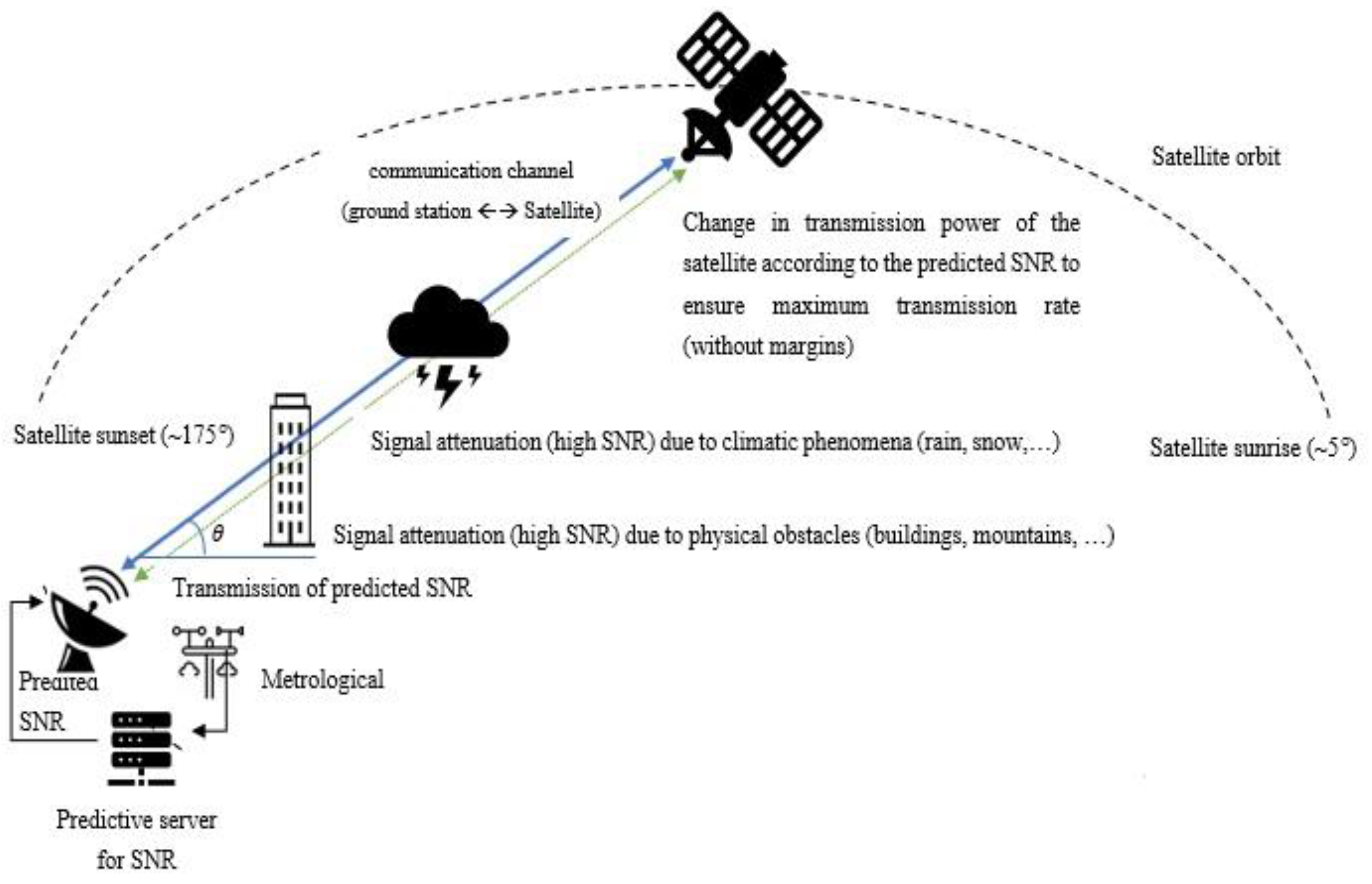
A satellite cruises in a specific orbit while receiving and sending signals to and from a ground station. The ground station is located in a fixed location. Figure 1 depicts the entire satellite communication scene where the ground station, satellite, and orbit are synchronized to enable data transmission between them. The signal route from the satellite to the ground station contains two main sections: from satellite to near ground, designated as A; and from close land to the ground station, designated as B. Section A focuses on predicting the attenuation level of signals from the satellite, passing the free space up to the ground buildings. Section B indicates the remaining signal strength after passing the ground station’s blocking structures. Sections A and B complement each other to predict the initial signal strength by satellite to overcome the accumulated signal attenuation when passing both sections.

Figure 1. The satellite communication scene.

The satellite link budget LB is distributed among the panels, including the P_T transmitter output power (dBm), G_T transmitter antenna gain (dBi), G_R receiver antenna gain (dBi), L_FS free-space propagation loss, and L_M (=L_S + L_R) miscellaneous losses (fading margin, body loss, polarization mismatch, and other losses) (dB). The link budget can be expressed as LB = P_T + G_T + G_R + L_FS + L_M and SNR = $\frac{PT · GT · GR · LFS · LM}{N_0·B}$ where N₀ is the basic noise level, and B is the signal bandwidth. To maintain an SNR that ensures the maximum transmission rate when the signal attenuation changes (L_M decreases or increases), the transmission output power P_T is changed accordingly. Figure 2 depicts the components used for calculating the LB value. We used the STK simulator to obtain synthetic communication data between the satellite and the ground station according to different weather-situation data to prove our approach.

Figure 2. The components used for calculating the LB value.

Typical ground stations in modern urban areas are surrounded by high buildings disturbing the propagation of electromagnetic waves. We focused on the reflections and diffractions signals caused by structures, which lead to reduced signal effectiveness and signal loss.

The combination of predicting the signal attenuation and performing the correction of the transmission intensities make it possible to maintain a proper signal-to-noise ratio (SNR) and prevent transmission interference. For each section, A and B, we developed a separate prediction model using LSTM and an associated Python programming software. We used collected data from the Genesis LEO satellite and corresponding simulated data in the range of 2.4 GHz to 72 GHz. We then executed two LSTM systems, one for each section, to predict the attenuation levels in each part. We reached a less than 2% gap between the predicted and the actual attenuation levels for each piece. We calculated the expected SNR based on this data, the ITU model, and the LSTM neural networks for a second ahead. The signal strength was changed accordingly based on the predicted SNRs, resulting in reduced power consumption. We conducted separate experiments for each frequency. Results show that the predicted measurements for all frequencies were close to the actual value.

In summary, we used LSTM, developed software, good training data, and a testbed with a wide range of frequencies to provide a comprehensive prediction accuracy model. The main novelty of this work is the prediction accuracy, comprehensiveness, and the ability to apply it for more cases.

The rest of this paper is organized as follows: Section 2 outlines related work, Section 3 presents our model for predicting the signal attenuation level due to climate situations and blocking construction near the ground station, Section 4 outlines the experiment setup and the corresponding results for each route section, and in Section 5 we conclude with conclusions and future work. Where applicable, we separated between sections A and B to emphasize the differences.

2. Related Work

Samad et al. [2] provided a comprehensive overview of past and current rain attenuation models, outlining classification, accuracy, and comparison with additional details on the LA rain attenuation (LARA) models. Kalaivaanan et al. [3] suggested antennas with a larger diameter to receive a broader range of data that improves the accuracy of the results and reduces the rain attenuation prediction error. They used a Ka band with an antenna with a diameter of above 7.2 m in tropical regions to prove this. Dahman et al. [4] proposed a binary decision probabilistic method for Ka-frequency rain attenuation forecast using a predetermined threshold. The protocol was adjusted for probabilistic weather forecasts in a communication satellite control loop. Golovachev et al. [5] showed the reduction of the bit error rate for the orthogonal frequency division multiplexing (OFDM) communication link applied for millimeter-waves (MMW, 30 GHz–300 GHz) transmission. Bonev et al. [6] analyzed rain attenuation measurements collected over four years, working at 11, 15, and 19 GHz, and proposed to improve the rain-prediction model’s accuracy coefficients. Bundall et al. [7], focused on the distance factor for MMW links, found that the distance values for the path lengths up to 1 km are inconsistent. They proposed a fix for the distance factor in ITU-R P530.17. Turkmen et al. [8] describe an omnidirectional and circularly polarized antenna for satellite communication applications. It increases the bandwidth of the antenna by 5–6%.

Yeo et al. [9] presented a rain attenuation model for the tropical region with a rainfall rate of 0.01% at the time. It collected input from two satellites operating at Ka-band (WINDS) and Ku-band (GE23), 18.9 GHz and 12.75 GHz, respectively. The gap between the predicted and the actual measures showed that the gap was less than those predicted by the ITU-R, Yamada, DAH, Karasawa, and Ramachandran models. Islam et al. [10] proposed an improvement of ITU-R for tropical regions and 15 GHz frequency. Ahuna et al. [11] offered a combination of rainfall statistics and an ML-based model, which used a neural network trained by rainfall data collected in South Africa for four years. They found that the gap between the predicted and actual results was close, which is better than other models for a short sampling time. Das et al. [12] noticed that a rainfall prediction model applied for tropical regions does not generate the same accuracy when applied to other areas. A proper μ and s model is required to fit other locations, assuming that a large dataset exists for the desired region at different frequencies. Hence, a global model for μ and s is applicable for any area for a time series of rain attenuation. Fadilah and Pratama [13] compared rain attenuation prediction in Indonesia using the ITU-R, Global Crane, and DAH models. The study concluded that ITU-R provides the closest forecast.

Most of the reviewed models relate to the tropical region while ignoring others. Sakir and Atiqul [14] used areas of Bangladesh using 36 GHz to 46 GHz and 46 GHz to 56 GHz bands. They observed that the attenuation varied from 40 dB to 170 dB, which is relatively high. Hence, maintaining the connection for 99.99% of the rainy season required 140 dB and 100 dB, respectively. Ngo, T. et al. [15] explored methods to improve the performance and the accuracy of the SNR prediction for LTE and 5G wireless networks and mobile communications. They achieved less than 1 ms process time and complete accuracy when utilizing time-domain signals for SNR range of (−4, 32) dB and resolution of 2 dB. Kazemi, P. et al. [16] proposed an algorithm for improving the handover decisions between two base stations (BSs), eliminating UE assistance and HO reduction. They used ML to predict the SNR of transmissions between two 5G cellular base stations. Shah et al. [17] proposed an LSTM-based system for predicting multi-directional link quality in mm-wave systems in wireless systems. It simulated multi-cell link and vehicular blockers at 28 GHz and 140 GHz and beamed prediction in an indoor setting at 60 GHz.

Tozer et al. [18] outlined the application and features of high-altitude platforms (HAP) to deliver future broadband wireless communications. The term building entry loss corresponds to the definition made at ITU-R. Ref. [19] defined it as the excess loss due to building walls and other building features. Building entry loss depends on the building type, construction, and electrical parameters of the material used. Measurements of penetration loss of various building materials at 1–8  GHz appear in [20]. The authors of [21] presented electrical parameters of materials of S-band frequencies. Many other aspects influence the building entry loss, such as the receiver’s position inside the building, the transmitter, and so forth, making it difficult to accurately estimate the level of received power inside a building. A decrease of the entry losses into building with floor height can often be observed [22,23]. Entry loss measurements for 2 GHz were reported in [24,25]. Measurements of the spread of the received signal within buildings were reported in [26,27,28]. In Ref. [29], the authors focused on the overall building entry loss and building entry loss as a function of elevation and entry angle and the results of time-delay spread. The authors of Refs. [30,31] presented a new model of the path-loss parameters. Micheli D. et al. [32] described a simple way to measure electric wave attenuation within an indoor scenario, demonstrating attenuation level differences for different wall materials and textures. Al-Hourani et al. [33] proposed a framework for modeling satellite-to-ground signal attenuation in urban environments. They captured the shadowing using measurements collected from a global navigation satellite system (GNSS). The mentioned methods were based on various data analysis methods to identify the contributing parameters to signal loss. This approach requires proof of the truth of the found parameters. Our proposed system is based on accumulated data processed by proven ML methodologies, generating improved and accurate outcomes.

More recent research is found in Lin et al. [34]. In the IoT context, they explored the satellite multicast communication integrated with rate-splitting, multiple-access operating in the same frequency band. The authors of Ref. [35] proposed safe and efficient energy transmission for satellite–ground networks, and Ref. [36] explored power allocation for non-orthogonal, multiple-access satellite–ground networks.

In summary, we reviewed rain attenuation and related prediction models for section A. Some focus on a specific range of frequencies, particular world regions, or wireless systems but do not provide a comprehensive approach covering a broader frequency range or models independent of a specific area. For section B, we reviewed several proposals dependent on particular setups. This work proposes a general prediction model that can be adjusted to comply with any region and a broad spectrum of frequencies.

3. Predicting the Signal Attenuation Level at Free Space (Section A)

3.1. Collecting the SNR and Weather Conditions

We collected data on the SNR and weather conditions in the first stage. Figure 3 depicts an example of the SNR station in December 2019.

Figure 3. SNR measurement collection of the attenuation levels.

3.2. Collecting the Attenuation Levels

In stage 2, we collected the attenuation levels during the satellite transition in orbit for 24 h. They correspond to the angle (θ) changes between the ground station and the satellite position.

3.3. Application of the Prediction Model

In stage 3, we used ITU models to calculate channel damping due to climatic phenomena (clouds, rain, snow, etc.). The ITU-R method uses the concept of a sufficient path length using a reduction factor. The process calculates the long-term statistics of the slant path rain attenuation at a given location for frequencies up to 30 GHz and, provisionally, for higher frequencies. This method involves several steps.

3.3.1. Building the Database for the Learner

We used the collected data related to SNR, climatic conditions, and satellite orbits to comprise a learner database to enable SNR prediction. We used data from three sources: STK simulation linking satellite orbit (time and angle) with channel orientation, weather data from a meteorological database, and SNR data measured by the satellite. Each record in the learner database represents an alignment of these three data sources. The record layout is sampling date and time, angle, temperature, frequency, humidity, bandwidths, and an indication of the passed or lost signal. Table 1 presents examples of the database used for training the deep-learning system.

Table 1. Example of the records used for the training stage. The first and last three records. Reprinted with permission from ref. [1]. Copyright 2021 IEEE.

Index	Time	Azimuth (deg)	Elevation (deg)	Range (km)	EIRP (dEW)	Xmtr Gain (dB)	Xmtr EIRP Intensity	Atmos Loss (dB)	Rain Loss (dB)
1	18:20	79	5	2092	−528.5	−558.5	−539.5	0.3663	0.0024
2	18:21	82	5.048	2088	−528.3	−558.3	−539.3	0.3633	0.0024
3	18:22	86	5.124	2081	−528	−558	−539	0.3587	0.0023
-	-	-	-	-	-	-	-	-	-
589	28:07:00	426	5.136	2081	−527.7	−557	−539	0.3582	0.0023
590	28:08:00	430	5.06	2087	−528	−558	−539.3	0.3629	0.0024
591	28:09:00	433	5	2092	−528.3	−558	−539.5	0.3666	0.0024

3.3.2. Developing the Predictive Models

For the prediction method, we used a deep-learning algorithm that follows the following steps:

• Accept the training and testing dataset—Table 1 is an example of the training and testing dataset required to input the predicting system.
• Execute the prediction deep-learning algorithm—The input and output of the prediction procedure:

$$\begin{array}{l}{X}_{m \times n,d,t}\to Y_{m^{*} \times 1,d,t+\Delta t}\hspace{0.17em}(train\hspace{0.17em}file)\\ X_{\tilde{m} \times n,d^{*},t}\to Y_{{\tilde{m}}^{*} \times 1,d^{*},t+\Delta t}\hspace{0.17em}(Test\hspace{0.17em}file)\end{array}$$

In this section, we denote $X_{m\times n,d,t}$, a dataset of size m with n features collected on day d and at time t. $Y_{m\times 1,d,t}$ is the class labels associated with $X_{m\times n,d,t}$. Therefore, the Δt defines a time variation given a dataset $X_{m\times n,d,t}$ known for d and t.

The following four steps comprise the proposed estimation procedure:

Collect two samples of data, $X_{m\times n,d,t}$ and $X_{m\times n,d,t+\Delta t}$, Δt > 0;

Compute a new training set $Z_{m\times n+1,d}$, using $X_{m\times n,d,t}$ and $Y_{m\times 1,d,t+\Delta t}$ by concatenation, that is $Z_{m\times n+1,d}=[X_{m\times v,d,t};Y_{m\times 1,d,t+\Delta t}]$;

Collect the test set $X_{\tilde{m}\times n,d+\Delta d,t}$ (Δd > 0);

Compute $Y_{\tilde{m}\times 1,d+\Delta d,t+\Delta t}$ using the machine-learning algorithm on $Z_{m\times n+1,d}$ and $X_{\tilde{m}\times n,d+\Delta d,t}$.

3.3.3. Training the Learning System That Predicts the Channel Attenuation

In this stage, we trained the learning system. We used the LSTM model, an artificial neural network designed to recognize patterns in data sequences, such as numerical time series data emanating from neural networks as they have a temporal dimension. We used Matlab libraries to execute the LSTM. Below is the Matlab code:

clc

clear all

close all

session1_DataTrain=xlsread(‘DataTrain_10GHz.csv’,1,’A1:G590′)’;

normalizedData=normalize(session1_DataTrain);

session2=xlsread(‘session2_10GHz.csv’,1,’A1:G585′)’;

normalized_Session2=normalize(session2);

session3=xlsread(‘session3_10GHz.csv’,1,’A1:G506′)’;

normalized_Session3=normalize(session3);

output=xlsread(‘DataTrain_10GHz.csv’,1,’H1:I590′)’;

% import normalized data+sessions+output

numFeatures = 7;

numHiddenUnits1 = 100;

numClasess = 2;

%define the architecture of the neural network

layers = [sequenceInputLayer(numFeatures),lstmLayer(numHiddenUnits1),fullyConnectedLayer(numClasess),regressionLayer];

%define the LSTM network

options = trainingOptions(‘adam’, ...

‘MaxEpochs’, 250, ...

‘GradientThreshold’, 1, ...

‘InitialLearnRate’, 0.005, ...

‘LearnRateSchedule’,’piecewise’, ...

‘LearnRateDropPeriod’, 125, ...

‘LearnRateDropFactor’, 0.2, ...

‘Verbose’, 0, ...

‘Plots’,’training-progress’);

%define the optimizer and learning rate

net=trainNetwork(normalizedData,output,layers,options);

%save the model

outputPrediction_For_Session2=predict(net,normalized_Session2)’;

outputPrediction_For_Session3=predict(net,normalized_Session3)’;

3.3.4. Developing a Model That Ensures the Maximum Transmission Rate

The ground station sends the predicted SNR to the satellite. We used the following model to maintain a constant SNR, which may be different from the expected SNR:

$$\begin{gathered} {\mathrm{SNR}}_{\mathrm{predicted} }-{ \mathrm{SNR}}_{\mathrm{Desired} }=0_{ } \\ \frac{P_T · G_T · G_R · L_{FS} · L_M}{N_0·B}-{\mathrm{SNR}}_{\mathrm{Desired} }=0 \end{gathered}$$

P_T is the transmitter output power, L_M is the miscellaneous losses, L_FS is the free-space path loss, G_T is the transmitting antenna gain, G_R is the receiving antenna gain, N₀ is noise energy, and B is the bandwidths. We achieved the power-saving goal using the two parameters, P_T and L_M. If the signal losses increase, the transmitter needs to increase signal strength and vice versa. This differential power supply saves satellite energy consumption.

3.4. LSTM Neural Network Prediction Experiment across Seasons

For modeling the satellite and its sensors to evaluate performance in real time, we used the Systems Tool Kit^® (STK), used by engineers, mission analysts, and operators. The tool is limited to a 1 s prediction. The experiment setup comprised an LSTM neural network system, a Matlab environment loaded with the code described in Section 3.5, and 98 sample records described in Section 3.5. We built the network using the LSTM method and created a tool that predicts SNR values for a future timeframe. The model succeeded in predicting the SNR sample for the next one second based on the data with a deviation of 1%, which is still reliable. We collected data from satellites, researched and explored optimal ways to build the deep neural network architecture of the LSTM, and chose the parameters which reduced the function loss to a minimum. The LSTM neural network training process receives the 98 training samples and outputs the predicted value for the next timeframe. The method comprises a three-stage process, starting with data collection from the satellite, building, training, and testing the RNN using the LSTM method and then iteratively compiling a prediction of the signal intensity for the next timeframe.

The conceptual LSTM process, starting with all 98 samples, was reduced to 20 and, finally, to the resulting SNR value. We defined a hyper-parameters function and, with many empirical experiments, we found that the optimal parameters converged after four epochs. The parameters are: (a) Loss function: mean absolute error, (b) Optimizer: “Adam”, (c) Activation function: “tanh”, (d) Several epochs to saturation 4, 3 layers: 2 LSTM, 1 dense—First layer: 98 neurons, Second layer: 20 neurons, Last layer: 1 neuron. Figure 4 depicts a chart of a one-month sampling experiment using a 10 GHz frequency. It compares the predicted signal graph generated by the LSTM neural network (left) and the actual signal graph (right). We can see that the two charts are very similar, with an average matching of 93%. We revealed similar results for the next four consecutive months, proving that the prediction accuracy depends on various behaviors across seasons.

Figure 4. Comparison of the actual and predicted signal for one month. Reprinted with permission from ref. [1]. Copyright 2021 IEEE.

3.5. Prediction Experiment for 2.4–72 GHz

We introduced the LSTM-ML process and compared the expected rain and fog attenuation levels to the accurate attenuation results executed over a broad spectrum of signal strengths, from 2.4 GHz to 72 GHz. The experiment began with training the LSTM system using the 913 sample records collected. Figure 5 depicts the results achieved during the ML training process.

Figure 5. The attenuation levels derived from the training data compared to actual data. Reprinted with permission from ref. [1]. Copyright 2021 IEEE.

The top chart presents the trained attenuation levels derived from the training data. The bottom graph depicts the actual attenuation levels collected by the satellite. At this stage, we assumed that the LSTM-ML was appropriately calibrated and ready for the prediction process. We executed the same experiment with the same sampled data but with different signal strengths of 2.4 GHz, 10 GHz, 23 GHz, 48 GHz, and 72 GHz. Figure 6a–e depict the results of the experiments performed for each of the five frequencies. The blue and brick lines represent the actual and predicted attenuation levels. The charts below depict the differences between the two charts. We can see the significant similarity between the two graphs. We can also see that all frames demonstrated similar maps with neglected differences.

Figure 6. (a) Comparison of the predicted data and the actual data for 2.4 GHz; (b) Comparison of the predicted data and the actual data for 10 GHz; (c) Comparison of the predicted data and the actual data for 23 GHz; (d) Comparison of the predicted data and the actual data for 48 GHz; (e) Comparison of the predicted data and the actual data for 72 GHz. Reprinted with permission from ref. [1]. Copyright 2021 IEEE.

4. The Prediction Model When Signal Approaches the Ground Station (Section B)

Several steps predicted the signal attenuation after it passes construction. In this section, we describe in detail the entire process. Following, are the main process steps: measuring the building shadowing loss, setting up the prediction model testbed, constructing the database for the learners, developing the predictive model, training the learning system, and aligning the satellite signal strength.

4.1. Measuring Building Shadowing Loss

Building shadowing loss relates to the transmission loss through a building, as illustrated in Figure 7. Measurements were formulated to calculate values of building shadowing loss to be used in planning frequency sharing between the satellite and ground station. For example, the average loss through a concrete/brick building for a frequency of 11 GHz with vertical and horizontal polarization is 30.1 dB (standard deviation 5.0) for V-Pol and 28.6 dB (standard deviation 5.5) for H-Pol.

Figure 7. Building shadowing loss.

4.2. Setting Up the Prediction Model Testbed

We performed our experiment on a building with a reinforced concrete shear wall structure. Figure 8 depicts the setup of the receiving and sending antennas, and Table 2 is an example of the antenna setup features.

Figure 8. The receiving and the transmitting antennas.

Table 2. The antenna setup features.

Transmitting Antenna	Omni-Directional Vertical Polarization Antenna
Receiving antenna	Horn antenna with vertical polarization
Transmitter	Agilent E8267D signal generator
RF power amplifier	The output power in the test is set to 33 dBm
Receiver	Agilent N9030A signal analyzer

Previous measurements showed high dependency on construction material in determining the primary propagation mode and the amount of attenuation caused by the obstacle. Metal-based construction buildings generated the highest average signal attenuation, 35–40 dB. Concrete caused 25–35 dB and wood 10–25 dB. The transmission was the main propagation mode for wooden and concrete structures. At the same time, it was propagation by diffraction for metal, which increased from the corners towards the center of the building shadow. The attenuation due to diffraction increased from 5.0 dB to 10.0 dB.

To better understand the meaning of the following formulas, Figure 9 describes the context of the elements used in the formulas presented in this section. The free-space loss formula is as follows:

$$L_{fs}=32.45+20·log(d_{\left(m\right)})+20·log(f_{\left(GHz\right)})$$

(1)

where d is the distance defined in Figure 2 and f is the carrier frequency (GHz). Transmitted power is Pt (dBm) and received power is Pr (dBm). The losses through the building are stated as L_E, and sending antenna gain and receiving antenna gain in the transmission path are denoted as G_T and G_R, respectively. Then we obtain Equation (2):

$$P_{t\left(dBm\right)}+\left(G_t-L_{fs}-L_E+G_r\right)=P_{r\left(dBm\right)}$$

(2)

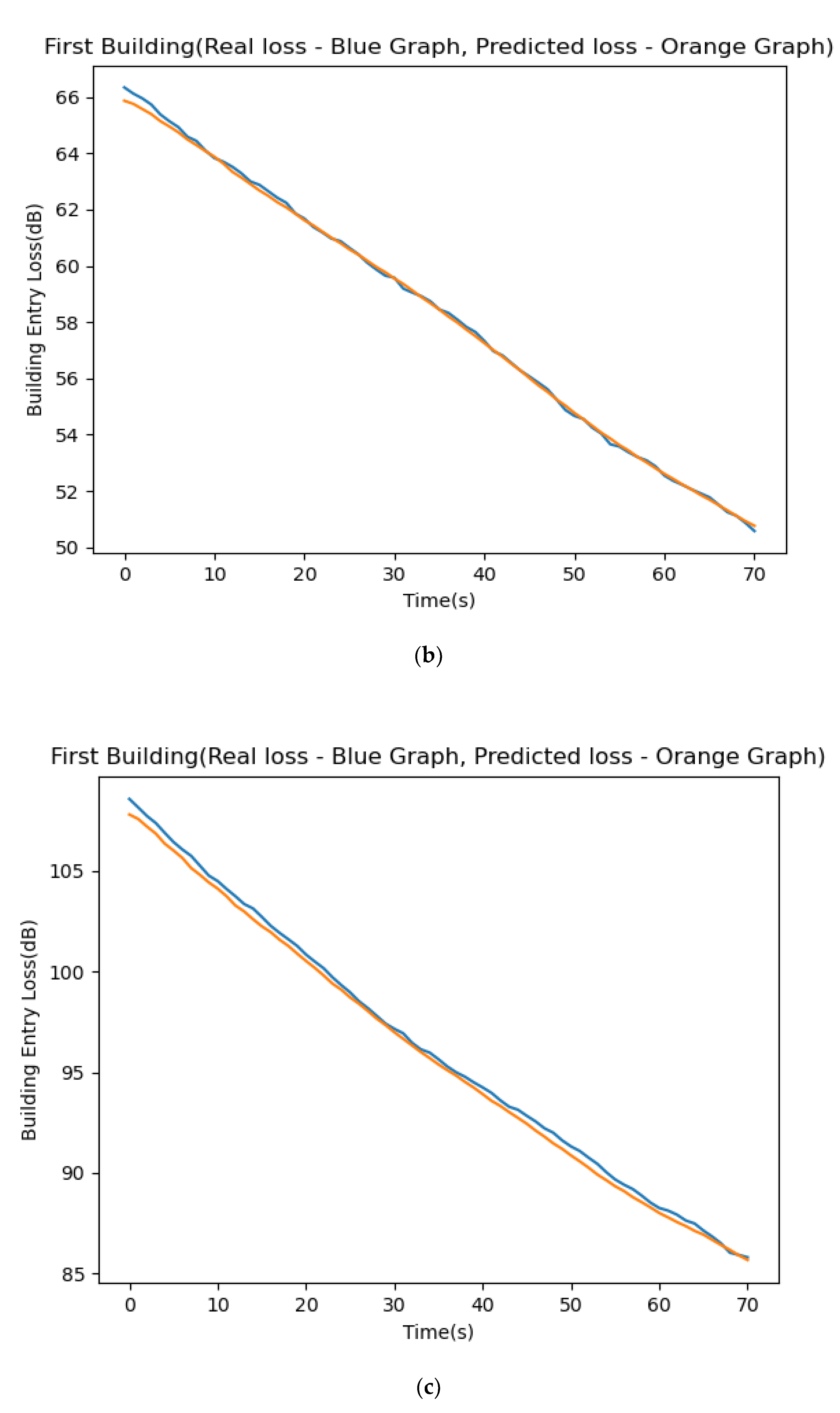
Figure 9. (a) Experiment results for 2.4 GHz; (b): Experiment results for 10 GHz; (c) Experiment results for 23 GHz; (d): Experiment results for 48 GHz; (e) Experiment results for 72 GHz.

Then, the losses through the building are inferred from Equation (3):

$$L_E=\left(P_{t\left(dBm\right)}-P_{r\left(dBm\right)}\right)-L_{fs}+\left(G_t+G_r\right)$$

(3)

The omni-directional antenna used in the experiment is like a half-wave dipole antenna, the gain of which is 2.15 dB, and the normalized directivity function of the electric field of the half-wave dipole antenna is presented by Equation (4):

$$F\left(\theta \right)=sin\left(\theta \right)$$

(4)

From Equation (4), we obtain Equation (5):

$$G_t+G_r=4.3+10·log\left({\left[F\left(\theta \right)\right]}^4\right)=4.3+10·log\left(si{n}^4\theta \right)$$

(5)

The horn antenna is the receiving antenna in the building scenario, so the receiving antenna gain is appropriately considered.

4.3. Constructing the Database for the Learner

In this step, we used the collected data based on (1) the building loss, (2) geometric calculations related to the location of the ground station and the height of the building, and (3) satellite orbits to build a learning database that enabled building loss prediction. The input data came from STK simulation, which links satellite orbit (time and angle) with channel orientation, and geometric calculations relating to a particular scenario. Table 3 depicts an example of the database record layout used for our experiment with a signal frequency of 72 GHz.

Table 3. Dataset records were used for our prediction experiment. Reprinted with permission from ref. [1]. Copyright 2021 IEEE.

Index	Time (min)	Azimuth (deg)	Elevation (deg)	Range (km)	EIRP (dBW)	Xmtr Gain (dB W/Sterad)	Xmtr EIRP Intensity	Atmos Loss (dB)	Urban Terres Loss (dB)
	Date: 24 June 2020 H- 12
1	18:20	79	5	2092	–528.5	–558.5	538.5	0.3663	2.33
2	18:21	82	5.048	2088	–528.3	–558.3	–539.3	0.3633	2.31
3	18:22	86	5.124	2081	–528	–558	–539	0.3587	2.29
-	-	-	-	-	-	-	-	-	-
589	28:07:00	422	5.213	2074	–527.7	–557.7	–538.4	0.3536	2.45
590	28:08:00	426	5.136	2081	–528	–558	–539	0.3582	2.47
591	28:09:00	430	5.06	2087	–528.3	–558.3	–539.3	0.3629	2.5

This dataset will train the deep-learning system described in the next step. Above the table header is the source of each table column.

4.4. Developing the Predictive Model

For the prediction method, a deep-learning (DL) algorithm was used, with the following steps:

(1)

Accept the training and experiment dataset.

As mentioned, Table 2 is an example of the training and experiment dataset required as input for the predicting system. The label class in this case can be binary (e.g., +1 (if attenuation = 0), −1 (if attenuation ≠ 0)).

(2)

Execute the prediction deep-learning algorithm.

The following notation demonstrates the prediction procedure:

$$X_{m\times n,d,t}\to Y_{m^{*}\times 1,d,t+\Delta t} \left(train file\right)$$

(6)

$$X_{\tilde{m}\times n,d^{*},t}\to Y_{{\tilde{m}}^{*}\times 1,d^{*},t+\Delta t} \left(experiment file\right)$$

(7)

X represents samples of satellite data, with matrices size m × n produced at a specific date d and specific time t with class labels m* produced for the same date d but with different time t + Δt. The trained classifier classified the experiment samples (made from latterly date d* and specific time t). Because the algorithm classifier labels for future times, it predicts satellite attenuation.

Satellite data may vary according to days and time (h/min/sec). This section denotes by $X_{m\times n,d,t}$ a dataset of size m with n features, collected on day d and at time (h/min/sec) t and, by $Y_{m\times 1,d,t}$, the class labels associated $X_{m\times n,d,t}$. Therefore, the prediction problem is given a dataset $X_{m\times n,d,t}$ known for every time t to estimate $Y_{\tilde{m}\times 1,d+\Delta d,t+\Delta t}$, where Δd and Δt, respectively, define a variation of day and time (h/min/sec).

The proposed estimation procedure then can be decomposed into four steps:

Collect two samples of data, $X_{m\times n,d,t}$ and $X_{m\times n,d,t+\Delta t}$, Δt > 0;

Compute the class labels $Y_{m\times 1,d,t+\Delta t}$;

Compute a new training set $Z_{m\times n+1,d}$, using $X_{m\times n,d,t}$, and $Y_{m\times 1,d,t+\Delta t}$ by concatenation, that is $Z_{m\times n+1,d}=[X_{m\times v,d,t};Y_{m\times 1,d,t+\Delta t}]$;

Collect the test set $X_{\tilde{m}\times n,d+\Delta d,t}$ (Δd > 0) and compute $Y_{\tilde{m}\times 1,d+\Delta d,t+\Delta t}$ using the machine-learning algorithm on $Z_{m\times n+1,d}$ and $X_{\tilde{m}\times n,d+\Delta d,t}$.

4.5. Training the Learning System

The learning system that predicts the channel attenuation was trained in this stage. Two different methods were used to find a faster and more accurate process. We used the LSTM (long short-term memory) model using Python libraries. LSTM is an artificial neural network designed to recognize patterns in data sequences, such as numerical time series data emanating from sensors, stock markets, and government agencies. RNNs (recurrent neural networks) and LSTMs are different from other neural networks as they have a temporal dimension.

4.6. Aligning the Satellite Signal Strength

The predicted signal-to-noise ratio (SNR) was sent back from the ground station to the satellite. The aim was to maintain a constant level of satellite link budget, which is conveyed by the desired signal-to-noise ratio level and may be different from the predicted signal-to-noise ratio level. We used the following model:

$$SN{R}_{predicted }-SN{R}_{Desired }=0 ➞ \frac{P_T · G_T · G_R · L_{FS}· L_E}{N_0·B}-SN{R}_{Desired }=0$$

(8)

where P_T is transmitter output power, L_E is losses through the building, L_FS is free-space path loss, G_T is the transmitting antenna gain, G_R is the receiver antenna gain, N₀ is noise energy, and B is the bandwidth. Using the two parameters, P_T and L_E, we achieved this goal. If the losses through the building decrease, the transmitter output power needs to increase and vice versa.

4.7. The Setup of the LSTM Experiment

The experiment setup comprised an LSTM L, a Python environment loaded with the code described sample records described in Section 3.5. We built the network using the LSTM method and created a tool that predicts SNR values for a future timeframe. The model succeeded in predicting the SNR sample one second in advance, based on the samples with a loss of 1%, which is still reliable. We collected data from satellites, researched and explored optimal ways to build the deep neural network architecture of LSTM, and chose the parameters which reduced the loss function to a minimum. The LSTM training process loaded the input records to the LSTM neural network. The output was a predicted value for the next timeframe (1 s).

The LSTM mechanism comprises several epochs, starting with the entire input sample, reducing to a smaller number, and reducing to one instance at the final stage. We developed a hyper-parameters function and, with several empirical experiments, we identified the optimal parameters converged after four epochs. The parameters are: (a) Loss function: mean absolute error, (b) Optimizer: “Adam”, (c) Activation function: “tanh”, (d) Number of epochs to saturation: 4, 3 layers: 2 LSTM, 1 dense—First layer: 98 neurons, Second layer: 20 neurons, Last layer: 1 neuron.

We used the LSTM process and compared the predicted building attenuation levels to the actual attenuation results executed over a wide variety of frequencies, from 2.4 GHz up to 72 GHz. The experiment started with training the LSTM system using 913 sample records from the STK satellite simulation connected to its corresponding earth station. Figure 9 depicts the results of the experiments performed for each of the five frequencies. The average difference between the predicted and actual results was below 2%. It can be seen, visually, from the presented figures. The y-axis represents the signal loss through the building in dB. The x-axis represents times (from the moment the ground station discovers the satellite) in seconds or the satellite’s angle (above the ground) in degrees. The blue and orange lines in the top frame represent the actual and predicted attenuation levels, respectively. We can see how close the two charts are and realize that all other figures demonstrate similar charts. We checked the training results, and they resemble the accurate results to a convincing extent. Figure 9a–e depict the comparison of our experiment’s predicted/true signal strength for the frequency range of 2.4–72 GHz.

5. Conclusions and Further Work

This research aimed to predict the degradation of the communication signal transmitted from a satellite until it reaches the ground station. The signal copes at the beginning, with attenuation caused by climate phenomena, and later, when it meets ground constructions surrounding the ground station. We applied LSTM twice to provide two prediction models to cover what the signal is experiencing. This prediction’s impact optimizes the energy consumed by a satellite transmitter to properly propagate microwave signals towards its associated ground station, enabling broadband communication. We proposed a prediction mechanism using LSTM neural networks. We collected and simulated data from the Genesis satellite and built a sampling dataset to serve as the training dataset loaded to the LSTM system. We executed the predicting models for a wide frequencies spectrum and reached excellent predictions. We intend to expand the prediction timeframe (more than one second) further and apply it to other obstacles causing signal attenuation and loss.

References

1. Domb, M.; Leshem, G. Rain Attenuation Prediction for 2.4–72 GHz using LTSM, an artificial recurrent neural network technology. In Proceedings of the 2021 International Conference on Electrical, Communication, and Computer Engineering (ICECCE), Kuala Lumpur, Malaysia, 12–13 June 2021; pp. 1–6. [Google Scholar] [CrossRef]
2. Samad, M.A.; Choi, D.-Y. Learning-Assisted Rain Attenuation Prediction Models. Appl. Sci. 2020, 10, 6017. [Google Scholar] [CrossRef]
3. Kalaivaanan, M.; Sali, A.; Raja Abdullah, R.S.A.; Yaakob, S.; Singh, M.J.; Al-Saegh, A.M. Evaluation of ka-band rain attenuation for satellite communication in tropical regions through a measurement of multiple antenna sizes. IEEE Access 2020, 8, 18007–18018. [Google Scholar] [CrossRef]
4. Dahman, I.; Arbogast, P.; Jeannin, N.; Benammar, B. Rain attenuation prediction model for satellite communications based on the Météo-France ensemble prediction system PEARP. Nat. Hazards Earth Syst. Sci. 2018, 18, 3327–3341. [Google Scholar] [CrossRef]
5. Golovachev, Y.; Pinhasi, G.A.; Pinhasi, Y. Atmospheric Effects on OFDM Wireless Links Operating in the Millimeter Wave Regime. Electronics 2020, 9, 1598. [Google Scholar] [CrossRef]
6. Bonev, B.; Angelov, K.; Altimirski, E. Experimental Estimation and Correction of the Methods for Radio Waves Attenuation Prediction in Rain. ICEST 2012, 2012, 37–38. [Google Scholar]
7. Budalal, A.A.H.; Islam, M.R.; Abdullah, K.; Rahman, T.A. Modification of Distance Factor in Rain Attenuation Prediction for Short-Range Millimeter-Wave Links. IEEE Antennas Wirel. Propag. Lett. 2020, 19, 1027–1031. [Google Scholar] [CrossRef]
8. Ceyhan Turkmen,Mustafa Secmen, Omnidirectional and Circularly Polarized Slotted Antenna Array With Increased Bandwidth Performance by Using Nonidentical Waveguide Slots. AGU-Radio Sci. 2018, 53, 1406–1418. [CrossRef]
9. Yeo, J.X.; Lee, Y.H.; Ong, J.T. Rain Attenuation Prediction Model for Satellite Communications in Tropical Regions. IEEE Trans. Antennas Propag. 2014, 62, 5775–5781. [Google Scholar] [CrossRef]
10. Islam, R.M.; Abdulrahman, Y.A.; Rahman, T.A. An improved ITU-R rain attenuation prediction model over terrestrial microwave links in a tropical region. EURASIP J. Wirel. Commun. Netw. 2012, 2012, 189. [Google Scholar] [CrossRef][Green Version]
11. Ahuna, M.N.; Afullo, T.J.; Alonge, A.A. Rain Attenuation Prediction Using Artificial Neural Network for Dynamic Rain Fade Mitigation. SAIEE Afr. Res. 2019, 110, 11–18. [Google Scholar] [CrossRef]
12. Dalia, D.; Animesh, M. Rain attenuation prediction during rain events in different climatic regions. J. Atmos. Sol.-Terr. Phys. 2015, 128, 1–7. [Google Scholar] [CrossRef]
13. Fadilah, N.; Pratama, R. Comparison of rain attenuation estimation in high frequency in Indonesia region for LAPAN communication satellite. J. Phys. Conf. Ser. 2018, 1130, 012036. [Google Scholar] [CrossRef]
14. Sakir, H.; Atiqul, I. Estimation of Rain Attenuation at EHF bands for Earth-to-Satellite Links in Bangladesh. In Proceedings of the International Conference on Electrical, Computer and Communication Engineering (ECCE), Cox’s Bazar, Bangladesh, 16–18 February 2017. [Google Scholar]
15. Ngo, T.; Kelley, B.T.; Rad, P. Deep Learning Based Prediction of Signal-to-Noise Ratio (SNR) for LTE and 5G Systems. In Proceedings of the 2020 8th International Conference on Wireless Networks and Mobile Communications (WINCOM), Reims, France, 27–29 October 2020. [Google Scholar]
16. Kazemi, P.; Al-Tous, H.; Studer, C.; Tirkkonen, O. SNR Prediction in Cellular Systems based on Channel Charting. In Proceedings of the 2020 IEEE Eighth International Conference on Communications and Networking (ComNet), Hammamet, Tunisia, 27–30 October 2020; pp. 1–8. [Google Scholar] [CrossRef]
17. Shah, S.H.A.; Sharma, M.; Rangan, S. LSTM-Based Multi-Link Prediction for mmWave and Sub-THz Wireless Systems. In Proceedings of the ICC 2020–2020 IEEE International Conference on Communications (ICC), Dublin, Ireland, 7–11 June 2020; pp. 1–6. [Google Scholar] [CrossRef]
18. Tozer, T.C.; Grace, D. High-altitude platforms for wireless communications. Electron. Commun. Eng. J. 2001, 13, 127–137. [Google Scholar] [CrossRef]
19. ITU-R. Propagation Data and Prediction Methods for Planning Short-Range Outdoor Radiocommunication Systems and Radio Local Area Networks in the Frequency Range 300 MHz to 100 GHz. ITU-R P Series, Radiowave Propagation. Recommendation ITURP1411-9. Available online: https://www.itu.int/dms_pubrec/itu-r/rec/p/R-REC-P.1411-9-201706-I!!PDF-E.pdf (accessed on 30 June 2017).
20. Stone, W. Electromagnetic Signal Attenuation in Construction Materials; National Institute of Standards and Technology: Gaithersburg, MD, USA, 1997. [Google Scholar]
21. Baker-Jarvis, J.; Janezic, M.D.; Riddle, B.F.; Johnk, R.T.; Holloway, C.L.; Geyer, R.G.; Grosvenor, C.A. Measuring the Permittivity and Permeability of Lossy Materials: Solids Liquids, Building Material, and Negative Index Materials; National Institute of Standards and Technology: Gaithersburg, MD, USA, 2005. [Google Scholar]
22. Stavrou, S.; Saunders, S.R. Review of constitutive parameters of building materials. In Proceedings of the 12th International Conference on Antennas and Propagation (ICAP 2003), Exeter, UK, 31 March–3 April 2003; pp. 211–215. [Google Scholar]
23. De Toledo, A.F.; Turkmani, A.M.D.; Parsons, J.D. Estimating radio transmission coverage into and within buildings at 900, 1800, and 2300 MHz. IEEE Pers. Commun. 1998, 5, 40–47. [Google Scholar] [CrossRef]
24. Martijn, E.F.T.; Herben, M.H.A.J. Characterization of radio wave propagation into buildings at 1800 MHz. IEEE Antennas Wirel. Propag. Lett. 2003, 2, 122–125. [Google Scholar] [CrossRef]
25. Vogel, W.J.; Torrence, G.W. Propagation measurements for satellite radio reception inside buildings. IEEE Trans. Antennas Propag. 1993, 41, 954–961. [Google Scholar] [CrossRef]
26. Oestges, C.; Paulraj, A.J. Propagation into buildings for broadband wireless access. IEEE Trans. Veh. Technol. 2004, 53, 521–526. [Google Scholar] [CrossRef]
27. Devasirvatham, D.M.J.; Krain, M.J.; Rappaport, D.A.; Banerjee, C. Radio propagation measurements at 850 MHz, 1.7 GHz, and 4 GHz inside two different offices buildings. Electron. Lett. 1990, 26, 445–447. [Google Scholar] [CrossRef]
28. Nobles, P.; Halsall, F. Delay spread measurements within a building at 2 GHz, 5 GHz, and 17 GHz. In Proceedings of the IEE Colloquium on Propagation Aspects of Future Mobile Systems, London, UK, 25 October 1996. [Google Scholar]
29. ITU-Report, P.2346. Compilation of Measurement Data Relating to Building Entry Loss. Available online: https://www.itu.int/pub/R-REP-P.2346 (accessed on 30 December 2021).
30. Perez-Fontan, F.; Hovinen, V.; Schonhuber, M.; Prieto-Cerdeira, R.; Delgado-Penín, J.A.; Teschl, F.; Kyrolainen, J.; Valtr, P. Building entry loss and delay spread measurements on a simulated HAP-to-indoor link at S-band. EURASIP J. Wirel. Commun. Netw. 2008, 2018, 427352. [Google Scholar] [CrossRef]
31. Plets, D.; Joseph, W.; Vanhecke, K.; Tanghe, E.; Martens, L. Simple indoor path loss prediction algorithm and validation in living lab setting. Wirel. Pers. Commun. 2013, 68, 535–552. [Google Scholar] [CrossRef][Green Version]
32. Micheli, D.; Santoni, F.; Delfini, A. Measurement of Electromagnetic Field Attenuation by Building Walls in the Mobile Phone and Satellite Navigation Frequency Bands. IEEE Antennas Wirel. Propag. Lett. 2014, 14, 1. [Google Scholar] [CrossRef]
33. Al-Hourani, A.; Guvenc, I. On Modeling Satellite-to-Ground Path-Loss in Urban Environments. IEEE Commun. Lett. 2021, 25, 696–700. [Google Scholar] [CrossRef]
34. Lin, Z.; Lin, M.; de Cola, T.; Wang, J.-B.; Zhu, W.-P.; Cheng, J. Supporting IoT With Rate-Splitting Multiple Access in Satellite and Aerial-Integrated Networks. IEEE Internet Things J. 2021, 8, 11123–11134. [Google Scholar] [CrossRef]
35. Lin, Z.; Lin, M.; Champagne, B.; Zhu, W.-P.; Al-Dhahir, N. Secure and Energy-Efficient Transmission for RSMA-Based Cognitive Satellite-Terrestrial Networks. IEEE Wirel. Commun. Lett. 2021, 10, 251–255. [Google Scholar] [CrossRef]
36. Lin, Z.; Lin, M.; Wang, J.-B.; de Cola, T.; Wang, J. Joint Beamforming and Power Allocation for Satellite-Terrestrial Integrated Networks With Non-Orthogonal Multiple Access. IEEE J. Sel. Top. Signal. Processing 2019, 13, 657–670. [Google Scholar] [CrossRef]
Publisher’s Note: MDPI stays neutral with regard to jurisdictional claims in published maps and institutional affiliations.
Article Metrics
Citations
Article Access Statistics
Multiple requests from the same IP address are counted as one view.