An Optimal Procedure for the Design of Discrete Constrained Lens Antennas with Minimized Optical Aberrations. Part II: Three-Dimensional Multifocal Architectures

Abstract

Novel three-dimensional discrete lens antennas characterized by a number of focal points ranging from one to five and defined explicitly via analytical equations are presented in the paper. A procedure to derive rotationally symmetric afocal lenses starting from multifocal lenses that are not rotationally symmetric is proposed as well. In addition, an innovative method to identify the focal surface minimizing the optical aberrations is derived. The lenses are compared in terms of optical aberrations and accommodation constraints. The most suitable lens architectures depend mainly on the required angular field of view and magnification factor. It is shown that a reduction by a factor close to 3 in the optical aberrations can be obtained when selecting the most appropriate lens architecture and keeping comparable accommodation constraints. The results, derived exploiting a geometrical optics (GO) formulation, provide useful indications for the preliminary design of constrained lens antennas before adopting full wave rigorous techniques. Three-dimensional discrete lens antennas can offer significant advantages as compared to conventional analog beamforming networks (as those based on Butler matrixes) in terms of frequency bandwidth, number of beams and number of radiating elements.

1. Prior Art

Discrete lens beamforming networks (BFNs) and antennas are also known as bootlace lenses, constrained lenses, or discretized array lenses [1]. Two-dimensional (parallel plate configuration) bootlace lenses have been investigated intensively in the literature starting from some seminal contributions [2,3,4]. The success of the two-dimensional lenses is justified by their design simplicity, their modularity and scalability and several other properties they share with three-dimensional discrete lenses. Two-dimensional constrained lenses can be designed to have more than one focal point. Wide angle scanning capabilities of these lenses in one single plane is well established, being larger for higher number of focal points [1,2,3,4,5].

Three-dimensional lenses have been investigated less. In [5] J.B.L. Rao investigated three-dimensional bootlace lenses having two, three, and four perfect focal points located in a single plane containing the longitudinal axis of the lens. The results of the aperture phase error analysis showed that a lens with a larger number of focal points can be scanned to much larger angles in one plane at the expense of the scanning capability in the orthogonal plane. J.L. McFarland and J.S. Ajioka [6] have proposed a bispherical lens, composed by two portions of spheres with two identical radii, for three-dimensional scanning. J.B.L. Rao [7] generalized this bispherical lens to include two spheres with different radii in order to control the accommodation of the lens. McGrath [8] has introduced a simple three-dimensional lens with flat front and back profiles, homologous elements aligned radially and exhibiting two superimposed foci located in the lens axis. Immediately after, Sole and Smith [9] introduced a three-dimensional lens with flat front profile, back profile with the shape of a saddle, and four focal points. They showed that similar performance in terms of optical aberrations as compared to the McGrath lens can be obtained adopting a more compact lens with curved back profile. C. Rappaport and A. Zaghloul [10] have been also studying three-dimensional lenses having two, three, and four focal points located in a plane containing the longitudinal axis of the lens so only able to perform a two-dimensional type of scanning. C. Rappaport and J. Mason [11] have been considering a five-foci three dimensional discrete lens; however, only a limited numerical investigation has been proposed.

It is important to note that a three-dimensional scanning can be obtained also by cascading two blocks of two-dimensional bootlace lenses as done at Raytheon by Maybell and colleagues [12,13] and by Chan, Rao and Bhattacharyya in [14,15].

In the last 15 years, several developments on three-dimensional constrained lenses have been initiated by the European Space Agency [16,17,18,19,20,21,22]. In [16] in order to improve the transfer of power within the lens and to better control the amplitude tapering and sidelobe level, radiating elements characterized by different apertures have been exploited [18,19,20,21]. In [22] a three-dimensional constrained lens able to operate both in transmission and reception has been proposed for the first time.

The paper is organized as follows. The general properties of three-dimensional discrete lens antennas are presented in Section 2. The relation between degrees of freedom and number of focal points is introduced in Section 3. The magnification property, achievable also with dual reflector antenna systems, is detailed in Section 4. In Section 5, multifocal lenses not rotationally symmetric are compared with afocal lenses rotationally symmetric. A procedure to derive rotationally symmetric afocal lenses starting from multifocal lenses not rotationally symmetric is proposed as well. Twelve different three-dimensional lens architectures, with a number of focal points ranging from one to five, are introduced in Section 6, most of them for the first time. They are presented adopting analytical expressions in a closed form. Only a limited attention has been spent in the literature in the identification of the optimum focal surface which guarantees the minimum optical aberrations. For this reason, in Section 7, an innovative method to identify the focal surface minimizing the optical aberrations is introduced. In Section 8, the five most promising lens architectures are compared in terms of optical aberrations and accommodation constraints.

The most suitable lens architectures depend mainly on the required angular field of view and magnification factor. It is shown that a reduction by a factor close to 3 in the optical aberrations can be obtained when selecting the most appropriate lens architecture and keeping comparable accommodation constraints.

All the results in the paper are derived exploiting a Geometrical Optics (GO) formulation. They provide useful indications for the preliminary design of constrained lens antennas before adopting full wave rigorous techniques. Three-dimensional discrete lens antennas can offer significant advantages as compared to conventional analog beamforming networks (as those based on Butler matrixes) in terms of frequency bandwidth, number of beams and number of radiating elements.

2. General Properties

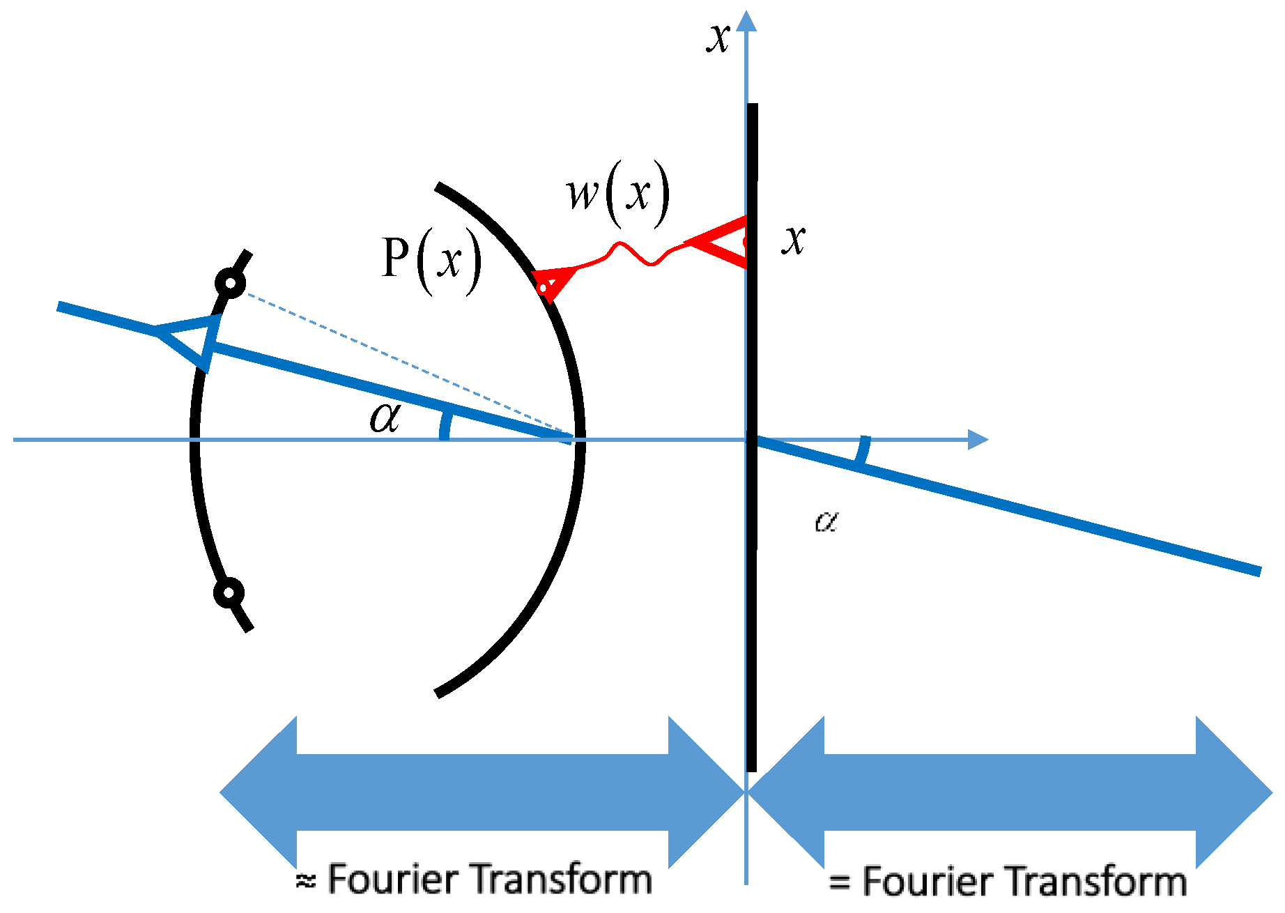
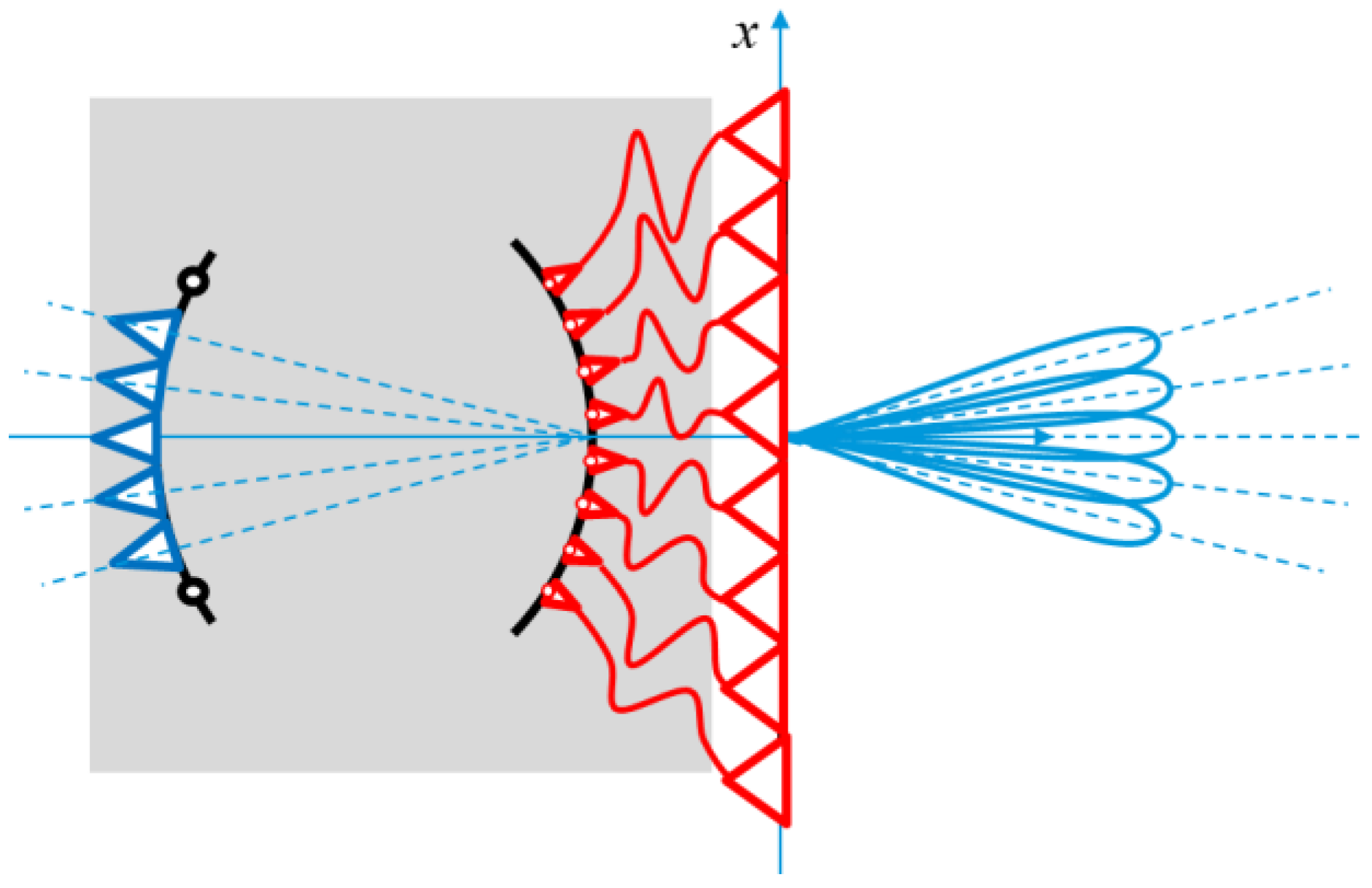
Figure 1 shows the architecture of a discrete lens. They are composed by two parts: a first part, where the fields are propagating in the free-space (for two-dimensional configurations usually an oversized parallel plate waveguide is adopted instead) and a second part, where two arrays of discrete elements are connected with transmission lines (in red in Figure 1). Discrete lenses can be adopted in multibeam antennas systems based on a single feed per beam (SFPB) concept. In fact, by exciting one feed in the focal array, one corresponding beam is generated in the far field.

The relation between the excitations and the far field is approximately equal to a double Fourier transform (Figure 2).

Discrete lenses exhibit some remarkable and unique properties:

a)

almost free-space beamforming;

b)

a true-time delay behavior is guaranteed which is particularly useful in the design of multibeam antennas characterized by large frequency bandwidth;

c)

excellent angular scanning capabilities and limited scan losses because of the onset architecture and multifocal properties;

d)

compatibility with a high number of input and output ports so particularly useful for multibeam antennas characterized by a high number of beams and high number of radiating elements. (i.e., number of beams larger than 1000 can be realized adopting discrete lenses);

e)

complexity that slowly grows with the number of elements and number of beams;

f)

dual polarization functionality (valid for free-space three-dimensional but not for two-dimensional lenses);

g)

possibility, when augmented with active elements, to generate a continuous spot beam coverage adopting only one main aperture instead of the three or four usually adopted in passive single feed per beam (SFPB) antenna configurations based on conventional reflectors or passive lenses.

They are also characterized by some limitations:

1)

high volume and weight with associated difficulty in terms of accommodation;

2)

complexity in implementing a cooling system;

3)

difficulty in feeding the active elements (in the case of active discrete lenses).

The limitation associated to the volume and weight can be mitigated when increasing the operational frequency.

Some additional properties of discrete lenses are:

• Novel types of radiating elements, waveguides (i.e., ridged waveguides, dielectrically filled waveguides, below cut-off radiating elements) can be used in order to increase the bandwidth, obtaining equalized performance in two polarizations, increase the compactness of the solutions, etc.
• As a special condition, the phase shifters can be proportional to the distances between homologous points. This case is important because the lines connecting homologous points, when this condition is valid, can be straight lines.
• The resulting antenna architecture is capable of generating a very high number of beams in fixed spatial directions. The beamforming/antenna architecture can be complemented with a switching network with a number of input ports lower than the overall number of possible beams and a number of output ports equal to the number of input ports of the lens (beams). The switching network can be used to instantaneously activate a reduced number of beams while maintaining the flexibility of a very high number of addressable beams.
• Another feature concerns antennas generating a single beam repointable in a large field of view. In this case the lens-based BFN is simpler as compared to conventional ones even if requires a larger volume.
• Discrete lens BFN and antennas are mainly considered for active antenna systems. However, they may find an applicability also in passive antenna systems. In this case several advantages remain valid (i.e., large scanning domain, large number of beams, large frequency bandwidth, large number of radiating elements.). When considered for a passive antenna system, a significant simplification is obtained (this type of antenna systems does not require the presence of a distributed amplification neither a cooling system). However, in case a multispot beam coverage is required, the typical limitations of passive antenna systems based on the single feed per beam (SFPB) architecture (on the cross-over level and spillover losses) remain present. Considering the significant simplification in terms of cost and complexity, even passive antenna systems based on discrete lenses can find useful applications.
• More than one frequency bandwidth can be exploited in order to mitigate the limitations in terms of accommodation. By adopting in the back of the lens a frequency much larger as compared to the operational frequency (even optical frequencies can be considered) a reduction in size of the back lens can be achieved. The reduction factor is proportional to the ration between the frequency used in the back of the lens as compared to final operational frequency. As an example, for antenna operating at 10 GHz, adopting in the back a frequency of 1 THz a squeezing factor of about 100 could be obtained for the back of the lens and associated optics. This architecture requires of course a frequency conversion with associated cost and limitations.
• Discrete lenses can be complemented with an additional analog or digital beamforming network that acts on the focused beams to offer additional flexibility (e.g., beam shaping, nulling fine steering, etc.) at a lower complexity. This concept is known as beam-space beamforming; the discrete lens acts as a focusing mean to make available the beam-space inputs and the complementing analogue or digital BFN acts in this transformed space. The analog or digital BFN add the needed flexibility but, thanks to the discrete lens focusing, it needs a reduced number of weights per beam.
• If the frequency used in transmission is not too far from the frequency adopted in reception (for instance in the Ku band or in the Q/V band) discrete lens antenna systems can be optimized to work at the same time in transmission and in reception with advantages in terms of accommodations [22].

3. Degrees of Freedom, Number of Foci, Architecture Definition

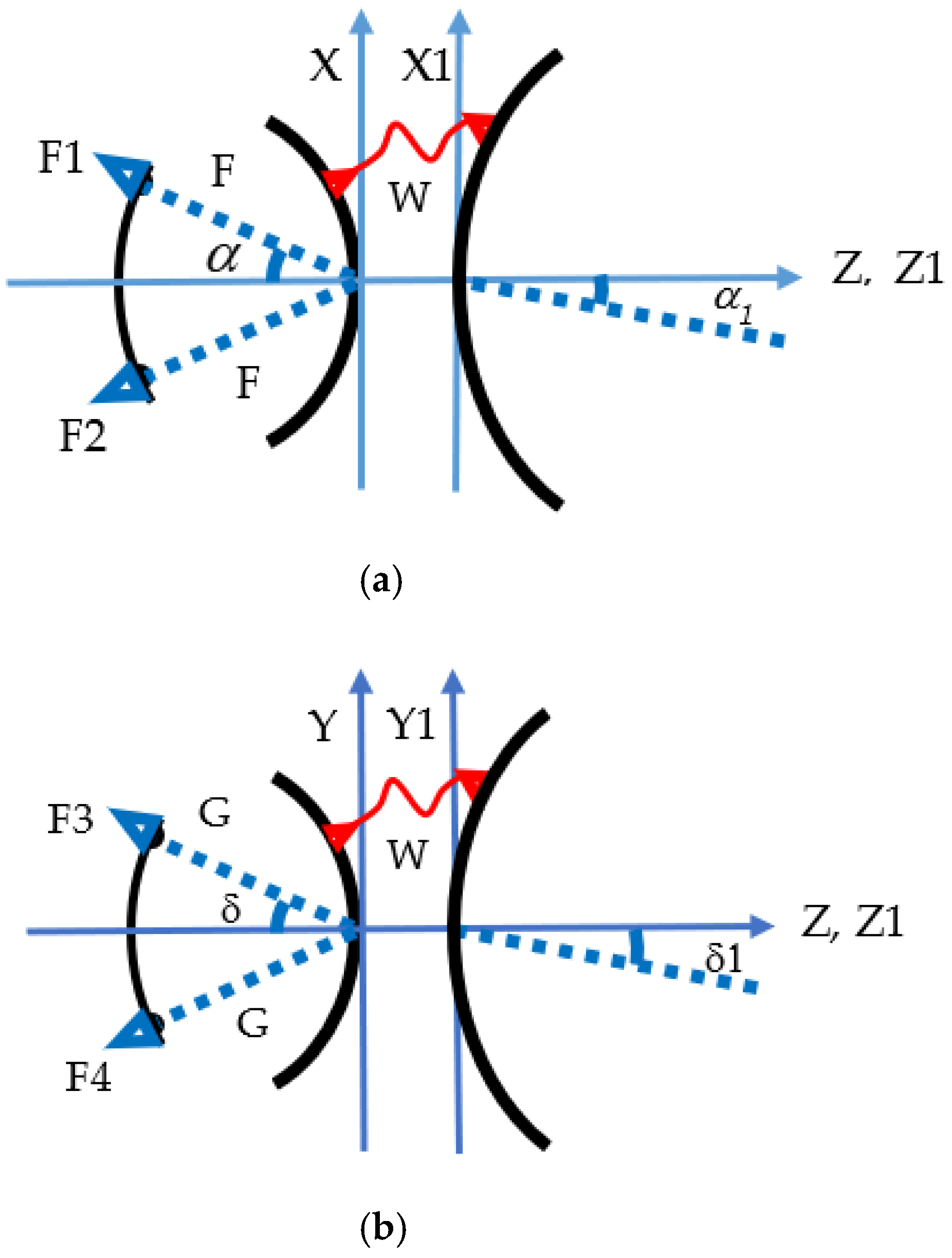
To define a three-dimensional discrete lens, the following seven variables are needed: X, Y, Z (defining the back profile), W (defining the transmission lines length), X1, Y1, Z1 defining the front lens (see Figure 3). Choosing two variables as independent variables (usually the X1 and Y1), 7 − 2 = 5 degrees of freedom remain. In fact, three-dimensional discrete lenses may exhibit up to five foci. Adopting the same reasoning, a two-dimensional lens exhibits 5 − 1 = 4 degrees of freedom so a maximum number of foci equal to four (although an exception exists: the R-2R two-dimensional lens exhibit an infinite number of foci [23,24]). The back of the lens is defined with the Cartesian coordinates (X, Y, Z), the front lens with the Cartesian coordinated (X1, Y1, Z1). The transmission lines lengths with the variable W. The focal points with the letters F1, F2, F3, F4. The focal distance in the X-Z plane with the letter F, the focal distance in the Y-Z plane with the letter G. The angles defining the positions of the foci in the X-Z plane with the letter α in the Y-Z plane with the letter δ. The homologous angles defining the pointing direction of the lens are identified with α1 (in the X-Z plane) and δ1 (in the Y-Z plane). When considering architectures characterized by three foci located in a transversal plane perpendicular to the lens axis and with an angular separation of 120$°$, the common focal length will be denoted by F and the common aperture angle with the letter α.

4. The Magnification or Zooming Capability

In 1967 at Raytheon, it was recognized that an additional degree of freedom is available for two-dimensional bootlace lenses by designing for an off-axis beam to emerge from the array at an angle greater than or less than the angle from the on-axis focus to the driven beam port. This parameter was named the expansion (or compression) factor [12,13]. This magnification factor, that can be considered also a zooming factor, has also been exploited for three-dimensional lenses in [1]. The same property can be obtained with reflector dishes able to magnify the dimensions of a feeding array [25,26].

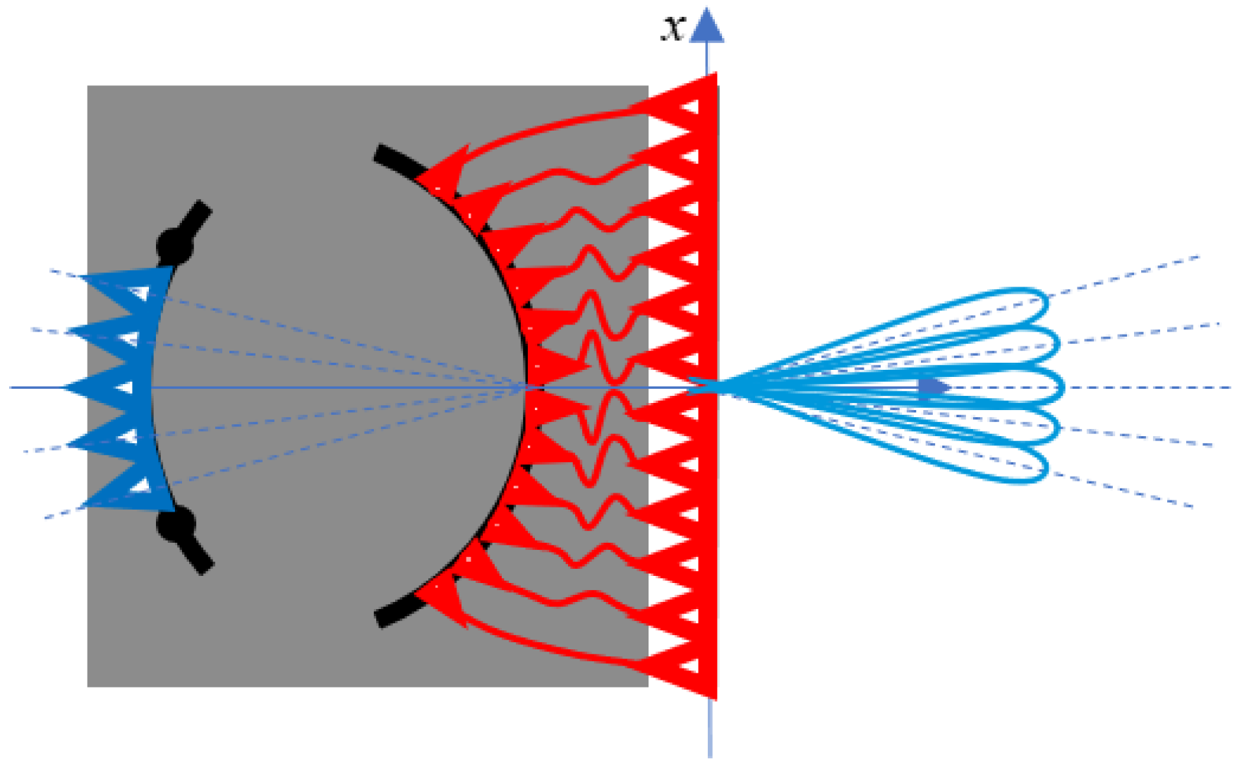
The magnification or zooming capability enables the designer to dimension the back of the discrete lens partially independently from the front aperture with an associated significant flexibility [1]. A first possible architecture which may benefit from this controllable zooming may be a multibeam antenna embarked on a satellite, designed with the back lens aperture smaller as compared to the front one in order to obtain a more compact solution with easier implementation (a reduction of a factor M in linear dimensions imply a reduction of a factor M³ in terms of volume!), see Figure 4.

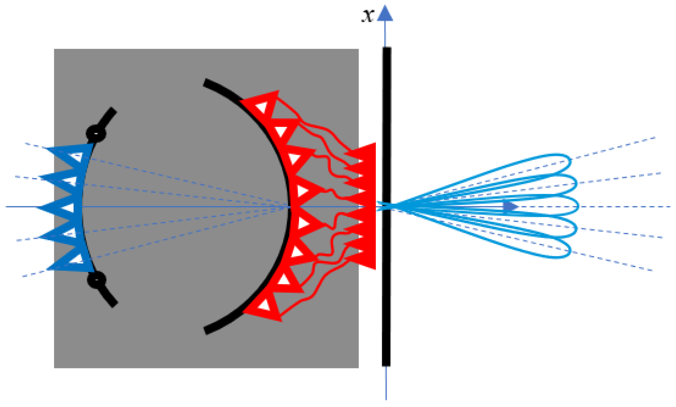
A second architecture exploiting the opposite type of zooming can be an antenna based on discrete lenses designed with the back larger as compared to the front in order to obtain an enlarged field of view with a reduced scanning on the back of the lens (see Figure 5). The penalty associated to the larger dimensions of the back lens can be acceptable for a ground professional or gateway antenna considering the magnified field of view associated to this solution. This second type of zooming can be useful also for BFN and antennas to be installed onboard a satellite. As an example, on-board satellites flying on medium or low Earth orbits (MEO or LEO), active antennas start to replace several passive antennas based on reflectors. As a consequence, the aperture available for installing the antenna can be significantly larger as compared to the minimum physical antenna aperture so allowing the installation of a lens antenna with a back aperture larger as compared to the radiating aperture with the advantage of an enlarged field of view because of the zooming property.

In the paper the magnification or zooming factor is indicated with letter M and can be defined:

$$\begin{array}{c}\sin (\mathsf{\alpha }1)=\sin (\mathsf{\alpha })\mathrm{M},\cos (\mathsf{\alpha }1)={(1-{(\sin (\mathsf{\alpha })\mathrm{M})}^2)}^{\frac{1}{2}}\\ \sin (\mathsf{\delta }1)=\sin (\mathsf{\delta })\mathrm{M},\cos (\mathsf{\delta }1)={(1-{(\sin (\mathsf{\delta })\mathrm{M})}^2)}^{\frac{1}{2}}\end{array}$$

In addition, in order to simplify the analytical equations, the following abbreviations are used:

$$\begin{array}{c}\mathrm{sa}=\sin (\mathsf{\alpha }),\mathrm{ca}=\cos (\mathsf{\alpha }),\\ \mathrm{sd}=\sin (\mathsf{\delta }),\mathrm{cd}=\cos (\mathsf{\delta }),\\ \mathrm{sa}1=\sin (\mathsf{\alpha }1),\mathrm{ca}1=\cos (\mathsf{\alpha }1),\\ \mathrm{sd}1=\sin (\mathsf{\delta }1),\mathrm{cd}1=\cos (\mathsf{\delta }1),\end{array}$$

5. Multifocal Lenses Not Rotationally Symmetric vs. Afocal Lenses Rotationally Symmetric

In the paper discrete lenses characterized by a number of foci ranging from one to five are considered. The case of afocal lenses which do not exhibit any perfect focal point, is considered as well. As usual, a focal point is defined according to the geometrical optics (GO) law and satisfies the following equi-length path condition: when a spherical wave is originated by one focal point and illuminates the back lens via the free-space, all the signals received by the back elements of the lens are properly delayed with the transmission lines and reach the homologous elements in the front lens. Adding to the corresponding phase paths the distances between the elements of the front lens to an assigned plane (perpendicular to the desired plane wave pointing direction) an equi-length path condition should be valid. Accordingly for every focal point an equi-length path equation is enforced. The system of equations to be solved (with a number of equations equal to the number of focal points) contains the unknowns in linear and quadratic forms. This system is ill-condition so small modifications in a single unknown or parameter can bring strong changes in all the other ones. For this reason, numerical optimization procedures can be completely ineffective in the design of discrete lens antennas. In addition, partial or global convergence is requiring intensive calculations. For small angles, i.e., for a limited angular field of view, all the solutions tend to be quite similar and accurate, so it is better to compare different solutions for large field of view (i.e., for scanning directions equal or larger than 45°). In these conditions, different lens antennas behave in a completely different way and some solutions are clearly better in terms of optical aberrations, in terms of compactness, or in terms of orientation of the back lens aperture versus the focal array curve. The last condition in fundamental in order to guarantee a good power transfer inside the lens so to minimize the power reflected by the back part of the lens or not intercepted by the lens itself. As a general rule, by increasing the focal distance versus the lens apertures the optical aberrations decrease. However, different solutions with comparable focal distance may behave quite differently. So a natural design objective consists in minimizing the optical aberrations for an assigned maximum focal distance so for an assigned maximum volumetric envelope of the lens antenna.

Except for the constrained lens characterized by one single focus, most of the configurations presented in the next section are not rotationally symmetric. This means that they do not have all rotationally symmetric variables (i.e., front profile, back profile, W, azimuthal angle defining the back elements vs azimuthal angle defining the front elements) but they may have some of them that are rotationally symmetric. Usually, the multifocal bootlace lenses present an angular symmetry by 120° or 180° depending on the disposition of the foci. When considering the optical aberrations, their maximum value are usually associated to (a) the maximum scanning angles, (b) to the points of the lens located on the external rim, and (c) to azimuthal angles intermediate between the angles associated to planes containing the perfect foci. If for instance, three foci are located in the azimuthal planes characterized by ϕ = 0°, 120° and 240°, the maximum aberrations are present in the planes characterized by ϕ = 60°, 180° and 300°. If, instead, four foci are located in the azimuthal planes characterized by ϕ = 0°, 90°, 180° and 270°, the maximum aberrations are present in the planes characterized by ϕ = 45°, 135°, 225° and 315°.

Starting from a not rotationally symmetric lens, obtaining a rotationally symmetric one may offer important advantages. First of all, the lens manufacturability and cost result being significantly improved. This consideration applies not only for the profiles but also for the connections (i.e., coaxial cables or waveguides) between homologous elements. A second good reason to make a rotationally symmetric lens is related to the optical aberrations. In facts, instead of having a minimum aberration value in three or four planes and a maximum one in the intermediate planes, is better to have a unique intermediate value for the aberrations in all the planes. Finally, also the optimized focal arc results being rotationally symmetric and the performance result being identical in all azimuthal angles. Related to this point, a fourth important one should be mentioned: if all the variables are rotationally symmetric the optimization could be limited to a single plane with significant benefits in terms of calculation times. These homogenized symmetric lenses exhibit, instead of a discrete number of foci, a ring of pseudo-foci. In case a central axial focus is present, the homogenization tends to maintain this axial focus unchanged.

A simple way to obtain a symmetric lens is the following. One starts defining some points in the front aperture whose transversal coordinates (X1 and Y1) are located in a circle. These points are characterized by the same radial coordinate ρ1. For every point, the profile of the front lens element Z1, the phase shifter W, and the coordinates of the homologous element in the back lens (X and Y) are derived analytically. The average value for Z, Z1 and W can be obtained simply making an average between a sufficient number of values. Evaluating this average analytically in a closed form is not usually possible. Regarding the average value to be used for the transversal coordinates, two solutions have been tested. The first consists in evaluating for every ρ1 associated to the generic point in the front lens, the ρ value associated to the homologous back element. Then, an average between several ρ values permits finding an average ρ. A second preferred solution consists in deriving analytically the generic ρ value, considering the square of this quantity, and then evaluating the average ρ squared value. From this average value, considering the square root, an estimation of the average ρ value is derived. This second solution is preferred because, in some cases, as it will be clear in the next section, the average value ρ squared can be obtained analytically while usually the average ρ value cannot be obtained analytically. It has been verified that the differences between the two average ρ values are limited (usually 5–10% of difference).

A final important remark has to be made: when deriving a rotationally symmetric lens starting from a non-rotationally symmetric one, the maximum aberrations result always improved and, of course, are rotationally symmetric as well. In practice the curve representing the maximum aberrations versus the scanning angle (evaluated as compared to the lens axis) is always comprised between the best and the worst curve relevant to the non-rotationally symmetric one. Two-dimensional non focal or afocal lenses have been considered in [27].

6. Derivation and Definition of Multifocal Lenses

All the analytical solutions proposed in the paper were derived using the symbolic calculation software Mupad available in Matlab. All the equations were intensively validated. The multifocal property was verified, and the variables assume only real and not complex values. Often multiple solutions were derived (up to 16 different solutions in the case of some lenses exhibiting four focal points) and the acceptable ones were selected. In the following, the most significant multifocal three-dimensional lens architectures are reported.

6.1. Spherical-Planar Lens with a Single Focal Point

The front is flat, the back is spherical (with radius H), the unique focal point is located in the center of the sphere, the phase shifts are identical. The perfect focalization is guaranteed only in the direction of the lens axis. This lens is not new but it is reported here because it represents an important reference and it is particularly simple to define and manufacture.

$$\mathrm{Z}=-\mathrm{H}+\mathrm{sqrt}({\mathrm{H}}^2-{\mathrm{X}}^2-{\mathrm{Y}}^2);$$

$$\mathrm{Z}1=0;\mathrm{W}=0;$$

The positions of the elements of the back lens as compared to the homologous elements in the front lens are undetermined. This means that any choice guarantees the perfect focalization of the signals along the axis when the source is located in the focal point. However, the relation between back and front element positions has an impact on the scanning performance of the lens. It is usually selected a proportionality between the coordinates of homologous elements:

$$\begin{array}{c}\mathrm{X}=\mathrm{X}1\mathrm{M}=\mathsf{\rho }1\mathrm{M}\cos (\mathsf{\varphi });\\ \mathrm{Y}=\mathrm{Y}1\mathrm{M}=\mathsf{\rho }1\mathrm{M}\sin (\mathsf{\varphi });\end{array}$$

Clearly, the spherical-planar lens does not represent the only single focus constrained lens. One could consider also a lens with a flat front profile, and arbitrary back profile, and homologous elements radially aligned and with positions satisfying the equi-path propagation length. The shape of the back profile can be selected in order to guarantee a good amplitude matching in the back lens and to modify the position of the focal arc. As a rule of thumb, as for the two-dimensional lenses, when the back profile flattens, the optimal focal arc curves more. The phase shifters W represent the only unknown in the design and are derived enforcing a single axial focal point.

6.2. Discrete Lens with Flat Front and Back Profiles and Three Foci

Both the front and back profiles are assumed to be flat (i.e., Z = Z1 = 0). The three residual degrees of freedom are used to enforce three focal points located in the same plane perpendicular to the lens axis and with equiangular distance (120°). Two different solutions have been derived: one with the coordinates of the front lens as independent variables, one with the coordinates of the back lens as independent variables. Both solutions include an arbitrary zooming factor M. In the first solution the transversal coordinates of the front lens (X1, Y1) are selected as independent variables, as is usually done. In the second solution the transversal coordinates of the back lens (X, Y) are selected as independent variables. Assuming that the three unknowns are the transversal coordinates of the back lens (X and Y) and the phase shift (W), these are the equations defining the lens:

$$\begin{array}{l}\mathrm{X}=\frac{\mathrm{F}\mathrm{M}\left(\mathrm{X}{1}^2\mathrm{Msa}-\mathrm{Y}{1}^2\mathrm{Msa}\right)}{4\left(\mathrm{X}{1}^2{\mathrm{M}}^2+\mathrm{Y}{1}^2{\mathrm{M}}^2-{\mathrm{f}}^2\right)}\\ -(\mathrm{M}(2\mathrm{X}1(-2.25\mathrm{X}{1}^4\mathrm{Y}{1}^2{\mathrm{M}}^6{\mathrm{sa}}^2+2.25\mathrm{X}{1}^4{\mathrm{F}}^2{\mathrm{M}}^4{\mathrm{sa}}^2+1.5\mathrm{X}{1}^2\mathrm{Y}{1}^4{\mathrm{M}}^6{\mathrm{sa}}^2\\ +4.5\mathrm{X}{1}^2\mathrm{Y}{1}^2{\mathrm{F}}^2{\mathrm{M}}^4{\mathrm{sa}}^2-2\mathrm{X}{1}^2{\mathrm{F}}^4{\mathrm{M}}^2{\mathrm{sa}}^2-4\mathrm{X}{1}^2{\mathrm{F}}^4{\mathrm{M}}^2-0.25\mathrm{Y}{1}^6{\mathrm{M}}^6{\mathrm{sa}}^2\\ +2.25\mathrm{Y}{1}^4{\mathrm{F}}^2{\mathrm{M}}^4{\mathrm{sa}}^2-2\mathrm{Y}{1}^2{\mathrm{F}}^4{\mathrm{M}}^2{\mathrm{sa}}^2-4\mathrm{Y}{1}^2{\mathrm{F}}^4{\mathrm{M}}^2+4{\mathrm{F}}^6){}^{\frac{1}{2}}-\mathrm{Y}{1}^4{\mathrm{M}}^3\mathrm{sa}\\ +3\mathrm{X}{1}^2\mathrm{Y}{1}^2{\mathrm{M}}^3\mathrm{sa}))/\left(4\mathrm{F}\left(\mathrm{X}{1}^2{\mathrm{M}}^2+\mathrm{Y}{1}^2{\mathrm{M}}^2-{\mathrm{F}}^2\right)\right)\end{array}$$

$$\begin{array}{l}\mathrm{Y}=\left(0.75\mathrm{X}1\mathrm{Y}1{\mathrm{M}}^2\mathrm{sa}\right)/\mathrm{F}-(\mathrm{X}1\left(0.25\mathrm{Y}1\mathrm{M}\left(\mathrm{saY}{1}^2{\mathrm{M}}^3+2{\mathrm{saF}}^2\mathrm{M}\right)-0.75\mathrm{Y}1{\mathrm{M}}^2\mathrm{sa}\left({\mathrm{F}}^2-\mathrm{Y}{1}^2{\mathrm{M}}^2\right)\right)\\ +0.5\mathrm{Y}1\mathrm{M}(-2.25\mathrm{X}{1}^4\mathrm{Y}{1}^2{\mathrm{M}}^6{\mathrm{sa}}^2+2.25\mathrm{X}{1}^4{\mathrm{F}}^2{\mathrm{M}}^4{\mathrm{sa}}^2+1.5\mathrm{X}{1}^2\mathrm{Y}{1}^4{\mathrm{M}}^6{\mathrm{sa}}^2\\ +4.5\mathrm{X}{1}^2\mathrm{Y}{1}^2{\mathrm{F}}^2{\mathrm{M}}^4{\mathrm{sa}}^2-2\mathrm{X}{1}^2{\mathrm{F}}^4{\mathrm{M}}^2{\mathrm{sa}}^2-4\mathrm{X}{1}^2{\mathrm{F}}^4{\mathrm{M}}^2-0.25\mathrm{Y}{1}^6{\mathrm{M}}^6{\mathrm{sa}}^2\\ +2.25\mathrm{Y}{1}^4{\mathrm{F}}^2{\mathrm{M}}^4{\mathrm{sa}}^2-2\mathrm{Y}{1}^2{\mathrm{F}}^4{\mathrm{M}}^2{\mathrm{sa}}^2-4\mathrm{Y}{1}^2{\mathrm{F}}^4{\mathrm{M}}^2+4{\mathrm{F}}^6){}^{\frac{1}{2}})/(\mathrm{F}(\mathrm{X}{1}^2{\mathrm{M}}^2\\ +\mathrm{Y}{1}^2{\mathrm{M}}^2-{\mathrm{F}}^2)\end{array}$$

$$\begin{array}{l}\mathrm{W}=\mathrm{F}+\left(0.5\right(-2.25\mathrm{X}{1}^4\mathrm{Y}{1}^2{\mathrm{M}}^6{\mathrm{sa}}^2+2.25\mathrm{X}{1}^4{\mathrm{F}}^2{\mathrm{M}}^4{\mathrm{sa}}^2+1.5\mathrm{X}{1}^2\mathrm{Y}{1}^4{\mathrm{M}}^6{\mathrm{sa}}^2\\ +4.5\mathrm{X}{1}^2\mathrm{Y}{1}^2{\mathrm{F}}^2{\mathrm{M}}^4{\mathrm{sa}}^2-2\mathrm{X}{1}^2{\mathrm{F}}^4{\mathrm{M}}^2{\mathrm{sa}}^2-4\mathrm{X}{1}^2{\mathrm{F}}^4{\mathrm{M}}^2-0.25\mathrm{Y}{1}^6{\mathrm{M}}^6{\mathrm{sa}}^2\\ +2.25\mathrm{Y}{1}^4{\mathrm{F}}^2{\mathrm{M}}^4{\mathrm{sa}}^2-2\mathrm{Y}{1}^2{\mathrm{F}}^4{\mathrm{M}}^2{\mathrm{sa}}^2-4\mathrm{Y}{1}^2{\mathrm{F}}^4{\mathrm{M}}^2+4{\mathrm{F}}^6){}^{\frac{1}{2}})-(\mathrm{X}{1}^3{\mathrm{M}}^3{\mathrm{sa}}^2)/4\\ +0.75\mathrm{X}1\mathrm{Y}{1}^2{\mathrm{M}}^3\mathrm{sa})/(\mathrm{X}{1}^2{\mathrm{M}}^2+\mathrm{Y}{1}^2{\mathrm{M}}^2-{\mathrm{F}}^2)\end{array}$$

If, vice versa, one assumes that the three unknowns are the transversal coordinates of the front lens (X1 and Y1) and the phase shift (W), these are the equations that completely define the lens:

$$\begin{array}{c}\mathrm{X}1=(1/3{({\mathrm{X}}^2+\mathrm{saXF}+{\mathrm{Y}}^2-\sqrt{3}\mathrm{saYF}+{\mathrm{F}}^2)}^{\frac{1}{2}}-2/3{({\mathrm{X}}^2-2\mathrm{saXF}+{\mathrm{Y}}^2+{\mathrm{F}}^2)}^{\frac{1}{2}}\\ +1/3{({\mathrm{X}}^2+\mathrm{saXF}+{\mathrm{Y}}^2+\sqrt{3}\mathrm{saYF}+{\mathrm{F}}^2)}^{\frac{1}{2}})/(\mathrm{Msa})\end{array}$$

$$\begin{array}{l}\mathrm{Y}1=(\sqrt{3}/3{({\mathrm{X}}^2+\mathrm{saXF}+{\mathrm{Y}}^2+\sqrt{3}\mathrm{saYF}+{\mathrm{F}}^2)}^{\frac{1}{2}})/(\mathrm{Msa})\\ -(\sqrt{3}/3{({\mathrm{X}}^2+\mathrm{saXF}+{\mathrm{Y}}^2-\sqrt{3}\mathrm{saYF}+{\mathrm{F}}^2)}^{\frac{1}{2}})/(\mathrm{Msa})\end{array}$$

$$\begin{array}{c}\mathrm{W}=\mathrm{F}-1/3{({\mathrm{X}}^2-2\mathrm{saXF}+{\mathrm{Y}}^2+{\mathrm{F}}^2)}^{\frac{1}{2}}-1/3{({\mathrm{X}}^2+\mathrm{saXF}+{\mathrm{Y}}^2-\sqrt{3}\mathrm{saYF}+{\mathrm{F}}^2)}^{\frac{1}{2}}\\ -1/3{({\mathrm{X}}^2+\mathrm{saXF}+{\mathrm{Y}}^2+\sqrt{3}\mathrm{saYF}+{\mathrm{F}}^2)}^{\frac{1}{2}}\end{array}$$

It is interesting to note that usually discrete lens BFN are solved assuming the transversal coordinated of the front lens as independent variables (i.e., X1 and Y1). For this specific lens, the three equations associated to the three focal points may be solved also as a function of the back transversal coordinates (i.e., X and Y). Z = Z1 = 0. The back lens proves to be larger compared to the front one. It seems to be impossible to derive analytically the average squared radius for the back lens.

$${\mathsf{\rho }}_{\mathrm{squared}}=\frac{{{\displaystyle \int }}_0^{2\mathsf{\pi }}({\mathrm{X}}^2+{\mathrm{Y}}^2)\mathrm{d}\mathsf{\varphi }}{2\mathsf{\pi }}$$

However, the numerical average of the previous quantities can be easily evaluated.

6.3. The Discrete Lens Derived by McGrath with Flat Front and Back Profiles and Two Coinciding Foci

Keeping Z = Z1 = 0, i.e., maintaining the front and back profiles flat, and using a third degree of freedom to ensure that homologous elements are located in the same radial direction (i.e., they are characterized by the same azimuthal angle) the McGrath lens [8] is obtained. The residual two degrees of freedom correspond to two focal points that in this lens are collocated in a point of the lens longitudinal axis. For the McGrath lens the phase shifters are given by:

$$\mathrm{W}=\mathrm{F}-{({\mathrm{X}}^2+{\mathrm{Y}}^2+{\mathrm{F}}^2)}^{\frac{1}{2}}$$

where F is the axial focal distance defining the positions of the two collocated foci on the axis. In this lens the radial coordinate of the back elements versus the radial coordinate of the homologous elements in the front lens is not determined. To derive the radial coordinates of the back lens the considerations done for the previous lens can be reused.

6.4. The Discrete Lens Derived by Sole and Smith with Four Foci

The lens is a three-dimensional discrete lens with four coplanar perfect foci in a plane perpendicular to the lens axis. Three foci exhibit an equiangular distance (120$°$) and one is placed in the centre exactly on the lens axis. The front lens is forced to be flat (Z1 = 0). This configuration was proposed by Sole and Smith in [9]. Here the solutions in explicit analytical form are presented for the first time. The back lens profile is not rotationally symmetric but looks like a saddle.

$$\begin{array}{c}\mathrm{X}=\mathrm{X}1\mathrm{M}-(0.5\mathrm{X}{1}^3{\mathrm{M}}^3\cos {(0.5\mathsf{\alpha })}^2)/{\mathrm{F}}^2-(0.25\mathrm{X}{1}^2{\mathrm{M}}^2\mathrm{sa})/\mathrm{F}+(0.25\mathrm{Y}{1}^2{\mathrm{M}}^2\mathrm{sa})/\mathrm{F}\\ -(0.5\mathrm{X}1\mathrm{Y}{1}^2{\mathrm{M}}^3\cos {(0.5\mathsf{\alpha })}^2)/{\mathrm{F}}^2\end{array}$$

$$\begin{array}{c}\mathrm{Y}=\mathrm{Y}1\mathrm{M}-(0.5\mathrm{Y}{1}^3{\mathrm{M}}^3)\cos {(0.5\mathsf{\alpha })}^2)/{\mathrm{F}}^2+(0.5\mathrm{X}1\mathrm{Y}1{\mathrm{M}}^2\mathrm{sa})/\mathrm{F}\\ -(0.5\mathrm{X}{1}^2\mathrm{Y}1{\mathrm{M}}^3\cos {(0.5\mathsf{\alpha })}^2)/{\mathrm{F}}^2\end{array}$$

$$\mathrm{W}=(\mathrm{X}{1}^2{(\mathrm{saM})}^2+\mathrm{Y}{1}^2{(\mathrm{saM})}^2)/(4\mathrm{F}-4\mathrm{Fca})$$

$$\begin{array}{l}\mathrm{Z}=-\mathrm{Fca}-(-0.25\mathrm{X}{1}^6{\mathrm{M}}^6{\mathrm{sa}}^6-\mathrm{X}{1}^5{\mathrm{FM}}^5\sin {\left(0.5\mathsf{\alpha }\right)}^2{\mathrm{sa}}^5-0.75\mathrm{X}{1}^4\mathrm{Y}{1}^2{\mathrm{M}}^6{\mathrm{sa}}^6\\ +3\mathrm{X}{1}^4{\mathrm{F}}^2{\mathrm{M}}^4\sin {\left(0.5\mathsf{\alpha }\right)}^2{\mathrm{sa}}^4+0.5\mathrm{X}{1}^4{\mathrm{F}}^2{\mathrm{M}}^4{\mathrm{sa}}^6+2\mathrm{X}{1}^3\mathrm{Y}{1}^2{\mathrm{FM}}^5\sin {\left(0.5\mathsf{\alpha }\right)}^2{\mathrm{sa}}^5\\ +8\mathrm{X}{1}^3{\mathrm{F}}^3{\mathrm{M}}^3\sin {\left(0.5\mathsf{\alpha }\right)}^2{\mathrm{sa}}^3-2\mathrm{X}{1}^3{\mathrm{F}}^3{\mathrm{M}}^3{\mathrm{sa}}^5-0.75\mathrm{X}{1}^2\mathrm{Y}{1}^4{\mathrm{M}}^6{\mathrm{sa}}^6\\ +6\mathrm{X}{1}^2\mathrm{Y}{1}^2{\mathrm{F}}^2{\mathrm{M}}^4\sin {\left(0.5\mathsf{\alpha }\right)}^2{\mathrm{sa}}^4+\mathrm{X}{1}^2\mathrm{Y}{1}^2{\mathrm{F}}^2{\mathrm{M}}^4{\mathrm{sa}}^6\\ +4\mathrm{X}{1}^2{\mathrm{F}}^4{\mathrm{M}}^2\sin {\left(0.5\mathsf{\alpha }\right)}^2{\mathrm{sa}}^4-16\mathrm{X}{1}^2{\mathrm{F}}^4{\mathrm{M}}^2\sin {\left(0.5\mathsf{\alpha }\right)}^2{\mathrm{sa}}^2-2\mathrm{X}{1}^2{\mathrm{F}}^4{\mathrm{M}}^2{\mathrm{sa}}^6\\ +4\mathrm{X}{1}^2{\mathrm{F}}^4{\mathrm{M}}^2{\mathrm{sa}}^4+3\mathrm{X}1\mathrm{Y}{1}^4{\mathrm{FM}}^5\sin {\left(0.5\mathsf{\alpha }\right)}^2{\mathrm{sa}}^5-24\mathrm{X}1\mathrm{Y}{1}^2{\mathrm{F}}^3{\mathrm{M}}^3\sin {\left(0.5\mathsf{\alpha }\right)}^2{\mathrm{sa}}^3\\ +6\mathrm{X}1\mathrm{Y}{1}^2{\mathrm{F}}^3{\mathrm{M}}^3{\mathrm{sa}}^5-0.25\mathrm{Y}{1}^6{\mathrm{M}}^6{\mathrm{sa}}^6+3\mathrm{Y}{1}^4{\mathrm{F}}^2{\mathrm{M}}^4\sin {\left(0.5\mathsf{\alpha }\right)}^2{\mathrm{sa}}^4\\ +0.5\mathrm{Y}{1}^4{\mathrm{F}}^2{\mathrm{M}}^4{\mathrm{sa}}^6+4\mathrm{Y}{1}^2{\mathrm{F}}^4{\mathrm{M}}^2\sin {\left(0.5\mathsf{\alpha }\right)}^2{\mathrm{sa}}^4-16\mathrm{Y}{1}^2{\mathrm{F}}^4{\mathrm{M}}^2\sin {\left(0.5\mathsf{\alpha }\right)}^2{\mathrm{sa}}^2\\ -2\mathrm{Y}{1}^2{\mathrm{F}}^4{\mathrm{M}}^2{\mathrm{sa}}^6+4\mathrm{Y}{1}^2{\mathrm{F}}^4{\mathrm{M}}^2{\mathrm{sa}}^4-16{\mathrm{F}}^6\sin {\left(0.5\mathsf{\alpha }\right)}^2{\mathrm{sa}}^4+16{\mathrm{F}}^6\sin {\left(0.5\mathsf{\alpha }\right)}^2{\mathrm{sa}}^2\\ +4{\mathrm{F}}^6{\mathrm{sa}}^6-4{\mathrm{F}}^6{\mathrm{sa}}^4){}^{\frac{1}{2}}/(2{\mathrm{F}}^2\mathrm{sa}\left(\mathrm{ca}-1\right))\end{array}$$

It is of interest to build from this lens a rotationally symmetric one. For this reason, one may enforce:

$$\begin{array}{c}\mathrm{X}1=\mathsf{\rho }1\cos (\mathsf{\varphi }),\mathrm{Y}1=\mathsf{\rho }1\sin (\mathsf{\varphi }),\\ \mathrm{X}=\mathsf{\rho }\cos (\mathsf{\varphi }),\mathrm{Y}=\mathsf{\rho }\sin (\mathsf{\varphi }),\end{array}$$

X1 and Y1 are considered known, so ρ1 is known as well. X and Y are known as well from the last equations derived. It is possible to derive analytically the average value of the squared radius for the back lens and the W:

$$\begin{array}{l}{\mathsf{\rho }}_{\mathrm{squared}}=\frac{{{\displaystyle \int }}_0^{2\mathsf{\pi }}({\mathrm{X}}^2+{\mathrm{Y}}^2)\mathrm{d}\mathsf{\varphi }}{2\mathsf{\pi }}\\ =\mathsf{\rho }{1}^2{\mathrm{M}}^2-({0.06251\mathsf{\rho }}^4{\mathrm{M}}^4({\mathrm{ca}}^2+8\mathrm{ca}+7))/{\mathrm{F}}^2\\ +(0.0625\mathsf{\rho }{1}^6{\mathrm{M}}^6{(\mathrm{ca}+1)}^2)/{\mathrm{F}}^4\end{array}$$

$${\mathrm{W}}_{\mathrm{average}}=\frac{{{\displaystyle \int }}_0^{2\mathsf{\pi }}(\mathrm{W})\mathrm{d}\mathsf{\varphi }}{2\mathsf{\pi }}=\mathsf{\rho }{1}^2{\mathrm{M}}^2(\mathrm{ca}+1)/(4\mathrm{F})$$

From the squared average radius the average X and Y can be derived. The average Z may be evaluated numerically.

6.5. Lens with Four Foci, with Front and Back Profiles Rotationally Symmetric

Similar to the Sole and Smith lens, three foci exhibit an equiangular separation of 120$°$, and a fourth one is placed at the centre. The back is a portion of a sphere, the front is a rotationally ellipsoid; the transmission lines length W coincide with the longitudinal dimension of the front profile (i.e., Z1). This lens exhibits a completely rotationally symmetric back and front profile. It seems the first time that a perfectly rotationally symmetric discrete lens with more than one focus is found (except the limit case of a lens with both front and back profiles flat). Thanks to the rotationally symmetric profiles, the shapes of the profiles and the high number of foci, this lens guarantees really good scanning conditions and amplitude matching. The analytical equations are particularly simple for this configuration. It is important to note that while the two profiles are perfectly rotationally symmetric, homologous elements are not aligned radially but their layout presents a symmetry of 120$°$ according to the positions of the perfect foci. In order to derive the lens parameters only the following condition is enforced upfront:

$$\mathrm{Z}=-\mathrm{Fca}+\mathrm{sqrt}({(\mathrm{Fca})}^2-{\mathrm{X}}^2-{\mathrm{Y}}^2)$$

This ensures a good power transfer in the back lens. The remaining lens parameters are derived by solving the four lens equations associated to the four focal points:

$$\begin{array}{l}\mathrm{X}=(0.25(-3\mathrm{saX}{1}^2{\mathrm{M}}^2+2\sqrt{3}\mathrm{saX}1\mathrm{Y}1{\mathrm{M}}^2+\mathrm{saY}{1}^2{\mathrm{M}}^2))/\mathrm{F}\\ +(\mathrm{X}1\mathrm{M}(\sqrt{2}/2{(-\mathrm{X}{1}^2{\mathrm{M}}^2{\mathrm{sa}}^2-\mathrm{Y}{1}^2{\mathrm{M}}^2{\mathrm{sa}}^2+2{\mathrm{F}}^2)}^{\frac{1}{2}}+0.5\mathrm{X}1\mathrm{Msa}\\ -\sqrt{3}/2\mathrm{Y}1\mathrm{Msa}))/\mathrm{F}\end{array}$$

$$\begin{array}{l}\mathrm{Y}=(0.5(2\mathrm{Y}1\mathrm{M}(\sqrt{2}/2(-\mathrm{X}{1}^2{\mathrm{M}}^2{\mathrm{sa}}^2-\mathrm{Y}{1}^2{\mathrm{M}}^2{\mathrm{sa}}^2+2{\mathrm{F}}^2)^(1/2)+0.5\mathrm{X}1\mathrm{Msa}-\sqrt{3}/2\mathrm{Y}1\mathrm{Msa})\\ +\sqrt{3}\mathrm{Y}{1}^2{\mathrm{M}}^2\mathrm{sa}))/\mathrm{F}\end{array}$$

$$\begin{array}{c}\mathrm{W}=(\sqrt{2}/2{(-\mathrm{X}{1}^2{\mathrm{M}}^2{\mathrm{sa}}^2-\mathrm{Y}{1}^2{\mathrm{M}}^2{\mathrm{sa}}^2+2{\mathrm{F}}^2)}^{\frac{1}{2}}+0.5\mathrm{X}1\mathrm{Msa}-\sqrt{3}/2\mathrm{Y}1\mathrm{Msa})/({(1-{\mathrm{M}}^2{\mathrm{sa}}^2)}^{\frac{1}{2}}\\ -1)-(0.5(2\mathrm{F}+\mathrm{X}1\mathrm{Msa}-\sqrt{3}\mathrm{Y}1\mathrm{Msa}))/({(1-{\mathrm{M}}^2{\mathrm{sa}}^2)}^{\frac{1}{2}}-1)\end{array}$$

$$\mathrm{Z}1=\mathrm{W}$$

It is of interest to build from this lens a completely rotationally symmetric one. For this reason, one may enforce:

$$\begin{array}{c}\mathrm{X}1=\mathsf{\rho }1\cos (\mathsf{\varphi }),\mathrm{Y}1=\mathsf{\rho }1\sin (\mathsf{\varphi }),\\ \mathrm{X}=\mathsf{\rho }\cos (\mathsf{\varphi }),\mathrm{Y}=\mathsf{\rho }\sin (\mathsf{\varphi }),\end{array}$$

X1 and Y1 are considered known, so $1$ is known as well. It is possible to derive analytically the average value of the squared radius for the back lens:

$${\mathsf{\rho }}_{\mathrm{squared}\_\mathrm{average}}=\frac{{{\displaystyle \int }}_0^{2\mathsf{\pi }}({\mathrm{X}}^2+{\mathrm{Y}}^2)\mathrm{d}\mathsf{\varphi }}{2\mathsf{\pi }}$$

and by extracting the square root:

$${\mathsf{\rho }}_{\mathrm{average}}=\mathsf{\rho }1\mathrm{M}\mathrm{sqrt}(1-(1.374\mathsf{\rho }{1}^2{\mathrm{M}}^2{\mathrm{sa}}^2)/({\mathsf{\pi }\mathrm{F}}^2))$$

and from the last equation the X and Y average quantities are easily derived. The Z, Z1 and W are already rotationally symmetric. This configuration exhibits several properties: simple equations; rotationally symmetrical back lens profile; rotationally symmetrical front lens profile; front lens that exhibits a curvature depending on $\mathsf{\alpha }1$ (so evolving depending on the scanning characteristics); W = Z1 (an additional common length is required considering the opposite concavities of the two profiles); amplitude that matches really well as the back profile is spherical. It has been verified that, as expected, the maximum aberrations arise in the azimuthal planes intermediate between the planes containing the focal points (i.e., if the three foci are located in the azimuthal planes characterized by ϕ = 0$°$, 120$°$ and 240$°$, the maximum aberrations are present in the planes characterized by ϕ = 60$°$, 180$°$ and 300$°$). When deriving a completely rotationally symmetric lens, adopting the procedure just described, the aberrations become rotationally symmetric and their maximum value is reduced. Because the starting profiles and the phase shift W are already rotationally symmetric, when applying the average for the transversal coordinates the profiles do not change while only the reciprocal positions of homologous elements change.

6.6. Lens with Four Foci, Back Profile Rotationally Symmetric, and Front with a Saddle Profile

This is a three-dimensional discrete lens with four perfect foci. Two foci are located in the XZ plane, two foci in the perpendicular YZ plane. The lens is similar to the previous one. The back lens is a portion of a sphere centered in the lens axis, the front has a saddle profile. It exhibits a completely rotationally symmetric back profile which guarantees good amplitude matching; a large scanning is obtained in the two principal planes even if a degradation of performance at the boresight (i.e., when pointing exactly in the axial direction) is presented because on the lens axis there is not a focal point. Considering the fact that the boresight direction in terms of scan losses is favored as compared to any other direction, this lens may be used to favor the large scanning directions. The condition F ca = G cd = H represents the best choice. Note that the opening angles of the foci in the two planes, $\mathsf{\alpha }$ and δ, should be different; if δ tends to $\mathsf{\alpha }$, then W and Z1 diverge.

By enforcing:

$$\mathrm{Z}=-\mathrm{H}+\mathrm{sqrt}(\mathrm{H}^2-\mathrm{X}^2-\mathrm{Y}^2),\mathrm{Fca}=\mathrm{Gcd},\mathsf{\delta }\ne \mathsf{\alpha }$$

one derives:

$$\begin{array}{l}\mathrm{X}=(\mathrm{X}{1}^2\mathrm{ca}\mathrm{sa}{1}^2+\mathrm{X}1\mathrm{sa}1({(-\mathrm{X}{1}^2{\mathrm{ca}}^2\mathrm{sa}{1}^2+{\mathrm{H}}^2)}^{\frac{1}{2}}-\mathrm{X}1\mathrm{ca}\mathrm{sa}1))/(\mathrm{H}\mathrm{sa})\end{array}$$

$$\begin{array}{l}\mathrm{Y}=(\mathrm{Y}{1}^2\mathrm{cd}\mathrm{sd}{1}^2+\mathrm{Y}1\mathrm{sd}1({(-\mathrm{Y}{1}^2{\mathrm{cd}}^2\mathrm{sd}{1}^2+{\mathrm{H}}^2)}^{\frac{1}{2}}-\mathrm{Y}1\mathrm{cd}\mathrm{sd}1))/(\mathrm{H}\mathrm{sd})\end{array}$$

$$\begin{array}{r}\mathrm{W}=-(\mathrm{ca}\mathrm{ca}1({(-\mathrm{Y}{1}^2{\mathrm{cd}}^2\mathrm{sd}{1}^2+{\mathrm{h}}^2)}^{\frac{1}{2}}-\mathrm{Y}1\mathrm{cd}\mathrm{sd}1-\mathrm{H})-\mathrm{cd}\mathrm{cd}1({(-\mathrm{X}{1}^2{\mathrm{ca}}^2\mathrm{sa}{1}^2+{\mathrm{h}}^2)}^{\frac{1}{2}}\\ -\mathrm{X}1\mathrm{ca}\mathrm{sa}1-\mathrm{H})-\mathrm{ca}\mathrm{cd}(\mathrm{X}1\mathrm{cd}1\mathrm{sa}1-\mathrm{Y}1\mathrm{ca}1\mathrm{sd}1))/(\mathrm{cacd}(\mathrm{ca}1-\mathrm{cd}1))\end{array}$$

$$\begin{array}{l}\mathrm{Z}1=(\mathrm{cd}((-\mathrm{X}{1}^2{\mathrm{ca}}^2\mathrm{sa}{1}^2+{\mathrm{H}}^2){}^{\frac{1}{2}}-\mathrm{X}1\mathrm{ca}\mathrm{sa}1)-\mathrm{ca}({(-\mathrm{Y}{1}^2{\mathrm{cd}}^2\mathrm{sd}{1}^2+{\mathrm{H}}^2)}^{\frac{1}{2}}-\mathrm{Y}1\mathrm{cd}\mathrm{sd}1)\\ +\mathrm{H}(\mathrm{ca}-\mathrm{cd})+\mathrm{ca}\mathrm{cd}(\mathrm{X}1\mathrm{sa}1-\mathrm{Y}1\mathrm{sd}1))/(\mathrm{ca}\mathrm{cd}(\mathrm{ca}1-\mathrm{cd}1))\end{array}$$

6.7. Lens with Four Foci, Back Profile with a Saddle Shape, Flat Front Profile, Radially Aligned Elements

This three-dimensional discrete lens has four perfect foci (2 foci in the XZ plane, two foci in the YZ plane). The two focal distances F and G (F is the focal for the two symmetric foci in the XZ plane, G is the focal for the two symmetric foci in the YZ plane) are identical. The corresponding angles $\mathsf{\alpha }$ and δ have to be different in order to derive acceptable solutions. In the particular cases (a) without zoom and (b) with identical zoom in the two orthogonal planes:

• Z1 is found to be null (i.e., front lens is flat) (important: Z1 = 0 is not enforced but is a consequence of the assumptions done);
• the back lens profile is a saddle function of X1 and Y1 with the curvatures of the two parabolic profiles of the saddle decreasing (i.e., back profile flatter and flatter) when increasing the separation between the angles $\mathsf{\alpha }$ and δ. Quasi-flat back profiles can be obtained when there is a factor around two between the two angles;
• homologous elements in the front and back lens are perfectly aligned radially.

By spending one degree of freedom enforcing homologous elements to be radially aligned, the following conditions are obtained: flat front lens, back lens with a saddle shape (i.e., two parabolic profiles with opposite convexity in the two principal planes) defined with a simple equation. This lens can be solved also assuming X and Y as independent variables. However, in this case, the unknowns are the solutions of a third degree equation and the real acceptable solution depending on the values of the variable considered. This lens is particularly simple in terms of manufacturing because of the perfect radial alignment of homologous elements and the flat front profile.

By enforcing:

$\mathrm{Y}=\mathrm{X}\mathrm{Y}1/\mathrm{X}1$ condition that guarantees the radial alignment of back and front elements, one derives:

$$\mathrm{Z}1=0$$

$$\begin{array}{l}\mathrm{X}=\mathrm{X}1\mathrm{M}+(\mathrm{X}1\mathrm{M}((-(\mathrm{X}{1}^4{\mathrm{M}}^4{\mathrm{sa}}^4-2\mathrm{X}{1}^2\mathrm{Y}{1}^2{\mathrm{M}}^4{\mathrm{sa}}^2{\mathrm{sd}}^2+8\mathrm{X}{1}^2{\mathrm{F}}^2{\mathrm{M}}^2{\mathrm{sa}}^2(1\\ -2\sin {\left(\frac{\mathsf{\delta }}{2}\right)}^2)\left(\sin {\left(\frac{\mathsf{\delta }}{2}\right)}^2-\sin {\left(\frac{\mathsf{\alpha }}{2}\right)}^2\right)+\mathrm{Y}{1}^4{\mathrm{M}}^4{\mathrm{sd}}^4-8\mathrm{Y}{1}^2{\mathrm{F}}^2{\mathrm{M}}^2{\mathrm{sd}}^2(1\\ -2\sin {\left(\frac{\mathsf{\alpha }}{2}\right)}^2)\left(\sin {\left(\frac{\mathsf{\delta }}{2}\right)}^2-\sin {\left(\frac{\mathsf{\alpha }}{2}\right)}^2\right)\\ +16{\mathrm{F}}^4{\left(\sin {\left(\frac{\mathsf{\alpha }}{2}\right)}^2-\sin {\left(\frac{\mathsf{\delta }}{2}\right)}^2\right)}^2)/\left(4\left(\mathrm{X}{1}^2{\mathrm{M}}^2+\mathrm{Y}{1}^2{\mathrm{M}}^2-{\mathrm{F}}^2\right)\right))^\left(1/2\right)\\ -2\mathrm{F}\left(\sin {\left(\frac{\mathsf{\alpha }}{2}\right)}^2-\sin {\left(\frac{\mathsf{\delta }}{2}\right)}^2\right)))/\left(2\mathrm{F}\left(\sin {\left(\frac{\mathsf{\alpha }}{2}\right)}^2-\sin {\left(\frac{\mathsf{\delta }}{2}\right)}^2\right)\right)\end{array}$$

$$\begin{array}{l}\mathrm{W}=-((-(\mathrm{X}{1}^4{\mathrm{M}}^4{\mathrm{sa}}^4-2\mathrm{X}{1}^2\mathrm{Y}{1}^2{\mathrm{M}}^4{\mathrm{sa}}^2{\mathrm{sd}}^2+8\mathrm{X}{1}^2{\mathrm{F}}^2{\mathrm{M}}^2{\mathrm{sa}}^2\left(1-2\sin {\left(\frac{\mathsf{\delta }}{2}\right)}^2\right)(\sin {\left(\frac{\mathsf{\delta }}{2}\right)}^2\\ -\sin {\left(\frac{\mathsf{\alpha }}{2}\right)}^2)+\mathrm{Y}{1}^4{\mathrm{M}}^4{\mathrm{sd}}^4-8\mathrm{Y}{1}^2{\mathrm{F}}^2{\mathrm{M}}^2{\mathrm{sd}}^2\left(1-2\sin {\left(\frac{\mathsf{\alpha }}{2}\right)}^2\right)(\sin {\left(\frac{\mathsf{\delta }}{2}\right)}^2\\ -\sin {\left(\frac{\mathsf{\alpha }}{2}\right)}^2)+16{\mathrm{F}}^4{\left(\sin {\left(\frac{\mathsf{\alpha }}{2}\right)}^2-\sin {\left(\frac{\mathsf{\delta }}{2}\right)}^2\right)}^2)/(4(\mathrm{X}{1}^2{\mathrm{M}}^2+\mathrm{Y}{1}^2{\mathrm{M}}^2\\ -{\mathrm{F}}^2)))^\left(1/2\right)-2\mathrm{F}\left(\sin {\left(\frac{\mathsf{\alpha }}{2}\right)}^2-2\mathrm{Fsin}{\left(\frac{\mathsf{\delta }}{2}\right)}^2\right))/(2(\sin {\left(\frac{\mathsf{\alpha }}{2}\right)}^2-\sin {\left(\frac{\mathsf{\delta }}{2}\right)}^2))\end{array}$$

$$\mathrm{Z}=-(\mathrm{X}{1}^2{\mathrm{M}}^2{\mathrm{sa}}^2-\mathrm{Y}{1}^2{\mathrm{M}}^2{\mathrm{sd}}^2)/(4\mathrm{F}(\sin {(\frac{\mathsf{\alpha }}{2})}^2-\sin {\left(\frac{\mathsf{\delta }}{2}\right)}^2))$$

It is of interest to build from this lens a rotationally symmetric one. For this reason, one may enforce:

$$\mathrm{X}1=\mathsf{\rho }1\cos (\mathsf{\varphi }),\mathrm{Y}1=\mathsf{\rho }1\sin (\mathsf{\varphi }),\mathrm{X}=\mathsf{\rho }\cos (\mathsf{\varphi }),\mathrm{Y}=\mathsf{\rho }\sin (\mathsf{\varphi }),$$

X1 and Y1 are considered known, so ρ1 is known as well. It is possible to derive analytically the average value of the squared radius for the back lens and the average value of the Z:

$$\mathrm{Z}\_\mathrm{average}=-(\mathsf{\rho }{1}^2{\mathrm{M}}^2(\mathrm{ca}+\mathrm{cd}))/(4\mathrm{F})$$

$$\begin{array}{l}\mathsf{\rho }\_\mathrm{average}=\mathrm{sqrt}((\mathsf{\rho }{1}^2{\mathrm{M}}^2(-32{\mathrm{F}}^4{(\mathrm{c}\mathrm{a}-\mathrm{c}\mathrm{d})}^2+32{\mathrm{F}}^2\mathsf{\rho }{1}^2{\mathrm{M}}^2\mathrm{ca}\mathrm{cd}{(\mathrm{ca}-\mathrm{cd})}^2\\ +\mathsf{\rho }{1}^4{\mathrm{M}}^4(-3({\mathrm{ca}}^4+{\mathrm{cd}}^4)+2{\mathrm{ca}}^2{\mathrm{cd}}^2+4{\mathrm{ca}}^2-3{\mathrm{cd}}^4+4{\mathrm{cd}}^2\\ -4)))/(32{\mathrm{F}}^2{(\mathrm{ca}-\mathrm{cd})}^2(\mathsf{\rho }{1}^2{\mathrm{M}}^2-{\mathrm{F}}^2)))\end{array}$$

W contains a constant term (an easy simplification shows that this term is equal to F) and a radicand. The part inside the radicand, containing all the ϕ-dependent terms, can be integrated and divided by 2π. This way an approximation of the average W can be derived:

$$\begin{array}{l}\mathrm{W}\_\mathrm{average}\_\mathrm{approximated}\\ =\mathrm{F}-(-(16{\mathrm{F}}^4\left(\sin {\left(\frac{\mathsf{\alpha }}{2}\right)}^4+\sin {\left(\frac{\mathsf{\delta }}{2}\right)}^4\right)+(\mathsf{\rho }{1}^2{\mathrm{M}}^2(-64{\mathrm{F}}^2\sin {\left(\frac{\mathsf{\alpha }}{2}\right)}^4{\mathrm{sd}}^2\\ +64{\mathrm{F}}^2\sin {\left(\frac{\mathsf{\alpha }}{2}\right)}^2\sin {\left(\frac{\mathsf{\delta }}{2}\right)}^2\left({\mathrm{sa}}^2+{\mathrm{sd}}^2\right)-32{\mathrm{F}}^2({\mathrm{sa}}^2-{\mathrm{sd}}^2)(\sin {\left(\frac{\mathsf{\alpha }}{2}\right)}^2\\ -\sin {\left(\frac{\mathsf{\delta }}{2}\right)}^2)-64{\mathrm{F}}^2\sin {\left(\frac{\mathsf{\delta }}{2}\right)}^4{\mathrm{sa}}^2+3\mathsf{\rho }{1}^2{\mathrm{M}}^2({\mathrm{sa}}^4+{\mathrm{sd}}^4)\\ -2\mathsf{\rho }{1}^2{\mathrm{M}}^2{\mathrm{sa}}^2{\mathrm{sd}}^2))/8-32{\mathrm{F}}^4\sin {\left(\frac{\mathsf{\alpha }}{2}\right)}^2\sin {\left(\frac{\mathsf{\delta }}{2}\right)}^2)/(4\mathsf{\rho }{1}^2{\mathrm{M}}^2\\ -4{\mathrm{F}}^2))^\left(1/2\right)/\left(2\sin {\left(\frac{\mathsf{\alpha }}{2}\right)}^2-2\sin {\left(\frac{\mathsf{\delta }}{2}\right)}^2\right)\end{array}$$

A more accurate numerical average value for W can be derived. It has been noticed, by comparison, that variations lower than 5% on the maximum aberration values are obtained by adopting the numerical or the approximated analytical value for W.

6.8. Lens with Four Foci, Elements Aligned Radially, Back and Front Profile Not Rotationally Symmetric

This three-dimensional discrete lens has four perfect foci (i.e., two in the XZ plane, two in the YZ plane). F is the focal distance for the two symmetric foci in the XZ plane, G is the focal distance for the two symmetric foci in the YZ plane. F ca = G cd = G sa = H (i.e., $\mathsf{\alpha }$ and δ complementary and four foci coplanar), elements aligned radially. Z, Z1 and W are not rotationally symmetric.

$$\begin{array}{l}\mathrm{X}=(\mathrm{X}1\mathrm{M}(((\mathrm{X}{1}^2{\mathrm{M}}^2{\mathrm{ca}}^2{\mathrm{sa}}^4-\mathrm{Y}{1}^2{\mathrm{M}}^2{\mathrm{ca}}^4{\mathrm{sa}}^2+{\mathrm{H}}^2{\mathrm{ca}}^4-{\mathrm{H}}^2{\mathrm{sa}}^4)/((\mathrm{ca}-\mathrm{sa})(\mathrm{ca}+\mathrm{sa})))^(1/2)\\ -\mathrm{Y}1\mathrm{Mca}\mathrm{sa}))/\mathrm{H}+(\mathrm{X}1\mathrm{Y}1{\mathrm{M}}^2\mathrm{ca}\mathrm{sa})/\mathrm{H}\end{array}$$

$$\mathrm{Y}=\mathrm{X}\mathrm{Y}1/\mathrm{X}1$$

$$\begin{array}{l}\mathrm{Z}=-({\mathrm{H}}^2-((-\mathrm{X}{1}^4{\mathrm{M}}^4{\mathrm{ca}}^2{\mathrm{sa}}^4+\mathrm{X}{1}^2\mathrm{Y}{1}^2{\mathrm{M}}^4{\mathrm{ca}}^2{\mathrm{sa}}^2\left({\mathrm{ca}}^2-{\mathrm{sa}}^2\right)-\mathrm{X}{1}^2{\mathrm{H}}^2{\mathrm{M}}^2({\mathrm{ca}}^4+{\mathrm{sa}}^4\\ +{\mathrm{ca}}^2{\mathrm{sa}}^2)+\mathrm{Y}{1}^4{\mathrm{M}}^4{\mathrm{ca}}^4{\mathrm{sa}}^2-\mathrm{Y}{1}^2{\mathrm{H}}^2{\mathrm{M}}^2({\mathrm{ca}}^4-{\mathrm{sa}}^4+{\mathrm{ca}}^2{\mathrm{sa}}^2)+{\mathrm{H}}^4({\mathrm{ca}}^2\\ -{\mathrm{sa}}^2))/\left(\left({\mathrm{ca}}^2-{\mathrm{sa}}^2\right)\right))^\left(1/2\right))/\mathrm{H}\end{array}$$

$$\begin{array}{l}\mathrm{Z}1=-((\mathrm{Hca}-\mathrm{Hsa}-\mathrm{ca}\left({\left(\frac{\mathrm{X}{1}^2{\mathrm{M}}^2{\mathrm{ca}}^2{\mathrm{sa}}^4-\mathrm{Y}{1}^2{\mathrm{M}}^2{\mathrm{ca}}^4{\mathrm{sa}}^2+{\mathrm{H}}^2({\mathrm{ca}}^4-{\mathrm{sa}}^4)}{\left({\mathrm{ca}}^2-{\mathrm{sa}}^2\right)}\right)}^{\frac{1}{2}}-\mathrm{Y}1\mathrm{Mca}\mathrm{sa}\right)\\ +\mathrm{sa}\left({\left(\frac{\mathrm{X}{1}^2{\mathrm{M}}^2{\mathrm{ca}}^2{\mathrm{sa}}^4-\mathrm{Y}{1}^2{\mathrm{M}}^2{\mathrm{ca}}^4{\mathrm{sa}}^2+{\mathrm{H}}^2({\mathrm{ca}}^4-{\mathrm{sa}}^4)}{\left({\mathrm{ca}}^2-{\mathrm{sa}}^2\right)}\right)}^{\frac{1}{2}}-\mathrm{Y}1\mathrm{Mca}\mathrm{sa}\right)\\ +\mathrm{Y}1\mathrm{Mca}\mathrm{sa}\left(\mathrm{sa}-\mathrm{ca}\right)))/\left(\mathrm{ca}\mathrm{sa}{\left(1-{\mathrm{M}}^2{\mathrm{ca}}^2\right)}^{\frac{1}{2}}-\mathrm{ca}\mathrm{sa}{\left(1-{\mathrm{M}}^2{\mathrm{sa}}^2\right)}^{\frac{1}{2}}\right)\end{array}$$

$$\begin{array}{l}\mathrm{W}=-((\mathrm{Hca}{\left(1-{\mathrm{M}}^2{\mathrm{sa}}^2\right)}^{\frac{1}{2}}-\mathrm{Hsa}{\left(1-{\mathrm{M}}^2{\mathrm{ca}}^2\right)}^{\frac{1}{2}}\\ -\mathrm{ca}{\left(1-{\mathrm{M}}^2{\mathrm{sa}}^2\right)}^{\frac{1}{2}}({\left(\frac{\mathrm{X}{1}^2{\mathrm{M}}^2{\mathrm{ca}}^2{\mathrm{sa}}^4-\mathrm{Y}{1}^2{\mathrm{M}}^2{\mathrm{ca}}^4{\mathrm{sa}}^2+{\mathrm{H}}^2({\mathrm{ca}}^4-{\mathrm{sa}}^4)}{\left({\mathrm{ca}}^2-{\mathrm{sa}}^2\right)}\right)}^{\frac{1}{2}}\\ -\mathrm{Y}1\mathrm{Mca}\mathrm{sa})\\ +\mathrm{sa}{\left(1-{\mathrm{M}}^2{\mathrm{ca}}^2\right)}^{\frac{1}{2}}({\left(\frac{\mathrm{X}{1}^2{\mathrm{M}}^2{\mathrm{ca}}^2{\mathrm{sa}}^4-\mathrm{Y}{1}^2{\mathrm{M}}^2{\mathrm{ca}}^4{\mathrm{sa}}^2+{\mathrm{H}}^2({\mathrm{ca}}^4-{\mathrm{sa}}^4)}{\left({\mathrm{ca}}^2-{\mathrm{sa}}^2\right)}\right)}^{\frac{1}{2}}\\ -\mathrm{Y}1\mathrm{Mca}\mathrm{sa})+\mathrm{Y}1{\mathrm{Mca}\mathrm{sa}}^2{\left(1-{\mathrm{M}}^2{\mathrm{ca}}^2\right)}^{\frac{1}{2}}\\ -\mathrm{Y}1{\mathrm{Mca}}^2\mathrm{sa}{\left(1-{\mathrm{M}}^2{\mathrm{sa}}^2\right)}^{\frac{1}{2}}))/\left(\mathrm{ca}\mathrm{sa}{\left(1-{\mathrm{M}}^2{\mathrm{ca}}^2\right)}^{\frac{1}{2}}-\mathrm{ca}\mathrm{sa}{\left(1-{\mathrm{M}}^2{\mathrm{sa}}^2\right)}^{\frac{1}{2}}\right)\end{array}$$

6.9. Lens with Four Foci, Phase Shifters Equal to the Distance between Homologous Elements

This three-dimensional discrete lens has four perfect foci. Three foci exhibit an equiangular distance (120$°$) and one is placed at the centre. The lateral focal length, F, is equal to H (H = axial focal length). The W is:

$$\mathrm{W}=\mathrm{sqrt}({(\mathrm{X}1-\mathrm{X})}^2+{(\mathrm{Y}1-\mathrm{Y})}^2+{(\mathrm{Z}1-\mathrm{Z})}^2)$$

The unknown (X, Y, Z1, Z) can be evaluated as a function of the solution of a fourth degree equation or numerically (i.e., by fixing numerically F = H, $\mathsf{\alpha }$, $\mathsf{\alpha }1$, X1 and Y1). This configuration is interesting in order to apply straight transmission lines with minimized length.

6.10. Lens with Four Foci, Phase Shifters Identical

This three-dimensional discrete lens has four perfect foci (i.e., two in the XZ plane, two in the YZ plane). The transmission lines lengths W are identical. This configuration is of interest in case a minimization and equalization of the losses in the transmission lines is desired. The solutions with zooming have been derived but their expression is too long and are not presented here. In the case without zooming, two solutions are available (one with both Z and Z1 positive, one with both Z and Z1 negative). They are available analytically in a closed form but they are quite long so they are not reported here. The angles defining the focal in the two principal planes can be identical but the corresponding focal lengths, F and G, have to be different (10–15% differences are desired).

6.11. Lens with Four Foci, Homologous Elements Characterized by the Same Radius but Different Angles

Two possible architectures have been identified for this lens architecture. A first three-dimensional discrete lens has four coplanar perfect foci (3 foci @120$°$ and one central). The distance of homologous elements from the center is identical while their azimuthal angles are not identical. The solutions are available analytically in a closed form but are quite long so they are not reported here.

A second three-dimensional discrete lens has four coplanar perfect foci (i.e., two in the XZ plane, two in the YZ plane). The distance of homologous elements from the center is identical while their azimuthal angles are not identical. The solutions are available analytically in a closed form but are quite long so they are not reported here (one out of eight solutions is optimal). $\mathsf{\alpha }$ and δ have to be different (if δ tends to $\mathsf{\alpha }$, the results diverge).

6.12. Discrete Lenses with Five Focal Points

This three-dimensional discrete lens exhibits five foci. A preliminary work on bootlace lenses with five foci has been done by Rappaport and Mason [11]. Here for the first time analytical equations are derived. After a long investigation, the configuration more promising found is the one with F ca = H = G cd so with five coplanar foci located in a plane orthogonal to the lens axis so able to provide scanning capabilities in the entire three-dimensional space. The angles $\mathsf{\alpha }$ and δ characterizing the position of the foci in the two principal planes (i.e., X-Z and Y-Z) shall not be identical. Actually, the performance improve when increasing the separation angle between these two angles. Good values have been verified for $\mathsf{\alpha }$ = 30$°$ and δ = 60$°$. The unknowns are derived, after manipulating the equations, and finally solving a third-degree equation. The three solutions of these equations can be real and/or complex. Of course, only real solutions are of interest. As a particular case, by enforcing $\mathsf{\alpha }$ and δ complementary (i.e., δ = 90$°$ − $\mathsf{\alpha }$) and $\mathsf{\alpha }$1 = $\mathsf{\delta }$1 = 45$°$ (i.e., $\mathsf{\alpha }$1 = $\mathsf{\delta }$1 pointing in the intermediate direction between $\mathsf{\alpha }$ and δ) the solutions is becoming mathematically easier and the following simplified analytical solutions have been derived. Some considerations are in order:

1)

Because the five foci are well distributed in two orthogonal planes, good three-dimensional scanning capabilities are expected.

2)

Equations are simple and the five foci coplanar.

3)

Trade-off is required for the selections of $\mathsf{\alpha }$ and δ. If $\mathsf{\alpha }$ and δ are complementary and are quite separated (for instance $\mathsf{\alpha }$ = 30$°$ and δ = 60$°$), both $\mathsf{\alpha }1$ and $\mathsf{\delta }$1 being equal to 45$°$, the variable X proves to be larger than X1. Vice versa, in the perpendicular plane, the variable Y proves to be smaller than Y1. So, one has to accept that the back aperture will be enlarged in one plane and reduced in dimension in the perpendicular plane as compared to the front lens aperture. Different geometrical distortions appear in the two orthogonal principal planes. These opposite distortions in the two principal planes are natural considering that in one plane the impinging angle of the spherical wave is lower than 45$°$ while in the other plane it is larger than 45$°$, while in both planes the angle of the emerging plane waves is exactly 45$°$. In other words, in one plane there is a zooming factor larger than 1, in the other plane a zooming factor smaller than 1.

4)

If one desires to maintain the back aperture quite similar to the front one, $\mathsf{\alpha }$ and δ should be selected closer (for instance 40$°$ and 50$°$), but still maintaining them complementary. However, in this case, the profiles become less flat so the lens thickness increases. If we do not enforce $\mathsf{\alpha }1$ = $\mathsf{\delta }1$ = 45$°$, the five foci lens can be derived by solving an equation of the third degree.

Let us assume X1 and Y1 as independent variables. In order to enforce five perfect foci, as anticipated above, the most convenient assumptions are the following:

$$\mathrm{H}=\mathrm{F}\mathrm{ca}=\mathrm{G}\mathrm{cd},=90°–\mathsf{\alpha };\mathsf{\alpha }1=\mathsf{\delta }1=45°;$$

The five unknowns completely characterizing the lens are derived analytically:

$$\mathrm{X}=(\sqrt{2}\mathrm{X}1({\mathrm{sa}\mathrm{ca}}^2(\mathrm{X}{1}^2-\mathrm{Y}{1}^2)+4{\mathrm{H}}^2(\mathrm{ca}-\mathrm{sa})))/(8{\mathrm{H}}^2\mathrm{sa}(\mathrm{ca}-\mathrm{sa}))$$

$$\mathrm{Y}=(\sqrt{2}\mathrm{Y}1({\mathrm{ca}\mathrm{sa}}^2(\mathrm{X}{1}^2-\mathrm{Y}{1}^2)+4{\mathrm{H}}^2(\mathrm{ca}-\mathrm{sa})))/(8{\mathrm{H}}^2\mathrm{ca}(\mathrm{ca}-\mathrm{sa}))$$

$$\begin{array}{l}\mathrm{W}=\sqrt{2}(6((\left(2\sqrt{2}-3\right)(\left(\mathrm{X}{1}^4+\mathrm{Y}{1}^4\right){\mathrm{ca}}^2{\mathrm{sa}}^2-2\mathrm{X}{1}^2\mathrm{Y}{1}^2{\mathrm{ca}}^2{\mathrm{sa}}^2+8{\mathrm{H}}^2\left(\mathrm{ca}-\mathrm{sa}\right)(\mathrm{X}{1}^2\mathrm{ca}\\ -\mathrm{Y}{1}^2\mathrm{sa})+16{\mathrm{H}}^4{\left(\mathrm{ca}-\mathrm{sa}\right)}^2))/\left(2\left(12\sqrt{2}-17\right)\right))^\left(1/2\right)-8{\mathrm{H}}^2\mathrm{ca}\\ -4\sqrt{2}((\left(2\sqrt{2}-3\right)(\left(\mathrm{X}{1}^4+\mathrm{Y}{1}^4\right){\mathrm{ca}}^2{\mathrm{sa}}^2-2\mathrm{X}{1}^2\mathrm{Y}{1}^2{\mathrm{ca}}^2{\mathrm{sa}}^2\\ +8{\mathrm{H}}^2\left(\mathrm{ca}-\mathrm{sa}\right)\left(\mathrm{X}{1}^2\mathrm{ca}-\mathrm{Y}{1}^2\mathrm{sa}\right)+16{\mathrm{H}}^4{\left(\mathrm{ca}-\mathrm{sa}\right)}^2))/(2(12\sqrt{2}\\ -17)))^\left(1/2\right)+8{\mathrm{H}}^2\mathrm{sa}+4\sqrt{2}{\mathrm{H}}^2\left(\mathrm{ca}-\mathrm{sa}\right)-\mathrm{ca}\mathrm{sa}\left(2-\sqrt{2}\right)(\mathrm{X}{1}^2\\ -\mathrm{Y}{1}^2))/\left(8\left(3\mathrm{H}\left(\mathrm{ca}-\mathrm{sa}\right)-2\sqrt{2}\mathrm{H}\left(\mathrm{ca}+\mathrm{sa}\right)\right)\right)-\mathrm{ca}\mathrm{sa}\left(\mathrm{X}{1}^2-\mathrm{Y}{1}^2\right)/\left(4\mathrm{H}\left(\mathrm{ca}-\mathrm{sa}\right)\right)\end{array}$$

$$\begin{array}{l}\mathrm{Z}1=(6((\left(2\sqrt{2}-3\right)(\left(\mathrm{X}{1}^4+\mathrm{Y}{1}^4\right){\mathrm{ca}}^2{\mathrm{sa}}^2-2\mathrm{X}{1}^2\mathrm{Y}{1}^2{\mathrm{ca}}^2{\mathrm{sa}}^2+8\mathrm{X}{1}^2{\mathrm{H}}^2\mathrm{ca}\left(\mathrm{ca}-\mathrm{sa}\right)\\ -8\mathrm{Y}{1}^2{\mathrm{H}}^2\mathrm{sa}\left(\mathrm{ca}-\mathrm{sa}\right)+16{\mathrm{H}}^4{\left(\mathrm{ca}-\mathrm{sa}\right)}^2))/\left(2\left(12\sqrt{2}-17\right)\right))^\left(1/2\right)\\ -8{\mathrm{H}}^2\mathrm{ca}-4\sqrt{2}((\left(2\sqrt{2}-3\right)(\left(\mathrm{X}{1}^4+\mathrm{Y}{1}^4\right){\mathrm{ca}}^2{\mathrm{sa}}^2-2\mathrm{X}{1}^2\mathrm{Y}{1}^2{\mathrm{ca}}^2{\mathrm{sa}}^2\\ +8{\mathrm{H}}^2\left(\mathrm{ca}-\mathrm{sa}\right)\left(\mathrm{X}{1}^2\mathrm{ca}-\mathrm{Y}{1}^2\mathrm{sa}\right)+16{\mathrm{H}}^4{\left(\mathrm{ca}-\mathrm{sa}\right)}^2))/(2(12\sqrt{2}\\ -17)))^\left(1/2\right)+8{\mathrm{H}}^2\mathrm{sa}+4\sqrt{2}{\mathrm{H}}^2\left(\mathrm{ca}-\mathrm{sa}\right)-\mathrm{ca}\mathrm{sa}\left(2-\sqrt{2}\right)(\mathrm{X}{1}^2\\ -\mathrm{Y}{1}^2))/\left(4\left(\mathrm{ca}-\mathrm{sa}\right)\left(3\mathrm{H}-2\sqrt{2}\right)\right)\end{array}$$

$$\begin{array}{l}\mathrm{Z}=-((\frac{{\mathrm{ca}}^2{\mathrm{sa}}^2}{8}\left(\mathrm{X}{1}^6{\mathrm{ca}}^4-\mathrm{Y}{1}^6{\mathrm{sa}}^4\right)+\frac{\mathrm{X}{1}^2\mathrm{Y}{1}^2{\mathrm{ca}}^2{\mathrm{sa}}^2}{4}\left(\mathrm{X}{1}^2{\mathrm{ca}}^4+\mathrm{Y}{1}^2{\mathrm{sa}}^4\right)\\ -\frac{\mathrm{X}{1}^2+\mathrm{Y}{1}^2{\mathrm{ca}}^2{\mathrm{sa}}^2}{8}\left(\mathrm{X}{1}^2{\mathrm{sa}}^4+\mathrm{Y}{1}^2{\mathrm{ca}}^4\right)-{\mathrm{H}}^2\mathrm{ca}\mathrm{sa}\left(\mathrm{X}{1}^4{\mathrm{ca}}^4+\mathrm{Y}{1}^4{\mathrm{sa}}^4\right)\\ +\frac{\left(\mathrm{X}{1}^4+\mathrm{Y}{1}^4\right){\mathrm{H}}^2{\mathrm{ca}}^4{\mathrm{sa}}^4}{4}+{\mathrm{H}}^2{\mathrm{ca}}^2{\mathrm{sa}}^2\left(\mathrm{X}{1}^4{\mathrm{ca}}^2+\mathrm{Y}{1}^4{\mathrm{sa}}^2\right)\\ +\mathrm{X}{1}^2\mathrm{Y}{1}^2{\mathrm{H}}^2\mathrm{ca}\mathrm{sa}\left({\mathrm{ca}}^4+{\mathrm{sa}}^4\right)-\frac{\mathrm{X}{1}^2\mathrm{Y}{1}^2{\mathrm{H}}^2{\mathrm{ca}}^4{\mathrm{sa}}^4}{2}-\mathrm{X}{1}^2\mathrm{Y}{1}^2{\mathrm{H}}^2{\mathrm{ca}}^2{\mathrm{sa}}^2\\ +2{\mathrm{H}}^4{\mathrm{ca}}^2{\mathrm{sa}}^2\left(\mathrm{X}{1}^2{\mathrm{ca}}^2+\mathrm{Y}{1}^2{\mathrm{sa}}^2\right)-2{\mathrm{H}}^4\left(\mathrm{X}{1}^2{\mathrm{ca}}^4+\mathrm{Y}{1}^2{\mathrm{sa}}^4\right)\\ -2{\mathrm{H}}^4{\mathrm{ca}}^3{\mathrm{sa}}^3\left(\mathrm{X}{1}^2+\mathrm{Y}{1}^2\right)+4{\mathrm{H}}^4\mathrm{ca}\mathrm{sa}\left(\mathrm{X}{1}^2{\mathrm{ca}}^2+\mathrm{Y}{1}^2{\mathrm{sa}}^2\right)-2{\mathrm{H}}^4{\mathrm{ca}}^2{\mathrm{sa}}^2(\mathrm{X}{1}^2\\ +\mathrm{Y}{1}^2)+4{\mathrm{H}}^6{\mathrm{ca}}^2{\mathrm{sa}}^2-8{\mathrm{H}}^6{\mathrm{ca}}^3{\mathrm{sa}}^3){}^{\frac{1}{2}}+2{\mathrm{H}}^3\mathrm{ca}\mathrm{sa}\left(\mathrm{sa}-\mathrm{ca}\right))/\left(2{\mathrm{H}}^2\mathrm{ca}\mathrm{sa}\left(\mathrm{sa}-\mathrm{ca}\right)\right)\end{array}$$

7. How to Derive the Optimum Focal Surface

Only limited attention has been focused in the literature on the identification of the optimum focal surface which guarantees the minimum optical aberrations. This investigation is crucial in order to optimize a constrained lens. As already mentioned, it is difficult to identify and assess an optimum lens configuration. A properly defined objective consists in optimizing the optical aberrations while keeping the overall volume (including the front lens, the back lens and the focal surface) within an assigned envelope.

A simple method to find the optimum focal surface is based on a brute force enumerative approach. This method is not recommended because, especially for lenses characterized by a high number of foci, the lens behavior changes rapidly for small variations in the feed positions. A brute force approach is suggested only for the refinement of a preliminary good solution.

In the literature, in most of the contributions, linear, circular, elliptical or parabolic focal arcs have been considered. These profiles offer good performance on average in the entire field of view, and are convenient for the focal arc manufacturing. However, they do not represent the best choice to minimize locally the optical aberrations.

A method to derive more accurately the shape of the focal arc is described now. First of all, let us focus on a single point of the focal arc. The angle defining the position of this local feed as compared to the longitudinal lens axis is assigned, while the distance between this feed (represented by a spherical source in terms of Geometrical Optics) and the central point of the back lens is the unknown to be derived. It is easy to verify that for an assigned arbitrary point of the lens, this unknown distance that guarantees zero aberrations in this arbitrary point may be derived analytically. This focal distance can be expressed by:

$$\begin{array}{l}\mathrm{F}\_\mathrm{local}=-({\mathrm{X}}^2-{\mathrm{W}}^2+{\mathrm{Y}}^2+{\mathrm{Z}}^2-\mathrm{Z}{1}^2-\mathrm{X}{1}^2{\mathrm{M}}^2\sin {\left({\mathsf{\alpha }}_{\mathrm{local}}\right)}^2+\mathrm{Z}{1}^2{\mathrm{M}}^2\sin {\left({\mathsf{\alpha }}_{\mathrm{local}}\right)}^2\\ +2\mathrm{WZ}1{\left(1-{\mathrm{M}}^2\sin {\left({\mathsf{\alpha }}_{\mathrm{local}}\right)}^2\right)}^{\frac{1}{2}}-2\mathrm{WX}1\mathrm{Msin}\left({\mathsf{\alpha }}_{\mathrm{local}}\right)\\ +2\mathrm{X}1\mathrm{Z}1\mathrm{Msin}\left({\mathsf{\alpha }}_{\mathrm{local}}\right){\left(1-{\mathrm{M}}^2\sin {\left({\mathsf{\alpha }}_{\mathrm{local}}\right)}^2\right)}^{\frac{1}{2}})\\ /(2(\mathrm{W}+\mathrm{Zcos}\left({\mathsf{\alpha }}_{\mathrm{local}}\right)-\mathrm{Xsin}\left({\mathsf{\alpha }}_{\mathrm{local}}\right)-\mathrm{Z}1{\left(1-{\mathrm{M}}^2\sin {\left({\mathsf{\alpha }}_{\mathrm{local}}\right)}^2\right)}^{\frac{1}{2}}\\ +\mathrm{X}1\mathrm{Msin}\left({\mathsf{\alpha }}_{\mathrm{local}}\right)\left)\right)\end{array}$$

It is important to note that this local focal distance guarantees zero aberrations in terms of GO only for an assigned angle of incidence and only in a single point of the lens characterized by the variables X, Y, Z, W, X1, Z1. This expression is valid for a rotationally symmetric lens assuming that the plane of incidence of the source (coinciding with the plane where the emerging plane wave is located) is the XZ plane. Of course, as the lens is rotationally symmetric, even the focal arc is rotationally symmetric so it is sufficient to optimize its shape in a single azimuthal plane. The last expression can be simplified in the case the lens is having a flat front profile (i.e., Z1 = 0):

$$\begin{array}{l}\mathrm{F}\_\mathrm{local}=-({\mathrm{X}}^2-{\mathrm{W}}^2+{\mathrm{Y}}^2+{\mathrm{Z}}^2-\mathrm{X}{1}^2{\mathrm{M}}^2\sin {({\mathsf{\alpha }}_{\mathrm{local}})}^2\\ -2\mathrm{WX}1\mathrm{Msin}({\mathsf{\alpha }}_{\mathrm{local}}))\\ /(2(\mathrm{W}+\mathrm{Zcos}({\mathsf{\alpha }}_{\mathrm{local}})-\mathrm{Xsin}({\mathsf{\alpha }}_{\mathrm{local}})+\mathrm{X}1\mathrm{Msin}({\mathsf{\alpha }}_{\mathrm{local}})))\end{array}$$

It is important to note as well that any focal distance, by definition, guarantees also zero aberrations in the central point of the lens. The method identified to derive the unknown local (i.e., valid for an assigned angle of incidence) focal distance, consists in deriving first the focal distances which guarantee zero aberrations in a sufficiently high number of points of the lens. Then, for every one of these focal distances, the maximum aberration on the entire lens is evaluated. The focal distance providing a minimum value for the maximum aberrations is selected. It should be noted that to have an accurate value for this local focal distance a sufficiently high number of points should be considered in the lens. The result found can be used then for a lens characterized by an arbitrary number of points and arbitrary dimensions for its elements. Finally, it is interesting to note that the optimized local focal distance tends to guarantee zero aberration in up to five points of the lens: one in the center of the lens, two in the right as compared to the incidence azimuthal plane, and two symmetric in the left.

Finally, it is important to note that selecting a priori a focal surface with an assigned shape (i.e., spherical, or planar, or ellipsoidal, etc.) and not optimized point by point could result in errors significantly higher as compared to the ones obtained adopting the described procedure.

8. Numerical Results

In previous sections several three-dimensional bootlace lens architectures have been proposed. Some of them are completely new. Some have been previously proposed and have been listed as well for completeness adding an analytical formulation in explicit form. In this section some comparisons between the lenses are proposed. It is important to note that an optimum lens configuration cannot be easily derivable. A fair comparison implies a trade-off between scanning aberrations vs. volume required to accommodate the lens and the optimum focal arc. In addition, having a free-space cavity, delimited by the back lens and the focal arc, as similar as possible to a sphere permits to maximize the amplitude matching between the feeds and the radiating elements in the back lens. In order to minimize the optical aberrations, one may enlarge the distance between the focal arc and the back lens. However, this implies an accommodation more critical. Vice versa, when trying to obtain a more compact lens architecture, with an optimum focal arc close to the back lens, one has to expect limited performance in terms of optical aberrations. In addition, similarly to the case of two-dimensional lenses, when making the back lens flatter the corresponding optimized focal arc becomes more curved and vice versa. The manufacturability and cost of a constrained lens is an additional important factor to be considered when selecting one architecture.

A first useful observation is that a curved front profile (i.e., Z1 ≠ 0) does not add any significant improvement in the lens performance. This has been verified by comparing lenses with flat and curved front profiles. For this reason, the corresponding numerical results are not shown. We have identified five lenses that seem particularly representative of the performance of all the 3D bootlace lenses identified:

1)

the spherical-planar lens with a single axial focus;

2)

the McGrath lens with flat front and back profile (with two superimposed foci in the lens axis);

3)

the Sole and Smith lens with four foci and flat front profile;

4)

the new lens with flat front and back profiles characterized by three foci out of the axis;

5)

the new four-foci lens with flat front profile, back profile like a saddle, elements aligned radially, F = G, $\mathsf{\alpha }\ne$ δ.

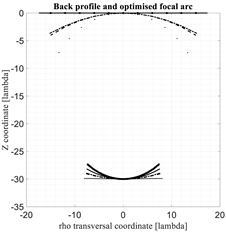
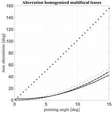
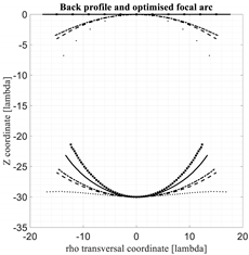
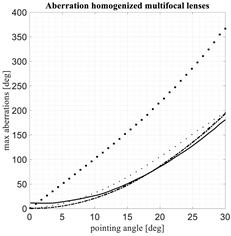
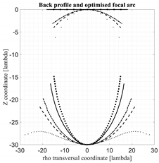
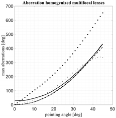
In

Table 1. M = zooming = 1.

$\mathsf{\alpha }=15°$
$\mathsf{\alpha }=30°$
$\mathsf{\alpha }=45°$

, these five lens architectures are compared. First of all, the shape of the back lens and the shape of the optimized focal arcs are plotted in the left part of the Table. The front lens is not visualized because all the architectures compared in this section are characterized by a flat profile. As is well known, by reducing the curvature of the back lens, the curvature of the corresponding optimized focal arc increases. However, a further important property can be appreciated: small variations in the back lens curvature imply significant variations in the corresponding focal arcs. The shapes of the back lenses and homologous focal arcs are useful also to estimate the accommodation constraints and to have a first idea of the coupling coefficients between the focal arc and the back lens. Second, the aberrations of the homogenized rotationally symmetric lenses are presented in the right part of Table 1.

In particular, the results relevant to the spherical-planar lens are represented by dashed lines, the results of the McGrath lens by square points, the results of the Sole and Smith lens by dotted lines, the results of the three-foci lens by continuous lines, the results of the four-foci lens by dotted-dashed lines. Out of these five architectures only the first one, the spherical-planar lens, is rotationally symmetric. The other ones have been homogenized (by transforming them into rotationally symmetric lenses) in order to improve their performance and to improve their manufacturability. In Table 1, the case of a lens with front diameter equal to 30λ is considered; the magnification M = 1.

Three opening angles are considered: $\mathsf{\alpha }=15°,30°,45°$. In order to have a fair comparison, the configurations are compared by enforcing that their optimized focal length along the axis are equal or extremely similar. This condition is important to have architectures with similar accommodation constraints. Accordingly, in Table 1 the axial focal distance has a value close to the diameter of the front lens, i.e., 30λ.

In general, the symmetrized Sole and Smith lens (results in dotted lines) exhibits always the flattest focal curve and the most curved back lens profile. The McGrath lens (results in squared dots) exhibits the most curved focal profile and the worst aberrations. The four-foci lens and the spherical-planar lens, once optimized, present extremely similar results. Actually, for $\mathsf{\alpha }=15°$ the optimized focal curves for these two lenses are practically overlapped and also the back profiles are extremely similar.

The two lenses with both back and front profiles flat, i.e., the McGrath lens and the new three-foci lens, offer some simplifications in terms of manufacturability associated to the planarity of both profiles. Out of these two lenses the new lens with three foci, after enforcing the rotational symmetry, provide significantly better aberrations as compared to the optimized McGrath lens. It exhibits some residual aberrations on the lens axis (this is not a surprise considering this lens does not have any axial focus), but having the three foci out of the axis permits to better control the aberrations when the scanning angle increases. The Sole and Smith lens, after enforcing the rotational symmetry, exhibits the best aberrations for $\mathsf{\alpha }=45°$. However, the corresponding optimized focal arc, as evident looking at the results for $\mathsf{\alpha }=45°$, is characterized by a shape less convenient to guarantee a good illumination of the lens from the focal arc.

Overall, the lens architectures which at the same time offer good aberrations vs. scanning, and a free-space cavity (delimited by the back lens and the focal arc) as similar as possible to a sphere, are the spherical-planar lens with a single axial focus, and the four-foci lens with flat front profile, back profile like a saddle, elements aligned radially, F = G, α ≠ δ.

It is important to observe that a conversion from a spherical wave into a plane wave is more naturally achieved using a curved back profile (similar to the impinging spherical front phase) and a flat front profile (similar to the desired final plane wave). In the two lenses with flat back and front profiles, i.e., the McGrath lens and the new three-foci lens, the enforced planarity of both profiles guarantee some cost reduction but it is counterbalanced by the fact that the positions of homologous elements follow a quite nonlinear law so the accommodation and cost of corresponding transmission lines increase. In addition, the lenses with flat back profile require a longer focal distances to achieve comparable aberrations. Overall, in terms of cost, manufacturability and accommodation constraints, lenses with a flat front profile and a curved back profile similar to a spherical profile represent a suitable solution.

It is important to provide some considerations on the aberrations as a function of the magnification factor M. For a fixed dimension of the front lens and a fixed maximum scanning of the feeding array illuminating the back lens, aberrations are directly proportional to the Zooming factor. If one reduces the back lens dimensions by a linear factor of two (i.e., M = 0.5), one may expect a saving factor of eight in terms of volume, a scanning domain reduced by a factor of two (or better a factor two in terms of the sine of the scanning angle), and a saving factor of two in the aberrations. Vice versa, if one increases the back lens dimensions by a linear factor of two (i.e., M = 2), one may expect an increase by a factor of eight in terms of volume, a scanning domain magnified by a factor of two (or better a factor of two in terms of the sine of the scanning angle), and an increase by a factor two in the aberrations. The corresponding profiles and curves in case of magnification factor smaller or larger than one are not presented because, except for this described scaling factor, remain practically identical as compared to the ones reported in Table 1.

The considerations reported in this paper are valid for lenses such that the distance between the last feed (the one scanning the maximum angle versus the lens axis) as compared to the axis is smaller than the back lens radius. Lenses with larger field of view, such that the distance between the last feed as compared to the axis is larger than the back lens radius, are investigated in the part III companion paper.

9. Conclusions

Several new three-dimensional discrete constrained lenses characterized by one, three, four and five focal points have been introduced in this paper. Bifocal lenses, i.e., lenses characterized by two focal points, have not been considered here. One possible bifocal lens is presented in [28]; it can be considered a transmit array because the back and front profile coincide and it has homologous elements in the back and front lens. This bifocal lens has two degrees of freedom only (associated to the profile and to the phase) and two perfect focal points.

An innovative numerical procedure to homogenize lenses that are not rotationally symmetric has been proposed with two main objectives: reducing the maximum aberrations and significantly improving the lens manufacturing. In addition, a new rigorous algorithm to define the focal surface that allows to guarantee minimum aberrations has been introduced. A property already well known in the literature has been confirmed: reducing the curvature of the back lens profile implies that the optimized focal arc results in being more curved, and vice versa.

The new three-foci lens proposed exhibits aberrations significantly improved as compared to the McGrath lens (characterized as well by two flat profiles). In particular, for lenses characterized by a limited field of view, the reduction in the aberrations is close to a factor of three. At the same time this lens guarantees a simple manufacturability of the back and front lenses.

The new four-foci lens—with flat front profile, back profile like a saddle, elements radially aligned, F = G, α ≠ δ after homogenization and after optimizing the focal arc—presents performance similar to the spherical-planar lens with a single axial focus.

As a result of the comparison between different 3D multifocal discrete lenses, two lens architectures appear to offer particularly good performance: the new three-foci lens with flat back and front profile, and the new four-foci lens behaving similarly as compared to the spherical-planar single focus lens.

It is interesting to note that in the limit case where the back and front elements of the lens are collocated the discrete lens can be considered a transmit array or metalens. Some properties of metamaterial transmission-line based antennas are presented in [29].

All the lens architectures presented in the paper have been obtained solving geometrical optics (GO) equations with the symbolic tool MUPAD available in Matlab [30]. The focal arcs have been optimized adopting min-max analytical/numerical approaches in order to minimize the maximum optical aberration for every scanning angle. The results presented provide useful indications for the preliminary design of constrained lens antennas before adopting full wave rigorous techniques.