Abstract
In this paper, an innovative procedure is proposed for the design of three-dimensional discrete lens antennas characterized by an extended field of view. While in a companion paper the design procedure was based on the definition of multifocal constrained lenses and on their evolution in rotationally symmetric ones, in this paper, lenses are assumed from the beginning to be rotationally symmetric and are derived by enforcing minimized optical aberrations specifically for the largest scanning directions. It is shown that, for discrete lenses exhibiting a feeding array with a cross section, projected in a plane perpendicular to the main lens axis, larger as compared to the back lens cross section, there are significant improvements (15–20%) in terms of maximum aberrations and, at the same time, similar or slightly improved accommodation in terms of volume can be obtained as compared to the architectures considered in the companion paper. Because of this property, the proposed lens antennas may be particularly useful in emerging applications requiring an extended field of view.
1. Introduction
Discrete lens beamforming networks (BFNs) and antennas are also known as bootlace lenses, constrained lenses, or discretized array lenses [1,2]. Three-dimensional lenses have been investigated less as compared to two-dimensional ones. In [3], J.B.L. Rao investigated three-dimensional bootlace lenses having two, three, and four perfect focal points located in a single plane containing the longitudinal axis of the lens. The results of the aperture phase error analysis showed that a lens with a larger number of focal points can be scanned to much larger angles in one plane at the expense of the scanning capability in the orthogonal plane. J.L. McFarland and J.S. Ajioka [4] have proposed a bispherical lens, composed by two portions of spheres with two identical radii, for three-dimensional scanning. J.B.L. Rao [5] generalized this bispherical lens to include two spheres with different radii in order to control the accommodation of the lens. McGrath [6] has introduced a simple three-dimensional lens with flat front and back profiles, homologous elements aligned radially and exhibiting two superimposed foci located in the lens axis. Immediately after, Sole and Smith [7] introduced a three-dimensional lens with a flat front profile, back profile with the shape of a saddle, and four focal points. They showed that similar performance in terms of optical aberrations as compared to the McGrath lens can be obtained adopting a more compact lens with a curved back profile. C. Rappaport and A. Zaghloul [8] have also studied three-dimensional lenses having two, three, and four focal points located in a plane containing the longitudinal axis of the lens so only able to perform a two-dimensional type of scanning. C. Rappaport and J. Mason [9] have considered a five-foci three dimensional discrete lens; however, only a limited numerical investigation was proposed.
It is important to note that a three-dimensional scanning can be obtained also by cascading two blocks of two-dimensional bootlace lenses as conducted at Raytheon by Maybell and colleagues [10,11] and by Chan, Rao and Bhattacharyya in [12,13].
In the last 15 years, several developments on three-dimensional constrained lenses have been initiated by the European Space Agency [14,15,16,17,18,19,20]. In [16,17,18,19,20], in order to improve the transfer of power within the lens and to better control the amplitude tapering and sidelobe level, radiating elements characterized by different apertures have been exploited. In [20], a three-dimensional constrained lens able to operate both in transmission and reception was proposed for the first time.
The objective of this paper is the present a new type of afocal lenses optimized for large scanning angles. This work can be considered an extension of the work published in a companion paper [2]. In particular, discrete lenses exhibiting a feeding array with a cross section, projected in a plane perpendicular to the main lens axis, larger as compared to the back lens cross section are primarily considered in this paper. In this condition, where severe optical aberrations are experienced, it will be shown that the results previously presented on three-dimensional discrete lens antennas can be further improved. Two significant improvements are obtained and discussed: a reduction in the optical aberrations and a reduction in the optimized focal distances with an improvement in terms of accommodation.
2. Enforcing a Chebyshev-Like Condition for the Maximum Aberrations on the Rim of the Lens
The new lens formulation is derived starting from the following consideration: the maximum aberrations for an arbitrary pointing angle are typically associated with the most peripheral points of the lens. Because of this property, generally valid for rotationally symmetric 3D lenses, the attention can be focused on the evolutions of maximum aberrations along the external rim of the three-dimensional lens. The external rim, being the lens rotationally symmetric, can be considered circular.
Let us consider an example with unitary zooming factor (i.e., M = 1), maximum scanning angle 60°, diameter of the front lens equal to 30 wavelengths, as in the several examples presented in [1,2]. When considering large scanning angles, such as 60°, the differences in performance between various lenses, such as the ones defined in [1,2], tend to be large so it is useful to focus the attention on this type of large scanning trying to possibly improve the performance achievable with multifocal bootlace lenses. Let us assume that the feeding point is located in a point characterized by the following Cartesian coordinates expressed in wavelengths: (30 sin(60°), 0, −30 cos(60°)). The three-foci constrained lens with flat back and front profile presented in [1,2] is considered in this case, but similar properties are valid for different configurations. In Figure 1, the optical aberrations (expressed in degrees) evaluated when illuminating only the peripheral rim of the back lens are plotted. In the abscise axis, the azimuthal angle ranging from 0° to 360° is shown.
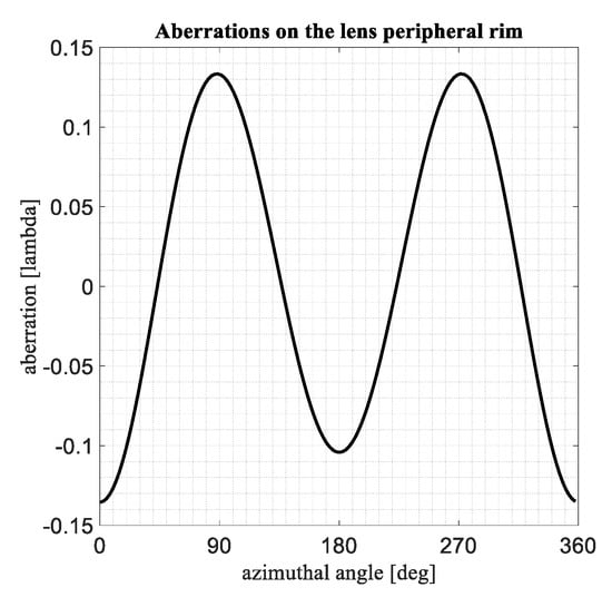
Figure 1.
Typical optical aberrations evaluated on the peripheral rim of the lens as a function of the azimuthal angle.
Real instead of absolute values are plotted in order to better visualize the evolutions of the aberrations. The curve exhibits a sort of sinusoidal behavior. However, the maximum and the minimum values, in absolute value, are similar but not identical. This is not a surprise: in fact, the source illuminating the lenses is not located on the central axis (a skew incidence condition is considered) so there is no reason to obtain aberrations along the rim exhibiting identical maximum and minimum values. Certainly, the values obtained when the azimuth ranges from 0° to 180° coincide with the ones obtained when the azimuth ranges from 180° to 360°.
Starting from the previous considerations, a new strategy to define 3D discrete lenses has been conceived. Let us fix the position of the feed in the point with the Cartesian coordinates:
where, as in [2], sa = sin(α), ca = cos(α) and α is the maximum scanning angle of the lens.
Indicating with the maximum radius of the back lens and1 the maximum radius of the front lens, and assuming the lens rotationally symmetric, the following relations are valid:
The feeding point is considered fixed, as the maximum scanning angle α and the maximum radius of the front lens R1. The unknowns of the lens are R, Z, W and Z1. Let us write the aberrations in an arbitrary point of the external rim of the lens:
Let us in this case define also:
Thus, the aberrations in φ = 0° are forced to be identical in absolute value, but with an opposite sign, as compared to the aberrations in φ = 90°. As a second equation, the aberrations in φ = 90° are assumed to be identical in absolute value, but with opposite sign, as compared to the aberrations for φ = 180°. These two equations permit forcing the aberrations on the lens rim to have identical positive and negative maximum excursions. This represents a locally optimum condition. In fact, when deviating from this condition, neither the positive aberrations nor the negative become dominant with an overall increase in the absolute value of the maximum aberrations.
The 3D lens has in general 5 degrees of freedom. These are reduced to 4 when enforcing the rotational symmetry. One additional degree of freedom can be spent in enforcing the front profile of the lens to be flat. After these two assumptions, three quantities remain unknowns: Z, W, and R, i.e., the rotationally symmetric profile of the back lens, the phase shifts W, and the relation between the radial coordinate R1 in the front lens (assumed to be known) and the corresponding radial coordinate R in the back lens aperture. By enforcing the two additional conditions corresponding to the two properties described, two new equations are available:
so that two of the three unknowns can be derived. The third unknown can be fixed a priori. At least three choices are available:
- (a)
- The Z is fixed in advance, for instance a spherical, or ellipsoidal, back profile can be selected;
- (b)
- The W is fixed in advance, for instance the choice W = 0 can be performed in order to guarantee that all the transmission lines are equi-length;
- (c)
- The R is fixed, for instance R = R1 M in order to guarantee a regular distribution and density of the elements. Another possibility is to enforce that the elements in the front and back lens (in the case of unitary zooming, i.e., M = 1) are aligned along straight lines originated not at an infinite distance, but in a point at a finite distance along the lens axis (as performed, for the R-2R two-dimensional lens).
The fundamental result is the following: by enforcing the two previous equations, the results obtained in the previous paper [2], when comparing different types of lenses, can be further improved when considering focal surfaces with a diameter exceeding the diameter of the back lens. This condition is achieved typically for lenses characterized by a large field of view (i.e., larger than 40°). It will be shown that is possible to reduce further the optical aberrations and, at the same time, to reduce the length of the focal distances. It is important to note that we do not enforce any perfect focal point when enforcing the two last equations. The two conditions are only enforced in the circular peripheral rim of the lens representing the most critical part of the lens in terms of optical aberrations. However, the two innovative conditions introduced in this paper for the first time guarantee the presence as well of four points in the rim of the lens where the aberrations assume a zero value. These four points are located close to the angles φ = 45°, 135°, 225°, and 315°, but not exactly in these 4 angles.
The analytical results are presented below:
- (a)
- By solving the two Equations (1a,b) using R and W as unknowns, four solutions are found, the acceptable ones being the following:As a limit case, by forcing both Z1 and Z to be null:
- (b)
- By solving the two Equation (1a,b) using R and Z as unknowns, after enforcing Z1 = 0 and W = 0 (i.e., equi-length transmission lines), four solutions are found. The acceptable ones are the following:
- (c)
- By solving the two Equation (1a,b) using W and Z as unknowns, after enforcing Z1 = 0 and fixing R (for instance R = R1 M), four solutions are found, the acceptable ones being the following:
3. An Improved Formulation
A further improvement is proposed in this section. Let us first represent the aberrations on the entire surface of the lens, still maintaining the source fixed in the same position corresponding to the maximum scanning angle. Their typical behavior is shown in Figure 2. As evident, the aberrations exhibit a saddle shape. Two quadratic curves with opposite curvatures appear in the two principal perpendicular planes. In particular, the saddle is slightly tilted towards the direction of the source (see picture on the right). Because of this small tilt, the aberrations with maximum value and positive sign are obtained in the rim not exactly in correspondence to the angle φ = 90°, but for a slightly smaller angle. This point on the rim can be derived with the following hypothesis. Again, we consider the feed fixed in the plane phi = 0° and the transversal coordinates expressed as:
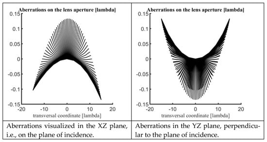
Figure 2.
Typical evolutions of the aberrations on the lens aperture illuminated with the maximum scanning angle.
The Cartesian coordinates of the feeding point are:
It was verified that the point on the rim where the aberrations assume a maximum positive value can be derived enforcing that, in this point, the radial vector with components X and Y is perpendicular to the incident field. The scalar product between these two vectors is given by:
By enforcing a null scalar product, the following condition is derived:
The other two points where the aberrations assume the minimum real values do not change as compared to the previous derivation. They are located in the principal plane containing the source and they are characterized by φ = 0° and 180°.
By enforcing now the two conditions:
and using the value for derived in (2), four solutions are obtained.
In particular, by solving the two conditions in (3a) and (3b), the acceptable solution is the following:
Because two conditions were enforced and there are four unknowns, the solutions remain expressed as a function of two parameters, p and q. In particular, the expression Z1 = q tell us that the Z1, i.e., the front profile, is undetermined. A common choice is to fix it to be null. We have already seen in [1,2] that the aberrations are mainly determined by the back profile shape Z and having a Z1 different from zero implies larger volume and higher cost in terms of manufacturability. So, choosing q = 0, implying Z1 = 0 results to be a suitable assumption. The p value can be easily derived enforcing another condition.
A. By solving for W and R (so assuming Z1 and Z assigned)
In this case, one derives four solutions. The acceptable one is:
Possible choices for the profile Z may be spherical, paraboloidal, ellipsoidal, etc. Fixing Z1 = 0 and selecting a priori different types of back profiles Z give a significant flexibility. Several investigations have been conducted using profiles with both types of convexity. In the end, to optimize the coupling between the feeds and the back lens as well, a rotationally symmetric concave back profile with the concavity in the direction of the focal arc represents a good choice.
B. By solving for Z and R (so assuming Z1 and W assigned)
In this case, one derives four solutions. In the general case of Z1 and W being different from zero, the analytical expressions are extremely cumbersome. The most convenient configurations are characterized by a flat front profile, so assuming Z1 = 0 does not represent a limitation. By assuming Z1 = 0 and W = 0 (equi-length lines), the expressions are significantly simplified:
C. By solving for Z and W (so assuming Z1 and R assigned)
In this case, one derives four solutions. The acceptable one is:
D. By enforcing
This represents another interesting case:
with n real, i.e., the phase path proportional to the physical distance between homologous points. The proportionality factor, n, is used in analogy with the dielectric lenses where n represents the refractive index of the dielectric material (n for dielectric lenses = sqrt(dielectric constant)). This case is important because the lines connecting homologous points can be straight lines and the type of connecting lines (i.e., coaxial cables, fiber optics, waveguides, etc.) characterizes the proportionality factor n. It is important to mention that, while for dielectric lenses the factor n is typically larger than 1, and dielectric lenses tend to be thicker at the center and thinner at the periphery, the contrary is valid for microwave lenses where the connecting lines are constituted by coaxial cables, waveguides or other similar passive microwave components. In constrained lenses, the factor n is typically smaller than 1 and these lenses exhibit a minimum thickness at the center and a maximum one on the periphery.
Four possibilities were identified. The corresponding solutions are reported in Table 1. Two possibilities were obtained by enforcing Equations (2) and (3), the other two possibilities simply enforcing the presence of a single focal point in the lens axis located in the point with Cartesian coordinates (−H,0,0).

Table 1.
Lenses with phase shifters W proportional to the distance of homologous points.
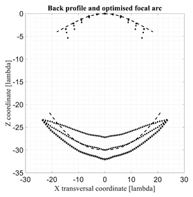
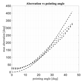
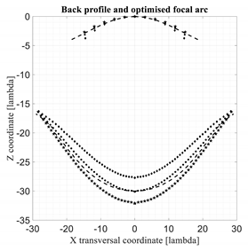
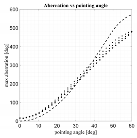
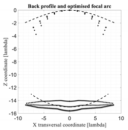
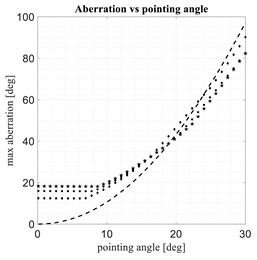
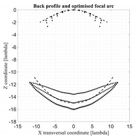
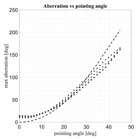
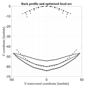
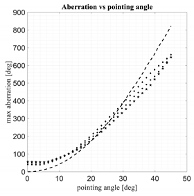
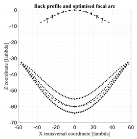
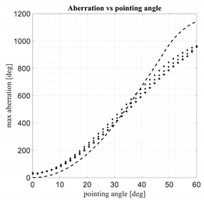
4. Numerical Results
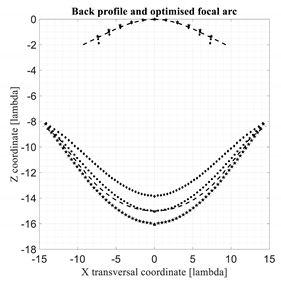
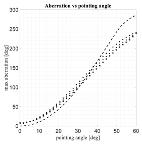
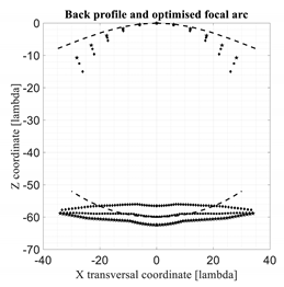
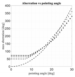
As anticipated in the previous sections and in [1,2], the profile of the back lens plays a fundamental role in defining the shape of the optimized focal arc and the behavior of the maximum aberrations. In this section, the performance of the spherical–planar bootlace lens, defined and discussed in [1,2], characterized by a single axial focus located in the point (0,0,−R0), is compared to the performance of three constrained lenses with Z and Z1 assigned (with a flat front profile, i.e., Z1 = 0) and W and R obtained by solving (2) and (3) and defined in (4). The three profiles for the back lens are paraboloidal profiles defined by:
With the parameter A:
where D represents the diameter of the front lens and M is the magnification factor. In addition, the parameter F for the three paraboloidal lenses is related to the radius R0 of the spherical–planar lens by these heuristic expressions:
F = 0.905 R0 for α = 30°; F = 0.818 R0 for α = 45°; F = 0.7435 R0 for α = 60°;
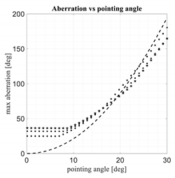
The heuristic values in (5) and (6) were derived in order to have the three paraboloidal lenses with axial focal distances comparable with the one of the spherical–planar one. The results of this comparison are presented in Table 2. The curves relevant to the three paraboloidal lenses are represented with diamond, circle and star points. In particular, the paraboloidal lenses characterized by the smallest values of the A parameter are represented with the star points, the ones characterized by the largest values of the A parameter are represented with the diamond points, while for the intermediate A parameters circles are used.
Table 2.
Comparison between 3D discrete lenses. M = zooming = 1.
For the three new lenses exhibit moderate improvements in the maximum aberrations for angles close to the maximum one. Close to the axis, these three lenses are not able to minimize the aberrations, but these values are much less critical. The results of the three lenses in terms of aberrations when approaching the lens axis are not surprising because their performance was optimized only for the maximum scanning angle where the most critical values are obtained.
For the three new lenses exhibit significant improvements in terms of aberrations (in the order of 20%) as compared to the spherical–planar lens, while they are comparable in terms of focal distances so in terms of accommodation constraints.
It is important to note that this type of lenses may be used to scan approximately up to when the axial focal is comparable with the lens diameter. For larger scanning angles, the illumination efficiency associated with the peripheral feeds is becoming poor.
In Table 3 and Table 4 the same results proposed in Table 2 are evaluated for con-strained lenses characterized by a zooming factor equal to 0.5 and 2.
Table 3.
Comparison between 3D discrete lenses. M = zooming = 0.5.
Table 4.
Comparison between 3D discrete lenses. M = zooming = 2.
5. Conclusions
A design procedure to derive rotationally symmetric three-dimensional lenses with large field of view and minimized optical aberrations was proposed. A reduction in the order of 20% in the maximum aberrations was found as compared to the case of multifocal three-dimensional lenses properly symmetrized. The new architectures offer improved performance also in terms of accommodation because they allow reducing the focal lengths. The improvements are valid for lens antennas characterized by focal feeding arrays with a diameter exceeding the back lens diameter. It is interesting to note that, when this condition applies, the aberrations remain lower as compared to the ones of comparable multifocal lenses for all the scanning angles higher than about half the maximum scanning angle, while their values are higher in the first half of the scanning region starting from the lens axis. The design procedure may be useful to define bootlace lens antennas operating in several emerging applications (i.e., Space, 5G, MIMO, etc).
Author Contributions
Methodology, G.T. and P.A.; software, G.T. and P.A.; validation, G.T. and P.A.; writing—original draft preparation, G.T. and P.A.; writing—review and editing, G.T. and P.A. All authors have read and agreed to the published version of the manuscript.
Funding
This research received no external funding.
Institutional Review Board Statement
Not applicable.
Informed Consent Statement
Not applicable.
Conflicts of Interest
The authors declare no conflict of interest.
References
- Toso, G.; Angeletti, P. Two-Dimensional and Three-Dimensional Discrete Constrained Lenses with Minimised Optical Aberrations. International Patent Application No. PCT/EP2021/052202, 29 January 2021. [Google Scholar]
- Toso, G.; Angeletti, P. An Optimal Procedure for the Design of Discrete Constrained Lens Antennas with Minimized Optical Aberrations. Part II: Three-Dimensional Multifocal Architectures. Electronics 2022, 11, 503. [Google Scholar] [CrossRef]
- Rao, J.B.L. Multifocal Three-Dimensional Bootlace Lenses. IEEE Trans. Antennas Propag. 1982, 30, 1050–1056. [Google Scholar] [CrossRef]
- McFarland, J.L.; Ajioka, J.S. Multiple-beam constrained lens. Microwaves 1963, 2, 81–89. [Google Scholar]
- Rao, J.B.L. Bispherical constrained lens antenna. IEEE Trans. Antennas Propag. 1986, 30, 1224–1228. [Google Scholar] [CrossRef]
- McGrath, D.T. Planar Three-Dimensional constrained lenses. IEEE Trans. Antennas Propag. 1986, 34, 46–50. [Google Scholar] [CrossRef] [Green Version]
- Sole, G.C.; Smith, M.S. Multiple beam forming for planar antenna arrays using a three-dimensional Rotman lens. In IEE Proceedings H (Microwaves, Antennas and Propagation); IET Digital Library: Hoboken, NJ, USA, 1987; pp. 375–385. [Google Scholar]
- Rappaport, C.M.; Zaghloul, A. Optimized Three Dimensional Lenses for Wide-Angle Two Dimensional Scanning. IEEE Trans. Antennas Propag. 1985, 33, 1227–1236. [Google Scholar] [CrossRef]
- Rappaport, C.M.; Mason, J. A five focal point three-dimensional bootlace lens with scanning in two planes. In Proceedings of the IEEE Antennas and Propagation Society International Symposium, Chicago, IL, USA, 18–25 June 1992. [Google Scholar]
- Archer, D.H.; Maybell, M.J. Rotman lens development history at Raytheon Electronic Warfare Systems 1967–1995. In Proceedings of the 2005 IEEE Antennas and Propagation Society International Symposium, Washington, DC, USA, 3–8 July 2005. [Google Scholar]
- Maybell, M.J.; Chan, K.K.; Simon, P.S. Rotman lens recent developments 1994–2005. In Proceedings of the 2005 IEEE Anten-nas and Propagation Society International Symposium, Washington, DC, USA, 3–8 July 2005. [Google Scholar]
- Chan, K.K.; Rao, S.K. Design of a Rotman lens feed network to generate a hexagonal lattice of multiple beams. IEEE Trans. Antennas Propag. 2002, 50, 1099–1108. [Google Scholar] [CrossRef]
- Rao, S.K.; Bhattacharyya, A.K. Low Cost Space-Fed Reconfigurable Phased Array for Spacecraft and Aircraft Applications. U.S. Patent 2016/0248157 A1, 25 August 2016. [Google Scholar]
- Toso, G.; Angeletti, P.; Ruggerini, G.; Bellaveglia, G. Multibeam Active Discrete Lens Antenna. US Patent 8,358,249, 22 January 2013. [Google Scholar]
- Trastoy, A.; Montesano, A.; Campuzano, J.; Bustamante, M.; Alvarez, D.; Martin-Polegre, A. Lens-based DRA Ka Band Transmission Antenna. Design and DM Testing. In Proceedings of the 2nd ESA Workshop on Advanced Flexible Telecom Payloads, Noordwijk, The Netherlands, 17–19 April 2012. [Google Scholar]
- Ruggerini, G.; Nicolaci, P.G.; Toso, G.; Angeletti, P. A Ka-Band Active Aperiodic Constrained Lens Antenna for Multibeam Applications. IEEE Antennas Propag. Mag. 2019, 61, 60–68. [Google Scholar] [CrossRef]
- Angeletti, P.; Toso, G.; Ruggerini, G. Array Antenna with Optimized Elements Positions and Dimensions. International Patent WO2014114993 A1, 31 July 2014. [Google Scholar]
- Angeletti, P.; Toso, G.; Ruggerini, G. Array Antennas with Jointly Optimized Elements Positions and Dimensions Part II: Planar Circular Arrays. IEEE Trans. Antennas Propag. 2013, 62, 1627–1639. [Google Scholar] [CrossRef]
- Ruggerini, G.; Nicolaci, P.; Toso, G.; Angeletti, P. An active discrete lens antenna for Ka-band multibeam applications. In Proceedings of the 2012 IEEE International Symposium on Antennas and Propagation, Chicago, IL, USA, 8–14 July 2012. [Google Scholar]
- Ruggerini, G.; Nicolaci, P.G.; Toso, G. A Ku-Band Magnified Active Tx/Rx Multibeam Antenna Based on a Discrete Con-strained Lens. Electronics 2021, 10, 2824. [Google Scholar] [CrossRef]
Publisher’s Note: MDPI stays neutral with regard to jurisdictional claims in published maps and institutional affiliations. |
© 2022 by the authors. Licensee MDPI, Basel, Switzerland. This article is an open access article distributed under the terms and conditions of the Creative Commons Attribution (CC BY) license (https://creativecommons.org/licenses/by/4.0/).