Diagnosis Myocardial Infarction Based on Stacking Ensemble of Convolutional Neural Network

Abstract

Artificial Intelligence (AI) technologies are vital in identifying patients at risk of serious illness by providing an early hazards risk. Myocardial infarction (MI) is a silent disease that has been harvested and is still threatening many lives. The aim of this work is to propose a stacking ensemble based on Convolutional Neural Network model (CNN). The proposed model consists of two primary levels, Level-1 and Level-2. In Level-1, the pre-trained CNN models (i.e., CNN-Model1, CNN-Model2, and CNN-Model3) produce the output probabilities and collect them in stacking for the training and testing sets. In Level-2, four meta-leaner classifiers (i.e., SVM, LR, RF, or KNN) are trained by stacking the output probabilities of the training set and are evaluated using the stacking of the output probabilities of the testing set to make the final prediction results. The proposed work was evaluated based on two ECG heartbeat signals datasets for MI: Massachusetts Institute of Technology-Beth Israel Hospital (MIT-BIH) and Physikalisch-Technische Bundesanstalt (PTB) datasets. The proposed model was compared with a diverse set of classical machine learning algorithms such as decision tree, K-nearest neighbor, and support vector machine, and the three base CNN classifiers of CNN-Model1, CNN-Model2, and CNN-Model3. The proposed model based on the RF meta-learner classifier obtained the highest scores, achieving remarkable results on both databases used. For the MIT-BIH dataset it achieved an accuracy of 99.8%, precision of 97%, recall of 96%, and F1-score of 94.4%, outperforming all other methods. while with PTB dataset achieved an accuracy of 99.7%, precision of 99%, recall of 99%, and F1-score of 99%, exceeding the other methods.

1. Introduction

A myocardial infarction (MI) happens if one or even more segments of the heart muscle stop receiving adequate oxygen. MI happens when blood flow to the heart muscle is restricted or obstructed. In the United States, a heart attack occurs every 40 s, and approximately 805,000 people experience a heart attack every year [1,2]. People frequently confuse myocardial infarction for less severe cases, minimizing the issue and failing to give it the attention it deserves. The indications of a MI are so subtle and transient that individuals dismiss them as normal pain or a small ailment of another sort [3]. MI causes discomfort in the middle of the chest instead of severe pain on the left side, which many associates with heart attacks. Patients might still believe they are normal during and after a silent MI, increasing the probability that warning symptoms may be disregarded [4].

A physician’s first step in MI treatment is diagnosis, which has to be fast and accurate to save the patients’ lives. Coronary angiography imaging is applied to study the blood veins in the heart by generating pictures revealing the problems with the blood vessels. The test is often used to assess whether or not there is a blockage in blood flow to the heart. Electrocardiogram (ECG) is also used to capture electrical impulses in the heart. Secondly, there is the treatment process for improving the blood flow to the heart muscle. The doctor may offer medication, surgery, or both. A catheter (a long, thin tube) is put into the restricted segment of the artery, which may be useful for widening the artery. A thin wire mesh coil (stent) is routinely used to keep the artery open. A graft is produced by a surgeon utilizing a vascular from another part of the patient’s body to allow blood to flow past the blocked or restricted coronary artery [5,6].

The seriousness of a myocardial infarction disease is increased, and its symptoms are similar to other symptoms that may appear to the patient as normal symptoms, contributing to the delay in diagnosis and appropriate treatment. It is necessary to find accurate and definitive ways to identify myocardial infarction disease. In addition, early identifying patients at risk of MI can prevent permanent cardiac damage using electrocardiogram (ECG) data to automatically and accurately predict myocardial infarction (MI) for detecting and treating heart diseases. Artificial intelligence-based deep learning (DL) and machine learning (ML) methods have achieved great success in the medical analysis domain [7,8,9,10]. There are many available AI techniques that use deep convolutional neural network (CNN) for the following reasons. Deep CNNs’ numerous layers enable models to become more efficient at learning detailed information incrementally and executing more heavy computational tasks, and it can extract deep features from datasets [11,12].

Ensemble techniques are approaches that combine different learning algorithms or models to create a single, ideal prediction model that performs better than the base learners considered separately [13,14,15]. The ensemble learning method involves three different methods, the difference of which is centered on how the inputs are combined to obtain distinct outputs, namely stacking, boosting, and bagging [16]. Stacking considers heterogeneous vulnerable learners who proceed to learn the process in parallel and then combine them by training a meta-learner to gain a prediction based on the multiple vulnerable learners’ predictions [17,18]. The generalization capacity may be successfully improved by ensemble learning in both theory and practice [19]. Stacking differs from bagging and boosting in two ways. First, stacking considers heterogeneous weak learners (various learning algorithms are merged), whereas bagging and boosting mostly consider homogeneous weak learners [10,20]. Second, stacking uses a meta-model to combine the basic models, whereas bagging and boosting combine weak learners by using deterministic techniques [21], which aligns best with the proposed model in that research.

Maintaining public health has become a critical challenge and objective for health organizations around the world. Therefore, many studies have used ML, DL, and deep CNN [22,23,24] to identify patients at risk of MI and to find ways to help diagnose or cure MI diseases. Previous studies have used ML, CNN, and hybrid models to detect MI. In addition, they do not use stacking and ensemble based on different heterogeneous architectures of the CNN models. As a result, this the first time that stacking ensemble has been used for this disease. We proposed a stacking ensemble model that combined the three CNN base models of CNN-Model1, CNN-Model2, and CNN-Model3 with the meta-learner classifiers from SVM, RF, KNN, or LR to investigate the risk identification practices in critical healthcare use cases of MI.

Our contributions can be summarized as follows:

• Three optimized CNN models with heterogeneous architectures: CNN-Model1, CNN-Model2, and CNN-Model3. The Bayesian optimizer has been used to find the best CNN architectures. These three models were used as pre-trained base classifiers for our proposed ensemble model. The Bayesian optimizer has been used for selecting the suitable CNN architecture;
• The stacking ensemble model was proposed to combine the three CNN base models of CNN-Model1, CNN-Model2, and CNN-Model3 with the meta-learner classifiers from SVM, RF, KNN, or LR. The best meta-learner selection was based on the performance of the ensemble model;
• Two popular and well-known benchmark datasets have been used to test the performance of the proposed model and compare it with other deep learning and classical machine learning models;
• The proposed model has achieved the highest accuracy, precision, recall, and F1-score performance compared with the other models.

Our study is structured as follows: Section 2 describes related work that has applied ML and DL models to detect and predict MI. The recommended stages and the proposed model are presented in Section 3. In Section 4, the experimental results are outlined and discussed. The paper is wrapped up and concluded in Section 6.

2. Related Work

The authors used CNN models with a variety of layers to detect MI. For example, In Ref. [22], the authors proposed a 12-layer deep 1D CNN to classify the 5 classes of heartbeat types in the MIT-BIH Arrhythmia database. They compared their proposed model with RF, neural networks, and other CNN networks, and it achieved the highest performance. In Ref. [23], the authors introduced a seven-layer deep 1D CNN dedicated for categorization using a specific structure design and parameters established to perform automated classification and feature extraction on a huge volume of source raw noisy signals. The findings indicated that their proposed model performed the best. In Ref. [24], the authors used the MIT-BIH database to train and evaluate the CNN models. By altering the number of epochs, the CNN model was examined using different activation functions. From the result, the ELU activation function gave the best accuracy. In Ref. [25], the authors proposed a 1D CNN model consisting of the input layer, two convolution layers, two downsampling layers, and one full connection layer and output layer for the classification of five typical kinds of MI using MIT-BIH arrhythmia database. In Ref. [26], the authors designed a deep CNN model to categorize the ECG data as normal or MI. Three convolutional blocks made up of several 1D convolutional layers were present in the model. Optimization techniques based on focal loss are also used to deal with imbalanced data and to obtain high training accuracy. The result showed that their model achieved the highest performance. In Ref. [27], the authors presented a deep CNN model to detect MI in 12-lead ECG recording. They used 12-lead signals from the PTB diagnostic ECG database of 10 distinct MI forms. Their proposed model has achieved high performance in MI detection. In Ref. [28], the authors proposed CNN to detect normal and MI from ECG singles with noise and without noise. CNN achieved the highest average accuracy without noise removal, respectively.

Other authors used hybrid models based on CNN, recurrent neural network (RNN) gated recurrent unit (GRU), long short-term memory (LSTM), and Bidirectional LSTM (BiLSTM) to detect MI. For example, in Ref. [29], the authors suggested a model that combines 24-layer deep CNN and BiLSTM to extract the structural and time-sensitive characteristics of ECG data in depth. They used kernels such as 32, 64, and 128 to extract detailed features of the ECG signal. The result showed that deep CNN and BiLSTM achieved the highest performance. In Ref. [30], the authors presented a hybrid model based on CNN and GRU (CNN-GRU) to categorize five types of MI from the MIT-BIH arrhythmia database. The hybrid model consists of a convolution layer followed by six local feature extraction modules (LFEM), GRU, dense layer, and Softmax layer. CNN-GRU had the best performance, according to the results. In Ref. [31], the authors classified MI from the MIT-BIH arrhythmia dataset and presented a hybrid model based on CNN and LSTM. They used layer-based LSTM and CNN to extract the full features and study the relationships in ECG signals. The result showed that combining LSTM and CNN achieved the highest accuracy. In Ref. [32], the authors presented a model based on combined CNN and RNN for classifying ECG cardiac impulses. The combined CNN and RNN was trained and examined using the MIT-BIH dataset. The result showed that the combined CNN and RNN achieved the highest performance. In Ref. [33], the authors proposed a combined mode based on the SVM and CNN to classify five classes of MI using the MIT-BIH arrhythmia database. They compared different CNN models with combined CNN and SVM, and it achieved the highest accuracy. In Ref. [34], the authors proposed a combined model based on CNN and RNN to classify multiclasses from ECG records. In addition, they suggested CNN-LSTM decoding, which improved the performance of detecting the multiclass classification from ECG records. The result showed that CNN-LSTM achieved the highest performance compared to other models. In addition, other authors used ML, DL models to detect MI. For example, Annisa et al. [35] applied LSTM on the PTB dataset to the binary classification of MI and healthy control patients. The usage of hyperparameters enhances the LSTM architecture’s performance. In Ref. [36], the authors used SVM and ANN to classify an ECG signal as healthy or MI. The ECG signals were obtained from the PTB. The overall showed that the SVM performs better than ANN. In Ref. [37], the authors applied a back propagation neural network (BPNN), RF, DT, and least-squares SVM (LS-SVM) to detect MI using the PTB database. The LS-SVM classifier achieved the highest classification accuracy.

The previous studies used ML, CNN, and hybrid models to detect MI. Additionally, they did not use stacking and ensemble based on different heterogeneous architectures of the CNN models. We propose a stacking ensemble model that combines the three CNN base models of CNN-Model1, CNN-Model2, and CNN-Model3 with the meta-learner classifiers from SVM, RF, KNN, or LR to investigate the risk identification practices in critical healthcare use cases of MI. The best meta-learner will be selected based on the performance of the ensemble model.

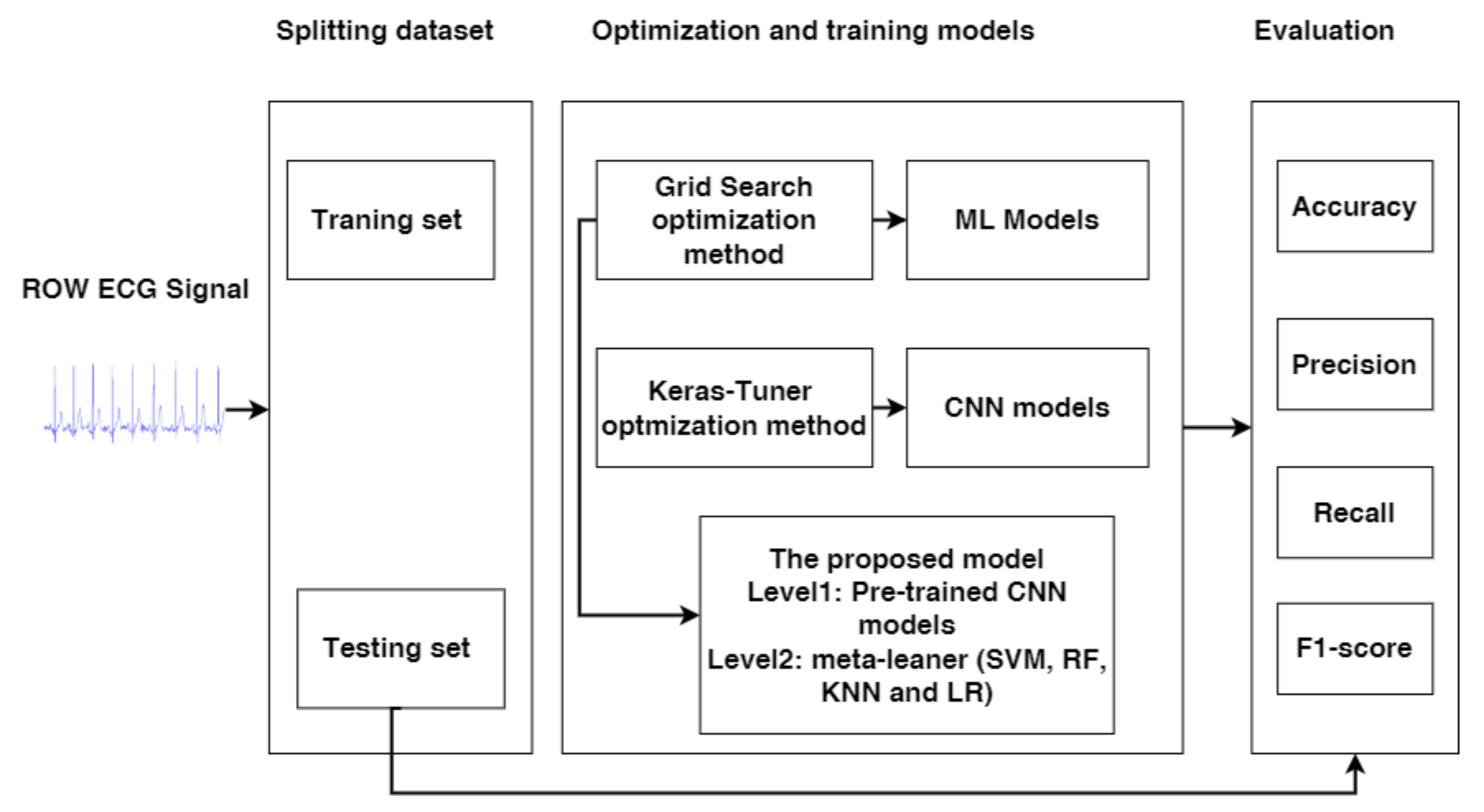
3. Methodology

In this work, we propose the stacking ensemble integrated pre-trained models CNN-Model1, CNN-Model2, and CNN-Model3 with four meta-learner classifiers SVM, RF, LR, and KNN. In addition, we propose models compared with the ML and CNN models. We will use optimization techniques to optimize the models, such as grid search for ML and meta-learner classifiers and Keras Tuner for CNN models. In addition, we will describe the complete processes that are applied for the prediction MI, as shown in Figure 1.

3.1. Datasets

Two ECG heartbeat signal datasets were used to conduct the experiments. The ECG heartbeat signals dataset is derived from two well-known datasets in heartbeat classification: MIT-BIH and PTB. Each dataset is made up of several CSV files. Each CSV file includes a matrix with a row for each sample in that particular dataset section. Each row’s last element identifies the class to which that example belongs.

• The first dataset is the MIT-BIH Arrhythmia dataset [38], which includes 109,446 samples and 5 classes: Normal (N), Article Premature(AP), Premature ventricular contraction(PVC), Fusion of ventricular and normal (FVN), and Fusion of paced and normal (FPN). MIT-BIH includes two CSV files: training and testing;
• The second dataset is the PTB Diagnostic ECG Database [38] with 14,552 subjects and 2 classes: normal and abnormal. The signals match the electrocardiogram (ECG) heartbeat patterns for healthy individuals and those suffering from arrhythmias and myocardial infarctions. These signals are refined and divided into segments, each of which represents a heartbeat. In addition, we divided PTB into an 80% training set and 20% testing set using stratified split methods.

Table 1. The number of subjects for the MIT-BIH and PTB datasets.

Datasets	Classes	Training Set	Testing Set
MIT-BIH dataset	N	72,471	18,117
	AP	6431	556
	PVC	5788	1448
	FVN	2223	162
	FPN	641	1608
	Total	87,554	21,892
PTB dataset	Recovered	198	52
	Death	88	20
	Total	286	72

presents the number of subjects for each class in two datasets for MIT-BIH and PTB, respectively.

3.2. Machine Learning Approach

We used different ML models: SVM, KNN, RF, and DT models, and they were optimized by grid search and cross-validation. We will describe the ML models, grid search, and cross-validation as follows.

3.2.1. ML Models

• SVM represents a supervised learning model that examines the data used for regression and classification analysis. The SVM algorithm [39] looks for the optimum hyperplane with the largest margin across classes in the n-dimensional classification space [40];
• K-Nearest Neighbor (KNN) is a learning technique used to identify and classify objects based on their nearest training samples in the feature space. By a majority vote of its neighbors, an object is assigned to the class that shares the same features with the majority of its k-nearest neighbors, where k is a positive integer [41];
• Decision tree (DT) is a ML algorithm that excels at grouping data elements into a structure resembling a tree. It compares the results for assorting data items into a tree structure to classifying and filtering options to help users make the best choices. DT has several levels, starting with the root node [42,43]. Each internal node represents a test for an input property or variable and has at least one child;
• Random Forest (RF) Algorithm is a type of supervised machine learning algorithm that is utilized to handle classification and regression situations [44]. It is typically used to solve classification issues by taking the majority vote or regression problems by finding the average of the input samples [45]. The basic goal of an RF tree is to employ a learning method to combine many weak learners into a single effective and robust predictor in order to categorize a new item based on its features. RF is made up of many trees, and the more trees there are, the sturdier it is [46].

3.2.2. Optimization Methods for the ML Models

• Grid search is a technique for hyperparameter tuning based on creating discrete grids by dividing the hyperparameter domain. Each combination of values in this grid is tested, and various performance metrics using cross-validation are determined in order to discover the grid point that maximizes the average value in cross-validation [47]; In contrast to other search techniques such as random search, grid search spans all the potential combinations to obtain the domain’s optimal point [48].
• Cross-validation: The training data was divided into K-folds in the same manner as K-fold cross-validation. The Kth part is then predicted using a basic model that was fitted to the K-1 parts.

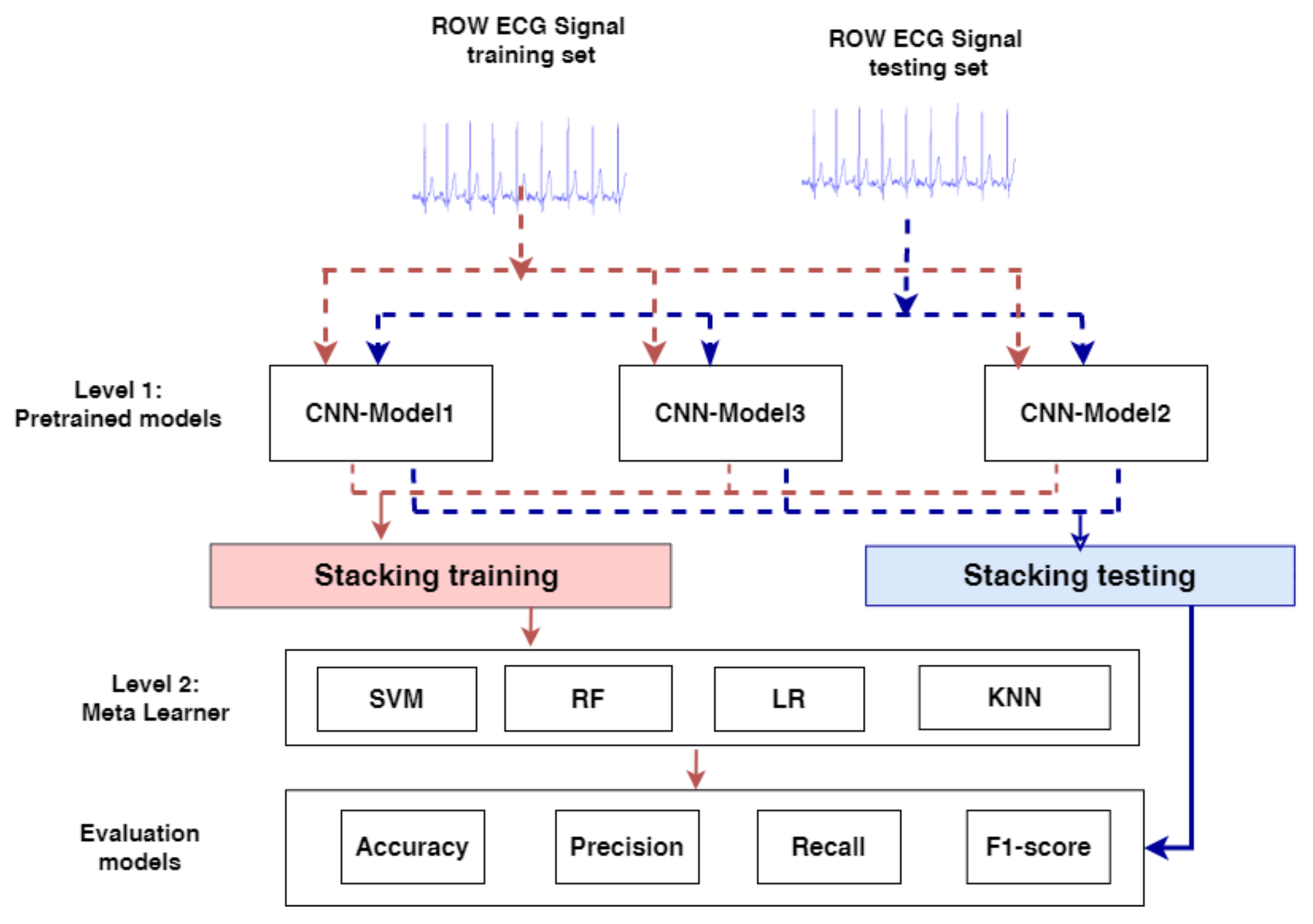
3.3. The Proposed Model

The proposed model is comprised of a stacking ensemble that consists of two primary levels, Level-1 and Level-2, as seen in Figure 2.

• In Level-1, First, the pre-trained CNN models, CNN-Model1, CNN-Model2, and CNN-Model3, are loaded; excluding the output layer, all the model layers are frozen. Because the pretrained models will not be trained again and their parameters have been frozen, they will have no effect on the fine ensemble model’s complexity. Second, in stacking training, the output probabilities of each CNN model’s training set are merged, so in the stacking test, the output probabilities of each CNN model’s testing set are combined;
• In Level-2, stacking training is used to train and optimize the meta-learners: SVM [49,50], LR, KNN, and RF and stacking testing are used to evaluate the meta-learners and make the final prediction results. We optimized the meta-learners by using grid search and some of the parameters are also adapted for each model.

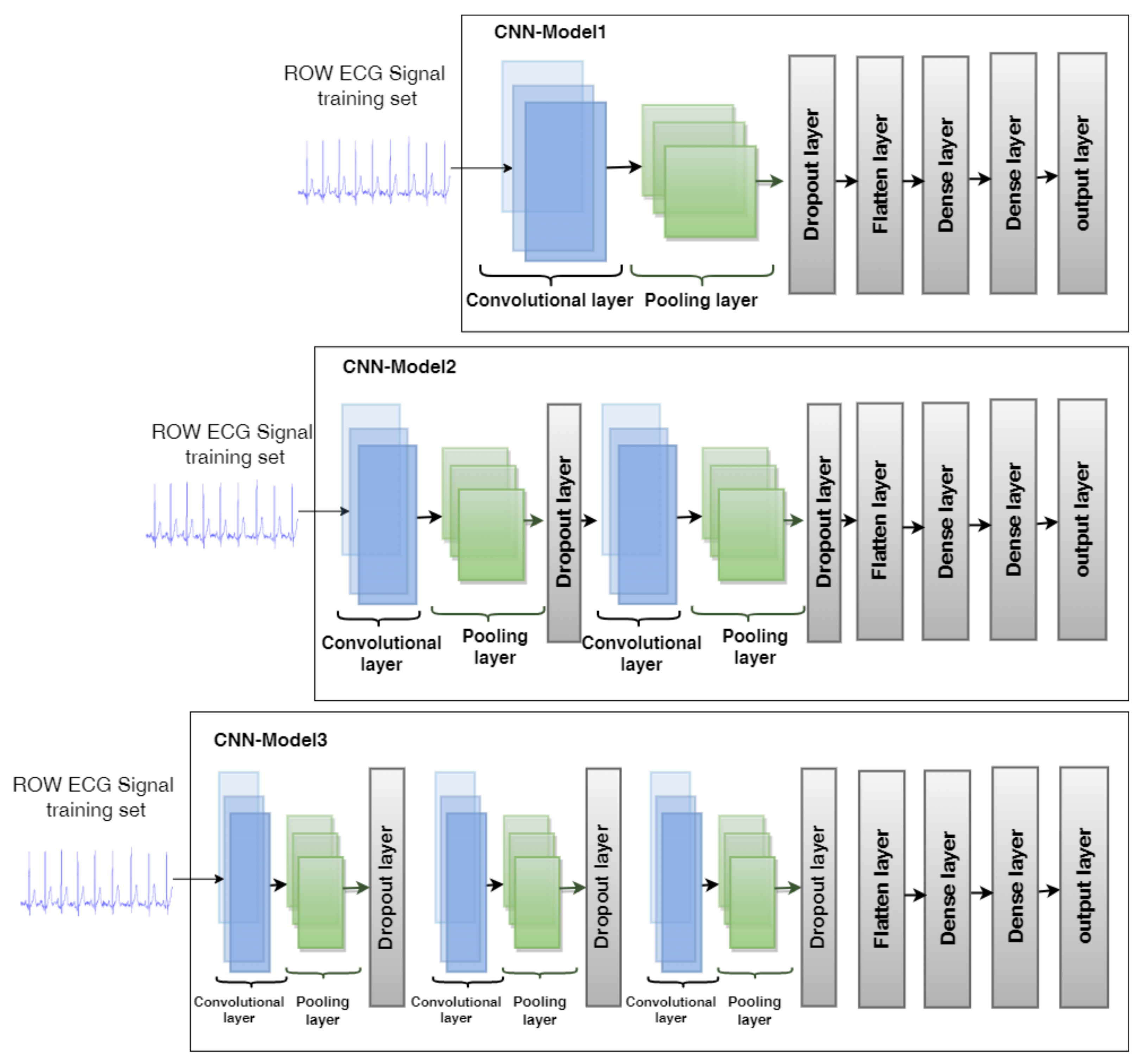
3.3.1. CNN Model Architectures

The training of CNNs enables the automated extraction of high-level features. In this study, three CNN models: CNN-Model1, CNN-Model2, and CNN-Model3, are proposed for the classification of heartbeats. The structure of the three CNN models is illustrated in Figure 3.

• CNN-Model1 is made up of a convolutional layer, a Max-pooling layer, a dropout layer, a flatten layer, a dense layer, a fully connected layer, and an output layer;
• CNN-Model2 comes with two convolutional layers, two max-pooling layers, two dropout layers, flatten layer, dense layer, fully connected layer, and output layer;
• CNN-Model3 is comprised of three convolutional layers, three max-pooling layers, three dropout layers, a flatten layer, a dense layer followed by a fully connected layer, and an output layer.
  We will discuss each layer of CNN models in the following detail.

  -

  The convolutional layer is the first layer utilized to extract the various features, which also carries the bulk of the computation [51]. The convolution process is carried out in this layer between the input and a window filter by swiping the filter over the input to calculate the dot product between the filter and the input’s parts while accounting for the filter’s size [52,53]. The feature map, which represents the output, provides details about the input. When the convolution layer has finished applying the convolution operation to the input, it transfers the results to the subsequent layer. ReLU activation function is also employed, which reduces the possibility that the computation required to operate the neural network would increase exponentially [54]. As the size of the CNN scales, the computational cost of adding more ReLUs increases linearly;

  -

  The pooling layer’s goal is to reduce the size of the convoluted feature map to lower the computational expenses by scaling down the representation’s spatial scope and minimizing the necessary computations [55]. The features created by a convolution layer are enumerated here. Max pooling uses a feature map to determine its largest component [56];

  -

  The flattening layer is used to transform the data in the pooling layer into feature vectors;

  -

  Fully connected layers are employed to connect the neurons between two separate layers. The neurons, as well as the weights and biases, are included in these layers. These layers are often positioned before the output layer and make up the final few layers of a CNN architecture [57]. The last layers’ flattened input is sent to the fully connected layer [58];

  -

  A dropout layer eliminates a few neurons from the neural network during training to both minimize the size of the model and solve the overfitting issue [59];

  -

  The output layer is the final layer of models that are used to make the final decisions; when we used the MIT-BIH dataset, the output layer had five neurons equivalent to the classes considered: Normal (N), Article Premature(AP), Premature ventricular contraction(PVC), Fusion of ventricular and normal (FVN), and Fusion of paced and normal (FPN), and softmax [60] was used as an activation function. When we used the PTB, the output layer has two neurons that are equivalent to the considered classes: normal and abnormal. Additionally, sigmoid [61] is used as the activation function.

3.3.2. Optimization Methods for CNN Models

The Keras Tuner is a framework that assists in the selection of the best set of hyperparameters for a model that is based on the Bayesian optimizer. Hyperparameters are the factors that influence the training process as well as the structure of a CNN model. These variables are present throughout the training process, having a direct influence on the model’s performance [62]. For optimized CNN models, we adapted some of the values of hyperparameters for CNN-Model1, CNN-Model2, and CNN-Model3 for each dataset, as shown in

Table 2. The hyperparameter values of the CNN models.

Parameters	CNN-Model1	CNN-Model2	CNN-Model3
Filter_Size	[16,128,256]	[16,128,256]	[16,128,256]
Kernel_size	[4,5]	[4,5]	[4,5]
Pool_Size	[2,3]	[2,3]	[2,3]
Dense1_Unit	20 to 500 step 20	20 to 500 step 20	20 to 500 step 20
Dense2_Unit	20 to 400 step 20	20 to 400 step 20	20 to 400 step 20

.

3.3.3. Optimization Methods for Meta-Learner Classifiers

The stacked output probabilities of the CNN models for the training set were trained and optimized using the meta-learner classifiers LR, SVM, KNN, and RF. Grid search has been used to optimize the meta-learner classifiers., and we adapted some of the values of hyperparameters for each meta-learner classifier as follows. SVM: C = [0.1, 1, 10, 100, 1000], gamma = [1, 0.1, 0.01, 0.001, 0.0001], kernel = RBF; KNN: K = [10,20,30,40]; RF: bootstrap = [True, False], max_depth = [10, 20, 30, 40, 50, 60], max_features = [’auto’, ’sqrt’], min_samples_leaf = [2, 5, 10], min_samples_split = [1, 2, 4], LR: C= np.logspace (−3, 3, 7) penalty = [“l2”], solver = [’liblinear’, ’newton-cg’].

3.4. Evaluation

The classification performances were measured by using the following four metrics: accuracy (ACC), precision (PRE), recall (REC), and F1-score (F1).

• Accuracy can be expressed as a measure of how many real positives and real negatives there are compared to all the positive and negative observations. The performance statistics for the classification models are created using machine learning. In other words, accuracy represents the percentage of the model’s predictions, effectively predicting a given outcome [63].

  $$\mathrm{Accuracy}=\frac{\mathrm{TP}+\mathrm{TN}}{\mathrm{TP}+\mathrm{FP}+\mathrm{TN}+\mathrm{FN}}.$$

  (1)
• Precision represents the proportion of labels that are correctly predicted to be positive. It is commonly known as the “positive predictive value,” which is affected by the class distribution [63].

  $$\mathrm{Precision}=\frac{\mathrm{TP}}{\mathrm{TP}+\mathrm{FP}}$$

  (2)
• Recall measures how well a model can predict positive outcomes from actual positive outcomes, unlike precision, which measures the percentage of correct positive predictions across all positive predictions made by models [63].

  $$\mathrm{Recall}=\frac{\mathrm{TP}}{\mathrm{TP}+\mathrm{FN}}$$

  (3)
• F-score is an ML model performance measure that determines how accurate a model is, and it equally weights Precision and Recall [63].

  $$\mathrm{F}1-\mathrm{score}=\frac{2·\mathrm{precision}·\mathrm{recall}}{\mathrm{precision}+\mathrm{recall}}$$

  (4)

The number of correctly created positively predicted values is denoted by TP, the number of wrongly made negatively predicted values by FP, the number of correctly made positively predicted negative values by TN, and the number of correctly made positively predicted phrases by FN.

4. Experimental Results

In this section, we describe the results of performing the models, which are categorized into ML models (DT, KNN, RF, and SVM), CNN model (CNN-Model-1, CNN-Model-2, CNN-Model-3), and our proposed ensemble model, which is ensemble stacking based on four meta-learner classifiers SVM, RF, LR, and KNN for two datasets: MIT-BIH, and PTB.

4.1. Experimental Setup

The experiments in this work are conducted on Google Colab with GPU. The Scikit-learn library is used to implement ML models, and the Keras library is used to implement CNN models.

Each dataset is split by an 80% training set and a 20% testing.

4.2. Results of the MIT-BIH Dataset

This section presents the PRE, REC, and F1 results for each class and shows the average of ACC, PRE, REC, and F1 for ML, CNN models, and the proposed model-based meta-learner classifiers for the MIT-BIH dataset. In the CNN models, we adapted some parameters: a batch_size of 1000, epoch = 20, and learning rate = 0.00004, the optimizer Adam Keras Tuner was used to optimize the CNN models, and the final values of each parameter of CNN-Model1, CNN-Model2, and CNN-Model3 were applied to the MIT-BIH dataset, as shown in

Table 3. Values of the parameters after applying the CNN models to the MIT-BIH dataset.

Datasets	Models	Filter Size	Kernel Size	Pooling Size	Dropout Values	#Units of Dense1	#Units of Dense2
MIT-BIH dataset	CNN-Model1	16	5	2	0.5	20	40
	CNN-Model2	[256,256]	[5,4]	[2,2]	[0.2,0.2]	440	240
	CNN-Model3	[256,256,128]	[4,5,5]	[2,2,2]	[0.5,0.6,0.6]	240	340

. Second, the stacked output probabilities of CNN models were trained and optimized using the meta-learner classifiers LR, SVM, KNN, and RF. Grid search has been used to optimize the meta-learner classifiers, and the best values of hyperparameters for each meta-learner classifier were as follows. SVM: C = 10, gamma = 1, kernel = RBF; KNN, K = 20, RF: bootstrap = True, max_depth = 70, max_features = auto, min_samples_leaf = 2, min_samples_split = 5, LR: C = 100, penalty = l2, solver = liblinear.

4.2.1. The Results of Each Class

Table 4. The average ACC, PRC, REC, and F1 when applying the models to the MIT-BIH dataset.

Approaches	Models	Evaluation Metrics	Testing Performance
			N	AP	PVC	FVN	FPN
ML approach	DT	PRE	98	64	97	60	94
		REC	98	65	86	61	94
		F1	98	64	91	60	94
	RF	PRE	97	98	98	78	99
		REC	98	69	88	65	96
		F1	98	76	93	71	98
	SVM	PRE	97	96	97	75	100
		REC	100	56	86	48	91
		F1	98	71	91	59	95
	KNN	PRE	98	90	94	76	99
		REC	99	66	90	64	95
		F1	99	75	92	69	97
CNN approach	CNN-Model1	PRE	97	93	93	80	99
		REC	99	60	89	49	92
		F1	98	73	91	61	96
	CNN-Model2	PRE	99	90	95	87	100
		REC	100	77	94	72	98
		F1	99	83	95	79	99
	CNN-Model3	PRE	96	92	95	78	98
		REC	99	52	79	43	95
		F1	98	67	86	55	96
The proposed model	SVM meta classifier	PRE	99	94	97	84	99
		REC	100	97	95	80	99
		F1	99	86	96	82	99
	RF meta classifier	PRE	99	98	99	89	100
		REC	100	98	98	85	99
		F1	99	89	99	87	100
	LR meta classifier	PRE	99	98	97	82	99
		REC	100	79	95	75	99
		F1	99	86	96	79	99
	KNN meta classifier	PRE	99	91	97	85	99
		REC	100	80	95	78	99
		F1	99	85	96	80	99

shows the PRE, REC, and F1 results for each class in the MIT-BIH dataset.

• ML models results
  For the N class, SVM registers the highest REC at 100. DT and, KNN, RF register the same PRE at 98. For the AP class, RF registers the highest PRE, REC, and F1 at 98, 69, and 76, respectively. KNN has the second-highest F1 at 75. DT records the lowest PRE, REC, and F1 at 64, 65, and 64, respectively. For the PVC class, RF registers the highest PRE, REC, and F1 at 98, 88, and 93, respectively. KNN registers the second highest REC and F1 at 90 and 92, respectively. DT and SVM record the second-highest PRE at 97. For the FVN class, RF registers the highest PER, REC, and F1 at 88, 65, and 71, respectively. SVM notes the lowest REC and F1 at 48 and 95, respectively. For the FPN class, SVM registers the highest PRE at 100. RF has the highest REC and F1 at 96 and 98, respectively. DT records the lowest PRE and F1 at 94;
• CNN models results
  For the N class, CNN-Model2 registers the highest REC, REC, and F1 at 99, 100, and 99, respectively. CNN-Model1 and CNN-Model3 register the same PRE at 98. CNN-Model3 has the lowest PRE at 96. For the AP class, CNN-Model1 registers the highest PRE at 93. CNN-Model2 records the highest REC and F1 at 77 and 83, respectively. CNN-Model3 has the lowest REC and F1 at 52 and 67, respectively. For the PVC class, CNN-Model2 registers the highest REC, REC, and F1 at 95, 94, and 95, respectively. CNN-Model3 has the lowest REC and F1 at 97 and 86, respectively. For the FVN class, CNN-Model2 registers the highest PER, REC, and F1 at 87, 72, and 79, respectively. CNN-Model3 reports the lowest REC and F1 at 43 and 55, respectively. For the FPN class, CNN-Model2 registers the highest PRE, REC, and F1 at 100, 98 and 99, respectively. CNN-Model1 records the lowest REC at 92.
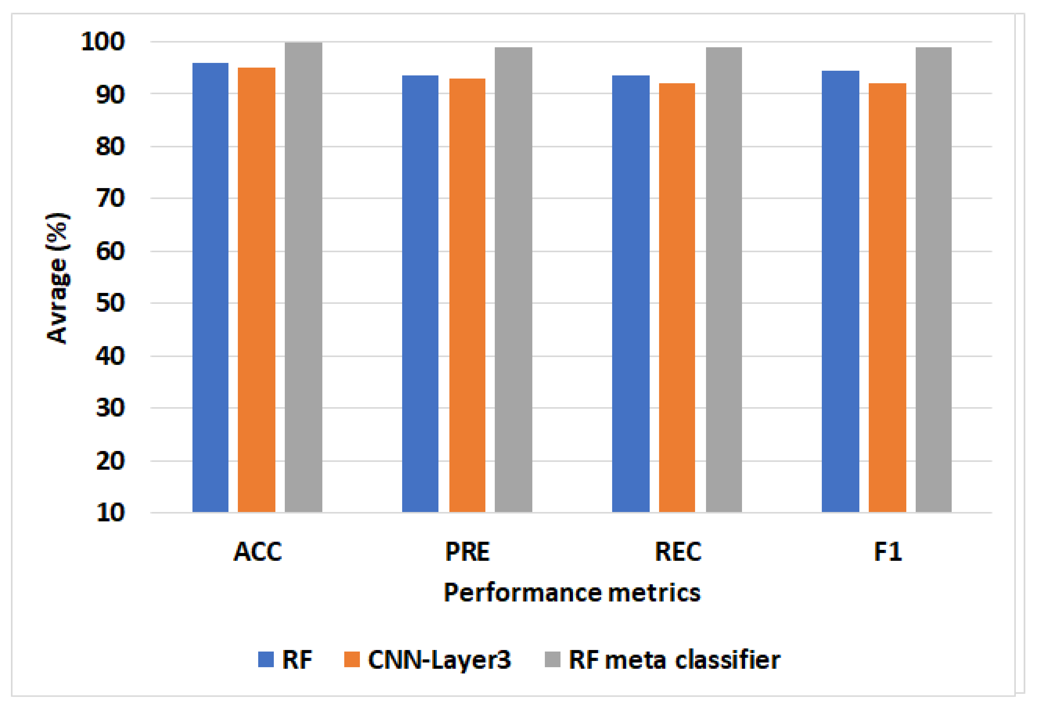
• In the proposed model, we used different meta-leaner models (SVM, RF, LR, and KNN). For N class, all meta classifiers have the same PRE, REC, and F1 scores at 99, 100, and 99, respectively. For the AP class, the RF meta classifier records the highest PRE, REC, and F1 scores at 98, 98, and 89, respectively. The KNN meta classifier records the lowest PRE, REC, and F1 scores at 91, 80, and 85, respectively. For the PVC class, stacking RF records the highest PRE, REC, and F1 scores at 99, 98, and 99, respectively. KNN, LR, and SVM meta classifiers record the same scores of PRE, REC, and F1 scores at 97, 95, and 96, respectively. For the FVN class, the RF meta classifier records the highest PRE, REC, and F1 scores at 89, 85, and 87, respectively. The LR meta classifier records the lowest scores of PRE, REC, and F1 scores at 82, 75, and 79, respectively. For the FVN class, the RF meta classifier records the highest PRE and F1 scores at 100. SVM, LR, and KNN SVM meta classifiers record the same scores of PRE, REC, and F1 at 99.

4.2.2. The Average of the Performance Methods

Table 5. The average of ACC, PRC, REC, and F1 when applying the models to the MIT-BIH dataset.

Models	ACC	PRE	REC	F1
DT	95	82.6	80.8	81
SVM	96	93	76.2	82.8
KNN	97	91.4	82.4	86.4
RF	95	94	83.2	87.2
CNN-Layer1	97	92.4	77.8	83.8
CNN-Layer2	98	94.2	88.2	91
CNN-Layer3	96	91.8	73.6	80.4
SVM meta classifier	98	94.6	94.2	92.4
RF meta classifier	99.8	97	96	94.8
LR meta classifier	98	95	89.6	91.8
KNN meta classifier	98	94.2	90.4	91.8

represents the average ACC, PRC, REC, and F1 of applying models to the MIT-BIH dataset. We can see that the proposed model records the highest performance compared to other models, ML, and CNN. The proposed model-based RF meta-classifier achieves the highest average of ACC, PRC, REC, and F1 at 99.8, 97, 96, and 94.8, respectively, compared to other models. The SVM meta classifier achieves the second-highest average of ACC, PRC, REC, and F1 at 98, 94.6, 94.2, and 92.4, respectively. In the ML models, RF records the highest average of ACC, PRC, REC, and F1 at 95, 94, 83.2, and 87.2, respectively. DT records the lowest average of ACC, PRC, and F1 at 95, 82.6, and 81, respectively. In CNN models, CNN-Layer2 records the highest average of ACC at 98, 94.2, 88.2, and 91, respectively.

4.3. Results of the PTB Dataset

This section presents the PRE, REC, and F1 results for each class and shows the average of ACC, PRE, REC, and F1 for ML, CNN models, and the proposed model-based meta-learner classifiers for the PTB dataset.

First, in the CNN models, we adapted some parameters: batch_size of 500 and epoch = 20, learning rate = 0.00004, and Adam as the optimizer. Keras Tuner was used to optimize the CNN models, and the final values of each parameter of CNN-Model1, CNN-Model2, and CNN-Model3 were the PTB datasets, as shown in

Table 6. The values of the parameters after applying the CNN models to the MIT-BIH and PTB dataset.

Datasets	Models	Filter Size	Kernel Size	Pooling Size	Dropout Values	#Units of Dense1	#Units of Dense2
PTB dataset	CNN-Model1	16	4	2	0.8	460	300
	CNN-Model2	[256,128]	[4,5]	[2,2]	[0.8,0.7]	480	200
	CNN-Model3	[128,256,256]	[5,4,5]	[2,2,2]	[0.6,0.5,0.4]	300	220

.

Second, the stacked output probabilities of the CNN models were trained and optimized using the meta-learner classifiers LR, SVM, KNN, and RF. Grid search was used to optimize the meta-learner classifiers, and the best values of the hyperparameters for each meta-learner classifier were as follows. SVM: C = 100, gamma = 1, kernel = RBF; KNN, K = 9, RF: bootstrap = True, max_depth = 50, max_features = auto, min_samples_leaf = 5, min_samples_split = 5, LR: C = 10, penalty=l2, solver = liblinear.

4.3.1. The Results of Each Class

Table 7. The PRE, REC, and F1 results for each class in the PTB dataset.

Approaches	Models	Evaluation Metrics	Normal	Abnormal
ML approach	DT	PRE	86	94
		REC	88	95
		F1	87	95
	SVM	PRE	86	93
		REC	81	95
		F1	83	94
	KNN	PRE	86	96
		REC	91	94
		F1	88	95
	RF	PRE	90	97
		REC	89	98
		F1	92	97
DL approach	CNN-Layer1	PRE	94	94
		REC	82	96
		F1	88	98
	CNN-Layer2	PRE	85	94
		REC	86	95
		F1	86	95
	CNN-Layer3	PRE	92	94
		REC	91	93
		F1	91	93
The proposed models	SVM meta classifier	PRE	98	99
		REC	98	99
		F1	98	99
	RF meta classifier	PRE	99	99
		REC	99	99
		F1	99	99
	LR meta classifier	PRE	98	99
		REC	98	99
		F1	98	99
	KNN meta classifier	PRE	97	99
		REC	97	99
		F1	97	99

shows PRE, REC, and F1 results for each class in the PTB dataset

• ML models results
  For the normal class, RF registers the highest PRE, REC, and F1 at 90, 89, and 92, respectively. KNN reports the second-highest REC at 91 and F1 at 88. DT, SVM, and KNN register the same PRE at 86. SVM records the lowest F1 at 83. For the abnormal class, RF registers the highest PRE, REC, and F1 at 97, 98, and 97, respectively KNN registers the highest REC at 96 and F1 at 95. DT and SVM register the same PRE at 95. SVM records the lowest PRE at 93;
• CNN models results
  For the normal class, CNN-Model1 registers the highest PRE at 94 and records the lowest REC at 82. CNN-Model3 records the highest REC and F1 at 91. For the abnormal class, CNN-Model1 registers the highest PRE, REC, and F1 at 94, 96, and 98, respectively. CNN-Model2 reports the second high of REC and F1 at 95;
• Our proposed model result
  For normal class, the RF meta classifier registers the highest PRE, REC, and F1 at 99. SVM and LR meta classifiers register the second highest PRE, REC, and F1 at 98. KNN writes the lowest PRE, REC, and F1 at 99. For the abnormal class, RF, LR, SVM, and KNN register the same PRE, REC, and F1 at 99.

4.3.2. The Average of the Performance Methods

Table 8. The average ACC, PRC, REC, and F1 when applying the models to the PTB dataset.

Approaches	Models	ACC	PRC	REC	F1
ML approach	DT	93	90	91.5	91
	SVM	91	89.5	88	88.5
	KNN	93	91	92.5	91.5
	RF	96	93.5	93.5	94.5
CNN approach	CNN-Layer1	94	92	89	93
	CNN-Layer2	92	89.5	90.5	90.5
	CNN-Layer3	95	93	92	92
The proposed models	SVM meta classifier	98	98.5	98.5	98.5
	RF meta classifier	99.7	99	99	99
	LR meta classifier	98	98.5	98.5	98.5
	KNN meta classifier	98	98	98	98

represents the average ACC, PRC, REC, and F1 when applying the models to the PTB dataset. We can see that the proposed model records the highest performance compared to other models, ML, and CNN models. The proposed model-based RF meta-classifier achieves the highest average of ACC, PRC, REC, and F1 at 99.7, 99, 99, and 99, respectively, compared to other models. LR meta classifier achieves the second-highest average of ACC, PRC, REC, and F1 at 98, 98.5, 98.5, and 98.5, respectively. In ML models, RF records the highest average of ACC, PRC, REC, and F1 at 96, 93.5, 93.5, and 94.5, respectively. KNN records the lowest average of ACC, PRC, REC, and F1 at 91, 89.5, 88, and 88.5, respectively. In CNN models, CNN-Layer3 records the highest average of ACC at 95, 93, 92, and 92, respectively.

4.4. Discussion

We discuss three ML models (DT, KNN, and SVM), three CNN models, and our proposed model using datasets for MIT-BIH, and PTB datasets for MI. In this section, a discussion of the summarized experimental results is introduced.

MIT-BIH

Figure 4 represents the best ML, CNN, and proposed models for the MIT-BIH dataset. We can see that the proposed model-based RF meta classifier achieves the best performance compared to RF and CNN-Model2. The RF meta classifier improves ACC by 4.8, PRC by 3, REC by 7.6, and F1 by 4 compared to RF. The RF meta classifier improves ACC by 1.8, PRC by 2.8, REC by 5.5, and F1 by 4.5, compared to the CNN-Layer3.

4.5. PTB Dataset

Figure 5 represents the best ML, CNN, and proposed models for the PTB dataset. We can see that the proposed model-based RF meta classifier achieves the best performance compared to RF and CNN-Model3. The RF meta classifier improves ACC by 4, PRC by 5.5, REC by 5.5, and F1 by 4.5 compared to RF. The RF meta classifier improves ACC by 5, PRC by 6, REC by 7, and F1 by 7 compared to CNN-Layer3.

Comparison with Literature Studies

We compared the proposed model with the previous studies that have used the MIT-BIH and PTB datasets, see

Table 9. Comparison of the performance of the proposed model with the previous studies.

Papers	Models	Datasets	Performance
[22]	12-layer deep of 1D CNN	MIT-BIH	ACC = 97.41
[23]	7-layer deep of 1D CNN	MIT-BIH	ACC = 98.74
[30]	CNN-GRU	MIT-BIH	ACC = 99.61 F1 = 99.42
[31]	combining LSTM and CNN	MIT-BIH	ACC = 99
[32]	combined CNN and RNN	MIT-BIH	ACC = 95.90
[33]	combined CNN and SVM	MIT-BIH	ACC = 91.29
[24]	CNN	MIT-BIH	ACC = 93.6
[25]	CNN	MIT-BIH	ACC = 97.5
[26]	CNN	PTB	ACC = 98.84 PRC = 98.31, REC = 97.92 F1 = 97.63
[35]	3 layers of LSTM	PTB	PRE = 91 F1 = 90
[36]	ANN	PTB	ACC = 90.1
[27]	CNN	PTB	ACC = 99
[37]	LS-SVM	PTB	ACC = 99.31
[28]	CNN	PTB	ACC = 95.22
[34]	CNN-LSTM	PTB	F1 = 94.6
The proposed model	RF meta-learner classifier	MIT-BIH	ACC = 99.8 PRE = 97 REC = 96 F1 = 94.8
The proposed model	RF meta-learner classifier	PTB	ACC = 99.7 PRE = 99 REC = 99 F1 = 99

. For the MIT-BIH dataset, ACC of a 12-layer deep model of 1D CNN in Ref. [22] was recorded at 97.41%. In Ref. [23], the ACC of a 7-layer deep model of 1D CNN was recorded as 98.74%. In Refs. [23,24], ACC of CNN was registered as 93.6% and 97.5%, respectively. Other authors used hybrid models. For example, in Ref. [30], ACC of CNN-GRU was recorded at 99.61%, and F1 was recorded at 99.42%. In Ref. [31], ACC of combining an LSTM model and CNN model was recorded at 99%. In Ref. [32], ACC of combined CNN and RNN was recorded at 95.9%. In Ref. [32], ACC of combined CNN and SVM was recorded at 95.9%. The proposed model-based RF meta-classifier achieved the highest average for ACC, PRC, REC, and F1 with 99%, 97%, 96%, and 94.8%, respectively.

For the PTB dataset, ACC, PRC, REC, and F1 of CNN were recorded as 98.84%, 98.31%, 97.92%, and 97.63%, respectively, in Ref. [26]. In Ref. [35], 3-layers of LSTM were recorded with PRC of 91% and F1 90%. In Ref. [36], ACC of an ANN model was obtained at 91.1%. In RefS. [27,28], the ACC of a CNN model was recorded at 99% and 95.2%, respectively. In Ref. [37], LS-SVM was recorded at 99.31%. In Ref. [34], F1 of CNN-LSTM was recorded at 94.6%. The proposed model-based RF meta-classifier achieved the highest average of ACC, PRC, REC, and F1 at 99.7%, 99%, 99%, and 99%, respectively.

5. Limitations and Future Directions

The proposed deep learning ensemble model has advanced the literature on deep learning in the medical domain. We used the Bayesian optimizer to select the best stacking deep ensemble model. Several experiments have been explored to choose the best architectures for base classifiers and for selecting the meta-learner. The resulting model achieved the best results compared to the literature by using two different datasets. However, the proposed model still has some limitations that will be handled in future studies. For example, the model will be tested using other data sets to check its stability. The proposed ensemble is more complex than each of the base models. The complexity of the resulting stacking ensemble will be explored to make a trade-off between the time complexity and the gained results. The resulting model is a black box, and medical experts should not trust the model results. We will explore the possible ways to improve the model transparency in a future study.

6. Conclusions

In this paper, a stacking ensemble model based on CNN was proposed in order to identify the patients at risk of MI. The proposed model incorporated two main primary levels; In Level-1, first, the pre-trained CNN models: CNN-Model1, CNN-Model2, and CNN-Model3 are loaded; excluding the output layer, all layers of the models were frozen. Second, in stacking training, the output probabilities of each CNN model’s training set were merged, so in stacking testing, the output probabilities of each CNN model’s testing set are combined. In Level-2, stacking training was used to train and optimize the meta-learners: SVM, LR, KNN, RF, and stacking testing were used to evaluate the meta-learners and make the final prediction results. We optimized the meta-learners using grid search, and some of the parameters were adapted for each model. The experimental results have significantly demonstrated our proposed model’s superiority over the other models for the three datasets. For the MIT-BIH dataset, the proposed model based on the RF meta-learner classifier obtained the highest score for ACC with 99.8%,, PRE with 97%, REC with 96%,, and F1 with 94.8%,, outperforming all the other methods. For the PTB dataset, the proposed model based on the RF meta-learner classifier has the highest scores of ACC with 99.7%, PRE with 99%, REC with 99%, and F1 with 99%, exceeding all the other methods.

References

- Centers for Disease Control and Prevention. National Center for Health Statistics Mortality Data on CDC WONDER. Available online: https://wonder.cdc.gov/mcd.html (accessed on 10 October 2022).
- Tsao, C.W.; Aday, A.W.; Almarzooq, Z.I.; Alonso, A.; Beaton, A.Z.; Bittencourt, M.S.; Boehme, A.K.; Buxton, A.E.; Carson, A.P.; Commodore-Mensah, Y.; et al. Heart disease and stroke statistics—2022 update: A report from the American Heart Association. Circulation 2022, 145, e153–e639. [Google Scholar]
- Singh, A.; Gupta, A.; Collins, B.L.; Qamar, A.; Monda, K.L.; Biery, D.; Lopez, J.A.G.; de Ferranti, S.D.; Plutzky, J.; Cannon, C.P.; et al. Familial hypercholesterolemia among young adults with myocardial infarction. J. Am. Coll. Cardiol. 2019, 73, 2439–2450. [Google Scholar]
- Singh, A.; Collins, B.L.; Gupta, A.; Fatima, A.; Qamar, A.; Biery, D.; Baez, J.; Cawley, M.; Klein, J.; Hainer, J.; et al. Cardiovascular risk and statin eligibility of young adults after an MI: Partners YOUNG-MI Registry. J. Am. Coll. Cardiol. 2018, 71, 292–302. [Google Scholar] [CrossRef]
- Tregilgas, R.B. Diagnosis and treatment of myocardial infarction. J. Lancet 1959, 79, 538–544. [Google Scholar]
- Richardson, W.; Clarke, S.; Alexander Quinn, T.; Holmes, J. Physiological implications of myocardial scar structure. Compr. Physiol. 2015, 5, 1877. [Google Scholar]
- Kong, Q.; Wu, Y.; Yuan, C.; Wang, Y. CT-CAD: Context-Aware Transformers for End-to-End Chest Abnormality Detection on X-Rays. In Proceedings of the 2021 IEEE International Conference on Bioinformatics and Biomedicine (BIBM), Houston, TX, USA, 9–12 December 2021; pp. 1385–1388. [Google Scholar]
- Wu, Y.; Yue, Y.; Tan, X.; Wang, W.; Lu, T. End-to-end chromosome Karyotyping with data augmentation using GAN. In Proceedings of the 2018 25th IEEE International Conference on Image Processing (ICIP), Athens, Greece, 7–10 October 2018; pp. 2456–2460. [Google Scholar]
- Wu, Y.; Zhang, L.; Berretti, S.; Wan, S. Medical Image Encryption by Content-aware DNA Computing for Secure Healthcare. IEEE Trans. Ind. Inform. 2022, in press. [Google Scholar] [CrossRef]
- Chen, J.; Chen, W.; Zeb, A.; Zhang, D. Segmentation of medical images using an attention embedded lightweight network. Eng. Appl. Artif. Intell. 2022, 116, 105416. [Google Scholar] [CrossRef]
- Saleh, H.; Mostafa, S.; Gabralla, L.A.; Aseeri, O.A.; El-Sappagh, S. Enhanced Arabic Sentiment Analysis Using a Novel Stacking Ensemble of Hybrid and Deep Learning Models. Appl. Sci. 2022, 12, 8967. [Google Scholar] [CrossRef]
- Saleh, H.; Alharbi, A.; Alsamhi, S.H. OPCNN-FAKE: Optimized convolutional neural network for fake news detection. IEEE Access 2021, 9, 129471–129489. [Google Scholar] [CrossRef]
- Hammam, A.A.; Elmousalami, H.H.; Hassanien, A.E. Stacking deep learning for early COVID-19 vision diagnosis. In Big Data Analytics and Artificial Intelligence Against COVID-19: Innovation Vision and Approach; Springer: Berlin/Heidelberg, Germany, 2020; pp. 297–307. [Google Scholar]
- Cao, D.; Xing, H.; Wong, M.S.; Kwan, M.P.; Xing, H.; Meng, Y. A stacking ensemble deep learning model for building extraction from remote sensing images. Remote. Sens. 2021, 13, 3898. [Google Scholar] [CrossRef]
- Brownlee, J. Ensemble learning methods for deep learning neural networks. 2018. Available online: https://machinelearningmastery.com/ensemble-methods-for-deep-learning-neural-networks/ (accessed on 10 October 2022).
- Nanehkaran, Y.A.; Chen, J.; Salimi, S.; Zhang, D. A pragmatic convolutional bagging ensemble learning for recognition of Farsi handwritten digits. J. Supercomput. 2021, 77, 13474–13493. [Google Scholar] [CrossRef]
- Wang, J.; Feng, K.; Wu, J. SVM-based deep stacking networks. In Proceedings of the AAAI Conference on Artificial Intelligence, Atlanta, GE, USA, 8–12 October 2019; Volume 33, pp. 5273–5280. [Google Scholar]
- Ganaie, M.A.; Hu, M.; Malik, A.K.; Tanveer, M.; Suganthan, P.M. Ensemble deep learning: A review. arXiv 2014, arXiv:2104.02395. [Google Scholar]
- Jin, L.; Dong, J. Ensemble deep learning for biomedical time series classification. Comput. Intell. Neurosci. 2016, 2016, 6212684. [Google Scholar] [CrossRef]
- Chen, J.; Zeb, A.; Nanehkaran, Y.; Zhang, D. Stacking ensemble model of deep learning for plant disease recognition. J. Ambient. Intell. Humaniz. Comput. 2022, 1–14. Available online: https://link.springer.com/article/10.1007/s12652-022-04334-6 (accessed on 10 October 2022).
- Zhang, B.; Qi, S.; Monkam, P.; Li, C.; Yang, F.; Yao, Y.D.; Qian, W. Ensemble learners of multiple deep CNNs for pulmonary nodules classification using CT images. IEEE Access 2019, 7, 110358–110371. [Google Scholar] [CrossRef]
- Wu, M.; Lu, Y.; Yang, W.; Wong, S.Y. A study on arrhythmia via ECG signal classification using the convolutional neural network. Front. Comput. Neurosci. 2021, 14, 564015. [Google Scholar] [CrossRef]
- Zhang, Y.; Liu, S.; He, Z.; Zhang, Y.; Wang, C. A CNN Model for Cardiac Arrhythmias Classification Based on Individual ECG Signals. Cardiovasc. Eng. Technol. 2022, 13, 548–557. [Google Scholar] [CrossRef] [PubMed]
- Rajkumar, A.; Ganesan, M.; Lavanya, R. Arrhythmia classification on ECG using Deep Learning. In Proceedings of the 2019 5th International Conference on Advanced Computing & Communication Systems (ICACCS), Coimbatore, India, 15–16 March 2019; pp. 365–369. [Google Scholar]
- Li, D.; Zhang, J.; Zhang, Q.; Wei, X. Classification of ECG signals based on 1D convolution neural network. In Proceedings of the 2017 IEEE 19th International Conference on e-Health Networking, Applications and Services (Healthcom), Dalian, China, 12–15 October 2017; pp. 1–6. [Google Scholar]
- Hammad, M.; Alkinani, M.H.; Gupta, B.; El-Latif, A.; Ahmed, A. Myocardial infarction detection based on deep neural network on imbalanced data. Multimed. Syst. 2022, 28, 1373–1385. [Google Scholar] [CrossRef]
- Baloglu, U.B.; Talo, M.; Yildirim, O.; San Tan, R.; Acharya, U.R. Classification of myocardial infarction with multi-lead ECG signals and deep CNN. Pattern Recognit. Lett. 2019, 122, 23–30. [Google Scholar] [CrossRef]
- Acharya, U.R.; Fujita, H.; Oh, S.L.; Hagiwara, Y.; Tan, J.H.; Adam, M. Application of deep convolutional neural network for automated detection of myocardial infarction using ECG signals. Inf. Sci. 2017, 415, 190–198. [Google Scholar] [CrossRef]
- Cheng, J.; Zou, Q.; Zhao, Y. ECG signal classification based on deep CNN and BiLSTM. BMC Med. Inform. Decis. Mak. 2021, 21, 1–12. [Google Scholar] [CrossRef]
- Yao, G.; Mao, X.; Li, N.; Xu, H.; Xu, X.; Jiao, Y.; Ni, J. Interpretation of electrocardiogram heartbeat by CNN and GRU. Comput. Math. Methods Med. 2021, 2021, 6534942. [Google Scholar] [CrossRef] [PubMed]
- Zhang, P.; Cheng, J.; Zhao, Y. Classification of ECG Signals Based on LSTM and CNN. International Conference on Artificial Intelligence and Security; Springer: Berlin/Heidelberg, Germany, 2020; pp. 278–289. [Google Scholar]
- Xu, X.; Jeong, S.; Li, J. Interpretation of electrocardiogram (ECG) rhythm by combined CNN and BiLSTM. IEEE Access 2020, 8, 125380–125388. [Google Scholar] [CrossRef]
- Liu, J.; Song, S.; Sun, G.; Fu, Y. Classification of ECG arrhythmia using CNN, SVM and LDA. In International Conference on Artificial Intelligence and Security; Springer: Berlin/Heidelberg, Germany, 2019; pp. 191–201. [Google Scholar]
- Lui, H.W.; Chow, K.L. Multiclass classification of myocardial infarction with convolutional and recurrent neural networks for portable ECG devices. Inform. Med. Unlocked 2018, 13, 26–33. [Google Scholar] [CrossRef]
- Darmawahyuni, A.; Nurmaini, S. Deep learning with long short-term memory for enhancement myocardial infarction classification. In Proceedings of the 2019 6th International Conference on Instrumentation, Control, and Automation (ICA), Bandung, Indonesia, 31 July–2 August 2019; pp. 19–23. [Google Scholar]
- Bhaskar, N.A. Performance analysis of support vector machine and neural networks in detection of myocardial infarction. Procedia Comput. Sci. 2015, 46, 20–30. [Google Scholar] [CrossRef]
- Kumar, M.; Pachori, R.B.; Acharya, U.R. Automated diagnosis of myocardial infarction ECG signals using sample entropy in flexible analytic wavelet transform framework. Entropy 2017, 19, 488. [Google Scholar] [CrossRef]
- ECG. Available online: https://www.kaggle.com/datasets/shayanfazeli/heartbeat (accessed on 10 October 2022).
- Cortes, C.; Vapnik, V. Support-vector networks. Mach. Learn. 1995, 20, 273–297. [Google Scholar] [CrossRef]
- Dietrich, R.; Opper, M.; Sompolinsky, H. Statistical mechanics of support vector networks. Phys. Rev. Lett. 1999, 82, 2975. [Google Scholar] [CrossRef]
- Hmeidi, I.; Hawashin, B.; El-Qawasmeh, E. Performance of KNN and SVM classifiers on full word Arabic articles. Adv. Eng. Inform. 2008, 22, 106–111. [Google Scholar] [CrossRef]
- Charbuty, B.; Abdulazeez, A. Classification based on decision tree algorithm for machine learning. J. Appl. Sci. Technol. Trends 2021, 2, 20–28. [Google Scholar] [CrossRef]
- Ahmad, L.G.; Eshlaghy, A.; Poorebrahimi, A.; Ebrahimi, M.; Razavi, A. Using three machine learning techniques for predicting breast cancer recurrence. J. Health Med. Inform. 2013, 4, 3. [Google Scholar]
- Shi, T.; Horvath, S. Unsupervised learning with random forest predictors. J. Comput. Graph. Stat. 2006, 15, 118–138. [Google Scholar] [CrossRef]
- Boulesteix, A.L.; Janitza, S.; Kruppa, J.; König, I.R. Overview of random forest methodology and practical guidance with emphasis on computational biology and bioinformatics. Wiley Interdiscip. Rev. Data Min. Knowl. Discov. 2012, 2, 493–507. [Google Scholar] [CrossRef]
- Zhang, C.; Ma, Y. Ensemble Machine Learning: Methods and Applications; Springer: Berlin/Heidelberg, Germany, 2012. [Google Scholar]
- Fayed, H.A.; Atiya, A.F. Speed up grid-search for parameter selection of support vector machines. Appl. Soft Comput. 2019, 80, 202–210. [Google Scholar] [CrossRef]
- Pontes, F.J.; Amorim, G.; Balestrassi, P.P.; Paiva, A.; Ferreira, J.R. Design of experiments and focused grid search for neural network parameter optimization. Neurocomputing 2016, 186, 22–34. [Google Scholar] [CrossRef]
- Franchini, G.; Ruggiero, V.; Porta, F.; Zanni, L. Neural architecture search via standard machine learning methodologies. Math. Eng. 2023, 5, 1–21. [Google Scholar] [CrossRef]
- Bonettini, S.; Franchini, G.; Pezzi, D.; Prato, M. Explainable bilevel optimization: An application to the Helsinki deblur challenge. arXiv 2022, arXiv:2210.10050. [Google Scholar] [CrossRef]
- Ajit, A.; Acharya, K.; Samanta, A. A review of convolutional neural networks. In Proceedings of the 2020 International Conference on Emerging Trends in Information Technology and Engineering (ic-ETITE), Vellore, India, 24–25 February 2020; pp. 1–5. [Google Scholar]
- Kuo, C.C.J. Understanding convolutional neural networks with a mathematical model. J. Vis. Commun. Image Represent. 2016, 41, 406–413. [Google Scholar] [CrossRef]
- Ketkar, N.; Moolayil, J. Convolutional neural networks. In Deep Learning with Python; Springer: Berlin/Heidelberg, Germany, 2021; pp. 197–242. [Google Scholar]
- Daubechies, I.; DeVore, R.; Foucart, S.; Hanin, B.; Petrova, G. Nonlinear Approximation and (Deep) ReLU Networks. Constr. Approx. 2022, 55, 127–172. [Google Scholar] [CrossRef]
- Bailer, C.; Habtegebrial, T.; Stricker, D. Fast feature extraction with CNNs with pooling layers. arXiv 2018, arXiv:1805.03096. [Google Scholar]
- Yu, D.; Wang, H.; Chen, P.; Wei, Z. Mixed pooling for convolutional neural networks. In International Conference on Rough Sets and Knowledge Technology; Springer: Berlin/Heidelberg, Germany, 2014; pp. 364–375. [Google Scholar]
- Basha, S.S.; Dubey, S.R.; Pulabaigari, V.; Mukherjee, S. Impact of fully connected layers on performance of convolutional neural networks for image classification. Neurocomputing 2020, 378, 112–119. [Google Scholar] [CrossRef]
- Isin, A.; Ozdalili, S. Cardiac arrhythmia detection using deep learning. Procedia Comput. Sci. 2017, 120, 268–275. [Google Scholar] [CrossRef]
- Elgendy, M. Deep Learning for Vision Systems; Simon and Schuster: New York, NY, USA,, 2020. [Google Scholar]
- Sharma, S.; Sharma, S.; Athaiya, A. Activation functions in neural networks. Towards Data Sci. 2017, 6, 310–316. [Google Scholar] [CrossRef]
- Chandra, P.; Singh, Y. An activation function adapting training algorithm for sigmoidal feedforward networks. Neurocomputing 2004, 61, 429–437. [Google Scholar] [CrossRef]
- Malley, T.O.; Bursztein, E.; Long, J.; Chollet, F.; Jin, H.; Invernizzi, L. Hyperparameter Tuning with Keras Tuner. 2019. Available online: https://blog.tensorflow.org/2020/01/hyperparameter-tuning-with-keras-tuner.html (accessed on 10 October 2022).
- Brownlee, J. How to calculate precision, recall, and F-measure for imbalanced classification. Mach. Learn. Mastery 2020. Available online: https://machinelearningmastery.com/precision-recall-and-f-measure-for-imbalanced-classification/ (accessed on 10 October 2022).