1. Introduction
The increasing presence of electromobility can be observed all over the world, resulting in the manufacturing of a wide variety of vehicles. In all cases, an electric powertrain has been developed and applied. With respect to the application, we can find any type of electric machines, from one of the oldest induction machines (IM), to the switched reluctance, or axial flux, machines. One of the consequences of the current energy crisis is that optimizing the energy use of the powertrains has gained considerable attention as a field of research. This requires an accurate and comprehensive description of the system. In order to be able to control these precisely described systems with high nonlinearity, it is necessary to use different types of observers. This way, we have the opportunity to determine physically unmeasurable parameter values, which are necessary for the control algorithm.
Induction machine modeling is not a new research topic when it comes to the use of coordinate transformations and meaning [
1]. However, depending on the achievable objective, an extremely diverse field of science can be observed. Thoughout this work, a direct rotor field-oriented control (DRFOC)-based control algorithm has been implemented, where the number and type of the state variables used during the state space modeling varies depending on the application [
2,
3,
4,
5,
6].
The possible modeling theory of modern drives is the quasi-linear parameter varying (qLPV) modeling, where the difficulties arising from nonlinearity are eliminated with a new, time-dependent linear parameter [
7,
8]. A representation of this is tensor product modeling [
9,
10,
11], where classical fuzzy logic is used to create independent linear systems, which are taken into account with different weights. The advantage of this technique is that no neglect is necessary, resulting in a more accurate description [
12,
13]. The mathematical formalism of the LMI-type controller and observer can be considered to be a disadvantage, but once successfully formalized and implemented, it can be used universally for any new application [
14,
15,
16].
Section 2 discusses the state space, TP, controller, and observer model formulation. From this, the LMI-based controller and observer design have been introduced in
Section 3.
Section 4 presents the implementation of the formulated equations into simulation environment. Finally,
Section 5 gives a detailed overview of the designed control system based solely upon simulation results.
The main objective of this article is to present the mathematical formulation of the LMI-based observer design, including its implementation in a MATLAB/Simulink environment. Based on the simulation results, the designed observer can consistently provide data on the values of the state variables. Further research aims to conduct uncertainty studies.
2. Model Formulations
2.1. State Space and qLPV Model of IM
Finding proper state variables for the induction machine state space model must be the first task in the field of controller and observer design. Previous studies have already discussed the possible solutions for different types of applications. Since the IM model is highly nonlinear and will be handled with a qLPV modeling strategy, the minimization of the state vector must always be kept in mind. Recent research has proven [
12,
13] that an integrator must be implemented in order to achieve an accurate and robust control algorithm. Based on these terms, the IM may be described as follows: [
12,
13,
17]:
where the state variables vector
is
;
;
;
;
;
,
v =
;
. The
d and
q indexes are used for the direct and quadrature components of currents, flux, and voltages;
s and
r are used for stator and rotor notation, respectively;
is the electrical speed; and
and
are the sums of the feedback errors.
A,
B, and
C matrices are
where
and
are resistances;
mH,
mH, and
mH are the inductances;
,
is number of pole paars;
kg ·
is the moment of inertia;
Nm · s is the viscous friction coefficient;
,
,
, and
are the linear time dependent variables.
2.2. TP Model of IM
The configuration of the IM TP model has previously been discussed in detail [
12]. Here, the following ranges have been defined for
p, according to the nominal and maximum values of the motor:
, where 25 grid points are applied to all parameters. The core tensor
S(
p(t)) can be written as
Executing higher-order singular value decomposition (HOSVD) [
18,
19] results in the following first three singular values (SV) for
: 7.61
, 1.85
, and 4.91
; SVs for
: 7.61
, 7.39
, and 3.67
; SVs for
: 7.61
, 1.84
, and 4.52
; and SVs for
: 7.61
, 9.53
, and 4.62
. After the second SV for
p, all the values are lower with at least 13 decades; however, for further studies only the first two SVs have been used. Including further SVs would increase the number of subsystems, which would increase the model set-up time, with no effect to the accuracy or robustness. With this simplification, the closed to normalized (CNO) weighting function seems to be linear, as shown in
Figure 1.
Based on the SV configurations, the linear time invariant (LTI) system description can be introduced.
In this case, (
1) is formulated by the
linear subsystem with different
weighting functions as [
10]
where
Moreover,
v can be formulated, where
is the feedback gain
Inserting (
8) into (
6) leads to
In order to visualize the next moves, expand the sums in (
9).
Integrating (
7) into (
10) gives
Breaking the parentheses by multiplying by
As it can be seen in (
12),
appears in the main diagonals, which leads to a more compact form:
By introducing
, the final form of the LTI system is achieved, where
denotes the closed loop system as
2.3. Observer Design
Nowadays, the use of observers for devices in real environments is an essential part of model formulation. Most models calculate with internal values that have no basis; they are only abstract mathematics, or physical values that are very difficult to measure or cannot be measured at all. All of this can be eliminated by using observers, which receive the same input signal. Based on the output difference between the real and observed system, it can draw a conclusion about the accuracy of the intervention. By analogy with (
9), the same equation can be formulated for the observer as [
14]
where
is the observer gain;
,
are the observer state and output vectors; and the input signal introduced in (
8) is rewritten as
which makes it necessary to modify (
9) as
A basic expectation of observers is that the error signal
tends toward zero as quickly as possible. Executing (
10)–(
12) operations on (
17) gives the final form of the system.
The same differential equation is formulated for the error signal.
Introducing the augmented system
to handle parts (
18) and (
20) of one closed system
as
where
the final descreption of the model has been achieved.
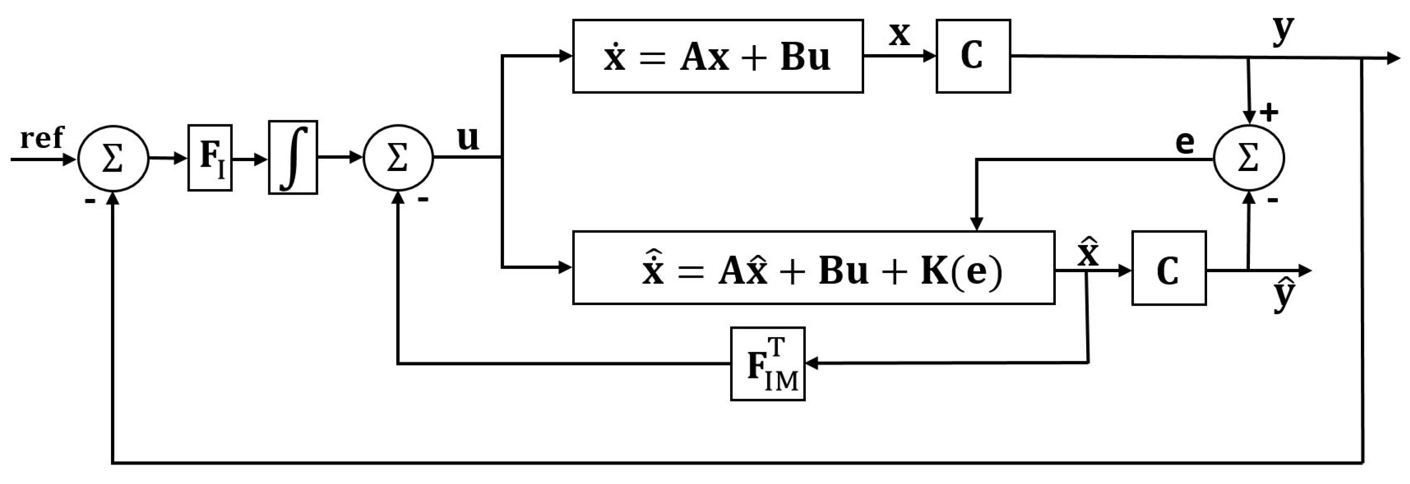
3. State Feedback Controller and Observer Design
Following the description of the augmented system, the next step is the controller and observer design. The state feedback control scheme is shown in
Figure 2 [
17]. As can be seen, the control scheme includes an integrator to improve the robustness of the controller. Further work was required to adapt the system description to the integrator such as separate
feedback gain for the separated feedback loops.
A possible solution for the LTI system controller design aims to apply the Ljapunov stability theorem [
20], i.e.,
if there exists a common positive definite matrix such as
To apply the Ljapunov stability theorem to (
21), two separated in-equations must be formulated and solved to achieve an asymptotically stable system, i.e.,
Substituting (
22) into (
24) and (
25) leads to
The following notation has been introduced in order to apply the Schur complement method [
21]
where
and
are invertible block matrices. Breaking the parenthesis in (
26) and (
27) results
Applying (
28) notation to (
29) and (
30) leads to
Multiplying the equations containing
with
and introducing
as
gives
Finally, introducing
and
and applying them to (
33) leads to the implementable form of the LMI, such as
For a more sophisticated and detailed controller design, the decay rate and input signal limitation can be implemented with the following LMIs instead of (
35)
4. Creating a Simulation Environment
After the successful formulation of the controller, the equations must be implemented in a simulation environment. In this case, MATLAB and Simulink have been used. TP toolbox [
22], SeDuMi 1.3 [
23], and Yalmip [
24] have been used for modeling and LMI solving. Observer design is not included in these tool-kits; the existing functions have been modified as shown in in Algorithm 1 for asymptotic stabilization with a decay rate [
14].
| Algorithm 1 Asymptotically stable LMI-based controller and observer design with decay rate. |
function = lmi_asym_obs(, ) fordo = reshape(A(r,:,:), [n n]) = reshape(B(r,:,:), [n m]); = reshape(C(r,:,:), [m n]); end for fordo for do = reshape(A(r,:,:), [n n]); = reshape(A(s,:,:), [n n]); = reshape(B(r,:,:), [n m]); = reshape(B(s,:,:), [n m]); = reshape(C(r,:,:), [m n]); = reshape(C(s,:,:), [m n]); end for end for
|
The implementation of (
37) is also required, which is made as shown in Algorithm 2 [
14].
| Algorithm 2 Applying input contraint to LMI-based controller and observer design. |
function = lmi_input_obs(, , ) = + [ * < ]; = + [ * < ]; fordo = + [; eye() > 0]; = + [; eye() > 0]; end for
|
The primary goal of the simulations is to create an application that can also be used in a real physical system in the future. This is why it is necessary to ensure that the simulation environment contains the best possible representation of the real environment. For this reason, Simulink is used, where an environment closer to reality was created, while in MATLAB, the simulation environment is initialized, the TP model is set up, the LMIs are solved, and data are post-processed. The following cases have been examined in Simulink:
Load-torque investigation,
Parameter-uncertainties studies,
Noise-signal implementation.
5. Simulation Results
The behavior of the designed control algorithm has been tested separately under different conditions while also applying the distractions. A detailed investigation can be performed by using Simulink, where Clark and Park transformations have been implemented to check the robustness of the controller with loads in different directions, while measurement noise has been applied and the model nominal values have been modified. The reference value for all the simulations are Wb for the direct rotor flux component and rad/s for the mechanical speed, respectively.
5.1. Applying Load Torque
One of the most common investigations of the controller behavior is to apply an external torque for a rotating machine model in the course of the speed control mode. The motor nominal torque is 2 Nm; therefore, the absolute value of
varies under that limit. The step response function can be seen in
Figure 3. The biggest overshoot of the controller happens after
as 4.47 rad/s (4.47%), where
Nm.
From the observer point of view, the observed state variables have been initialized as
. As expected, the transient error of the observer goes to zero very quickly; it takes around 2 ms, as shown in
Figure 4. Applying
does not cause an error between the motor and the observer variables. The same
profile has been applied in further simulations.
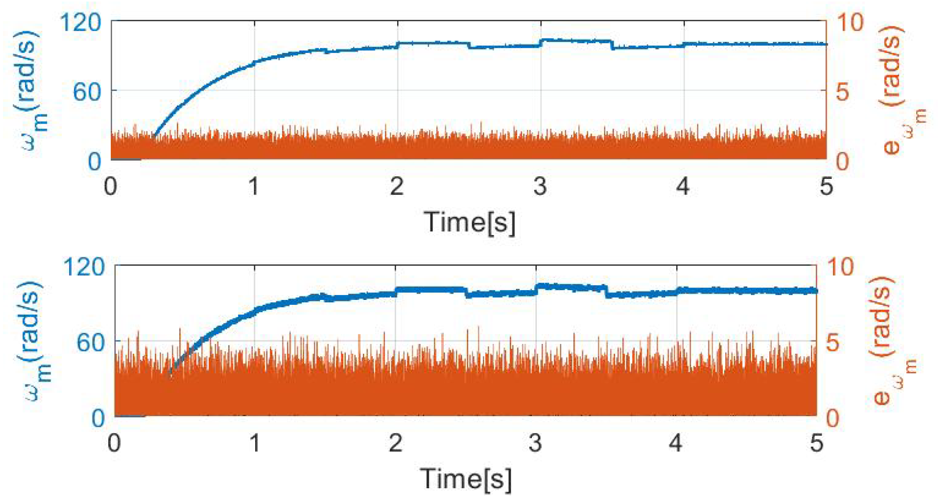
5.2. Applying Measurement Noise
In order to prepare the controller for a real environment operation, it is necessary to investigate the phenomenon of measurement noise. In this case, first the Gaussian noise signal has been added to the current signals; then, it has been applied to the feedback speed signal as well. Two different noise variances have been set and quantified: 0.001 and 0.005. While 0.001 provides a more realistic environment, 0.005 can only occur in a very noisy environment. The noise signals are shown in
Figure 5.
It must be noted that no filter has been used because it would make it more difficult to investigate the limitation of the controller. The output of a well applied filter would be less noisy than that of the implemented ones. Let us first apply the noise signal only to the measured currents. The simulation results are shown in
Figure 6, where the orange signal is the absolute error value of the observed speed and the blue curves are the step responses of the speed controller.
Even if the error scales up with the noise signal, the speed controller remains stable and reliable. The signals
and
associated with
Figure 6 can be seen in
Figure 7.
Investigating the second case, where noise has been applied to the feedback speed signal, with the amplitude of 20 times as shown in
Figure 5. Other parameters are unchanged; the results can be seen in
Figure 8 and
Figure 9.
From the current point of view, the noise amplitudes have slightly increased, but this has no effect on the control ability. The biggest difference can be observed in the error amplitudes, which are shown in
Table 1. With noise signal variance of 0.001, the mean of the error increased by 0.5034 rad/s (2721%), with a variance of 0.005 the increase is 1.125 rad/s (2698%). The percentage increase may mean that applying noise to the speed signal would cause a fatal error; however, this is not the case. The error percentage compared to the full scale of the signal remains under 6% as the maximum column shows, which is fully acceptable in this case.
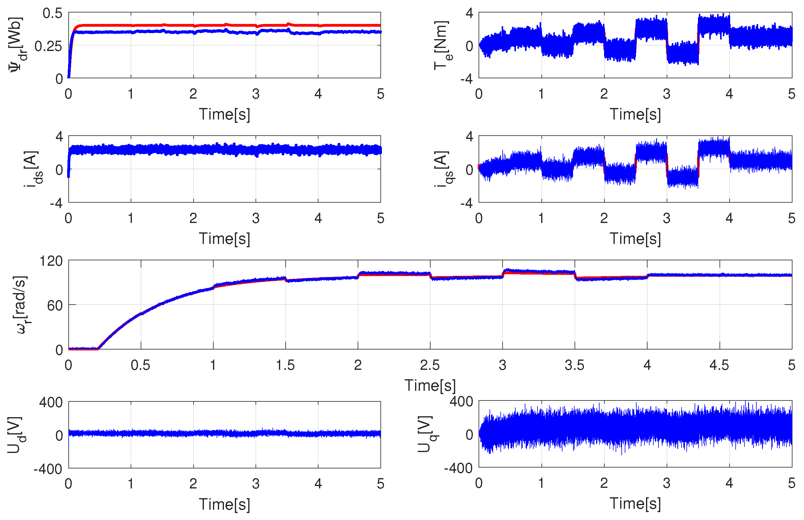
5.3. Examining Parameter Uncertainties
Investigating the behavior and stability of the controller with the tuned parameter is important, if thermal management is also taken into account. The nominal motor parameters are defined at 20 °C, while modern motors with a high power density can operate up to 180 °C. This amount of °C causes a 163% copper resistance rise. The temperature change also affects the bearing; hence, the inertia and the coefficient of the friction modification is also considerable. In order to push the controller to its limits, the following modifications have been performed in further simulations: 163% for and ; 90% for , , and ; and 130% for . Let us investigate the following setups:
The ideal condition compared with tuned parameters, applied at
(see
Figure 10),
The ideal condition compared with tuned parameters and measurement noise with a variance of 0.005 on currents, applied at
(see
Figure 11),
The ideal condition compared with tuned parameters and measurement noise with a variance of 0.001 on currents and speed, applied at
(see
Figure 12),
The ideal condition compared with tuned parameters and measurement noise with variance of 0.005 on currents and speed, applied at
(see
Figure 13).
Figure 10.
Case 1, parameter uncertainty test compared to ideal condition. Red curves with nominal parameters, blue ones with tuned.
Figure 10.
Case 1, parameter uncertainty test compared to ideal condition. Red curves with nominal parameters, blue ones with tuned.
Figure 11.
Case 2, parameter uncertainty test compared to ideal condition. Red curves with nominal parameters, blue ones with tuned.
Figure 11.
Case 2, parameter uncertainty test compared to ideal condition. Red curves with nominal parameters, blue ones with tuned.
Figure 12.
Case 3, parameter uncertainty test compared to ideal condition. Red curves with nominal parameters, blue ones with tuned.
Figure 12.
Case 3, parameter uncertainty test compared to ideal condition. Red curves with nominal parameters, blue ones with tuned.
Figure 13.
Case 4, parameter uncertainty test compared to ideal condition. Red curves with nominal parameters, blue ones with tuned.
Figure 13.
Case 4, parameter uncertainty test compared to ideal condition. Red curves with nominal parameters, blue ones with tuned.
Analyzing the similarities among the four cases, it is obvious that there is a significant difference in flux control. The explanation for the discrepancy is to be found in the determination of the flux ref, namely,
, where
is a feedback value. If
has been modified to 90% its nominal value, the controller cannot compensate for this difference because
is not measurable or observable accurately. The main goal of the controller is to provide precise speed control. The flux difference has been compensated for with increased
current. The error of the speed control has been investigated in
Figure 14. The average absolute errors of the four cases are 1.1293, 1.1787, 1.1688, and 1.2979, respectively, while the maximum errors are 3.9037, 4.3555, 4.5747, and 5.6725. The growing amount of the noise level increases the error of the speed controller, which is acceptable. As a reminder, the real-time application must contain noise filters, which results in less noisy signal than investigated in this section. Examining the
voltage signals, it can be stated that the limitation of the speed regulation will be on the side of the power electronics. As the control algorithm always finds a proper
and
excitation signal, the real question during real-time testing will be feasibility from the point of view of the electronics side. These results seem to justify the implementation of the appropriate filter algorithm.
6. Conclusions
The first part of the article has discussed the TP modeling of induction machines and its description in the form of LMI. The main section has examined the mathematical formalism of the LMI-based observer design and its implementation in a simulation environment. The primary objective in tuning the controller was to ensure robust operation, which in all cases results in a certain level of degradation of the dynamic characteristics. Consequently, it is possible to find a controller with better dynamic behavior in the literature where robustness was not considered as a criterion.
The designed controller ensures stable and accurate operation over the full operating range of the machine, taking into account the wide range of temperature values, and possible variations in inductances, which are outside the range of the parameters under consideration. The simulation results have been presented in detail, and the behavior of the nonlinear controller has been analyzed using external perturbations and measurement noises. The results of the parameter-uncertainty studies have shown that the designed controller may be suitable for testing in a real-time application. Compared to the commonly used PI current regulators, the nonlinear controller provides a more robust, accurate, and faster operation. The results presented here are difficult to compare with similar Takagi-Sugenou or LPV technics. The description of induction machines in different papers with different state-space models does not allow for a numerical comparison of the controllers. A future plan is to develop a sensorless controller algorithm by replacing the angular velocity in the feedback loop. With this condition, a comparison between the presented LMI-based observer and other model-based observers will be comparative.
Author Contributions
Conceptualization, Z.N. and M.K.; methodology, Z.N.; software, Z.N.; validation, Z.N.; formal analysis, Z.N.; investigation, Z.N.; resources, Z.N.; writing—original draft preparation, Z.N.; writing—review and editing, Z.N. and M.K.; visualization, Z.N.; and supervision, M.K. All authors have read and agreed to the published version of the manuscript.
Funding
This research received no external funding.
Institutional Review Board Statement
Not applicable.
Informed Consent Statement
Not applicable.
Data Availability Statement
Not applicable.
Conflicts of Interest
The authors declare no conflict of interest.
References
- Casadei, D.; Profumo, F.; Serra, G.; Tani, A. FOC and DTC: Two viable schemes for induction motors torque control. IEEE Trans. Power Electron. 2002, 17, 779–787. [Google Scholar] [CrossRef]
- Talla, J.; Leu, V.Q.; Šmídl, V.; Peroutka, Z. Adaptive Speed Control of Induction Motor Drive With Inaccurate Model. IEEE Trans. Ind. Electron. 2018, 65, 8532–8542. [Google Scholar] [CrossRef]
- Zou, J.; Xu, W.; Zhu, J.; Liu, Y. Low-Complexity Finite Control Set Model Predictive Control With Current Limit for Linear Induction Machines. IEEE Trans. Ind. Electron. 2018, 65, 9243–9254. [Google Scholar] [CrossRef]
- Yang, Z.; Zhang, D.; Sun, X.; Ye, X. Adaptive Exponential Sliding Mode Control for a Bearingless Induction Motor Based on a Disturbance Observer. IEEE Access 2019, 6, 35425–35434. [Google Scholar] [CrossRef]
- Zuo, Y.; Ge, X.; Chang, Y.; Chen, Y.; Xie, D.; Wang, H.; Woldegiorgis, A.T. Current Sensor Fault-Tolerant Control for Speed-Sensorless Induction Motor Drives Based on the SEPLL Current Reconstruction Scheme. IEEE Access 2022, 1–12. [Google Scholar] [CrossRef]
- Kuczmann, M.; Horváth, K. Design of Feedback Linearization Controllers for Induction Motor Drives by using Stator Reference Frame Models. In Proceedings of the 2021 IEEE 19th International Power Electronics and Motion Control Conference (PEMC), Gliwice, Poland, 25–29 April 2021; pp. 766–773. [Google Scholar]
- Ali, S.M.N.; Hanif, A.; Hossain, M.J.; Sharma, V. An LPV H∞ Control Design for the Varying Rotor Resistance Effects on the Dynamic Performance of Induction Motors. In Proceedings of the 2018 IEEE 27th International Symposium on Industrial Electronics (ISIE), Cairns, Australia, 13–15 June 2018; pp. 114–119. [Google Scholar]
- Costa, C.A.; Nied, A.; Nogueira, F.G.; de Azambuja Turqueti, M.; Rossa, A.J.; Dezuo, T.J.M.; Barra, W. Robust Linear Parameter Varying Scalar Control Applied in High Performance Induction Motor Drives. IEEE Trans. Ind. Electron. 2021, 68, 10558–10568. [Google Scholar] [CrossRef]
- Baranyi, P. The generalized TP model transformation for TS fuzzy model manipulation and generalized stability verification. IEEE Trans. Fuzzy Syst. 2014, 22, 934–948. [Google Scholar] [CrossRef]
- Baranyi, P. Extracting LPV and qLPV Structures From State-Space Functions: A TP Model Transformation Based Framework. IEEE Trans. Fuzzy Syst. 2020, 28, 499–509. [Google Scholar] [CrossRef]
- Szollosi, A.; Baranyi, P. Influence of the Tensor Product Model Representation of qLPV Models on the Feasibility of Linear Matrix Inequality Based Stability Analysis. Asian J. Control 2017, 10, 531–547. [Google Scholar] [CrossRef]
- Németh, Z.; Kuczmann, M. Tensor product transformation-based modeling of an induction machine. Asian J. Control 2021, 23, 1280–1289. [Google Scholar] [CrossRef]
- Németh, Z.; Kuczmann, M. Tensor Product Transformation Based Robust Control of Induction Machine. In Proceedings of the 2020 2nd IEEE International Conference on Gridding and Polytope Based modeling and Control (GPMC), Budapest, Hungary, 19 November 2020; pp. 39–44. [Google Scholar]
- Tanaka, K.; Wang, H.O. Fuzzy Control Systems Design and Analysis: A Linear Matrix Inequality Approach; John Wiley & Sons, Inc.: New York, NY, USA, 2001. [Google Scholar]
- Govindasamy, N.; Syed, A.M.; Quanxin, Z.; Bandana, P.; Ganesh, T. Fuzzy observer-based consensus tracking control for fractional-order multi-agent systems under cyber-attacks and its application to electronic circuits. IEEE Trans. Netw. Sci. Eng. 2022, 1–11. [Google Scholar] [CrossRef]
- Chang, W.-J.; Tsai, M.-H.; Pen, C.-L. Observer-Based Fuzzy Controller Design for Nonlinear Discrete-Time Singular Systems via Proportional Derivative Feedback Scheme. Appl. Sci. 2021, 11, 2833. [Google Scholar] [CrossRef]
- Keviczky, L.; Bars, R.; Hetthessy, J.; Banyasz, C. Control Engineering; Springer: Cham, Switzerland, 2019. [Google Scholar]
- Baranyi, P.; Szeidl, L.; Varlaki, P.; Yam, Y. Definition of the HOSVD based canonical form of polytopic dynamic models. In Proceedings of the 2006 IEEE International Conference on Mechatronics, Luoyang, China, 25–28 June 2006; pp. 660–665. [Google Scholar]
- Szeidl, L.; Varlaki, P. HOSVD based canonical form for polytopic models of dynamic systems. J. Adv. Comput. Intell. Intell. Inform. 2009, 13, 52–60. [Google Scholar] [CrossRef]
- Feng, M.; Harris, C.J. Piecewise Lyapunov stability conditions of fuzzy systems. IEEE Trans. Syst. Man Cybern. Part (Cybern.) 2001, 31, 259–262. [Google Scholar] [CrossRef] [PubMed]
- Gaidamour, J.; Hénon, P. A Parallel Direct/Iterative Solver Based on a Schur Complement Approach. In Proceedings of the 2008 11th IEEE International Conference on Computational Science and Engineering, Washington, DC, USA, 16–18 July 2008; pp. 98–105. [Google Scholar]
- Nagy, S.Z.; Petres, Z.; Baranyi, P. TP tool—A MATLAB toolbox for TP model transformation. In Proceedings of the 8th International Symposium of Hungarian Researchers on Computational Intelligence and Informatics, CINTI 2007, Budapest, Hungary, 15–17 November 2007; pp. 483–495. [Google Scholar]
- Sturm, J.F. Using SeDuMi 1.02, a MATLAB toolbox for optimization over symmetric cones. Optim. Methods Softw. 1999, 11, 625–653. [Google Scholar] [CrossRef]
- Lofberg, J. YALMIP: A toolbox for modeling and optimization in MATLAB. In Proceedings of the 2004 IEEE International Conference on Robotics and Automation (IEEE Cat. No.04CH37508), New Orleans, LA, USA, 26 April–1 May 2004; pp. 284–289. [Google Scholar]
| Publisher’s Note: MDPI stays neutral with regard to jurisdictional claims in published maps and institutional affiliations. |
© 2022 by the authors. Licensee MDPI, Basel, Switzerland. This article is an open access article distributed under the terms and conditions of the Creative Commons Attribution (CC BY) license (https://creativecommons.org/licenses/by/4.0/).


