
Vehicle Motion Prediction Algorithm Based on Artificial Potential Field Correction and Fuzzy C-Mean Driving Intention Classification


Abstract
1. Introduction
2. Overview of Vehicle Trajectory Prediction
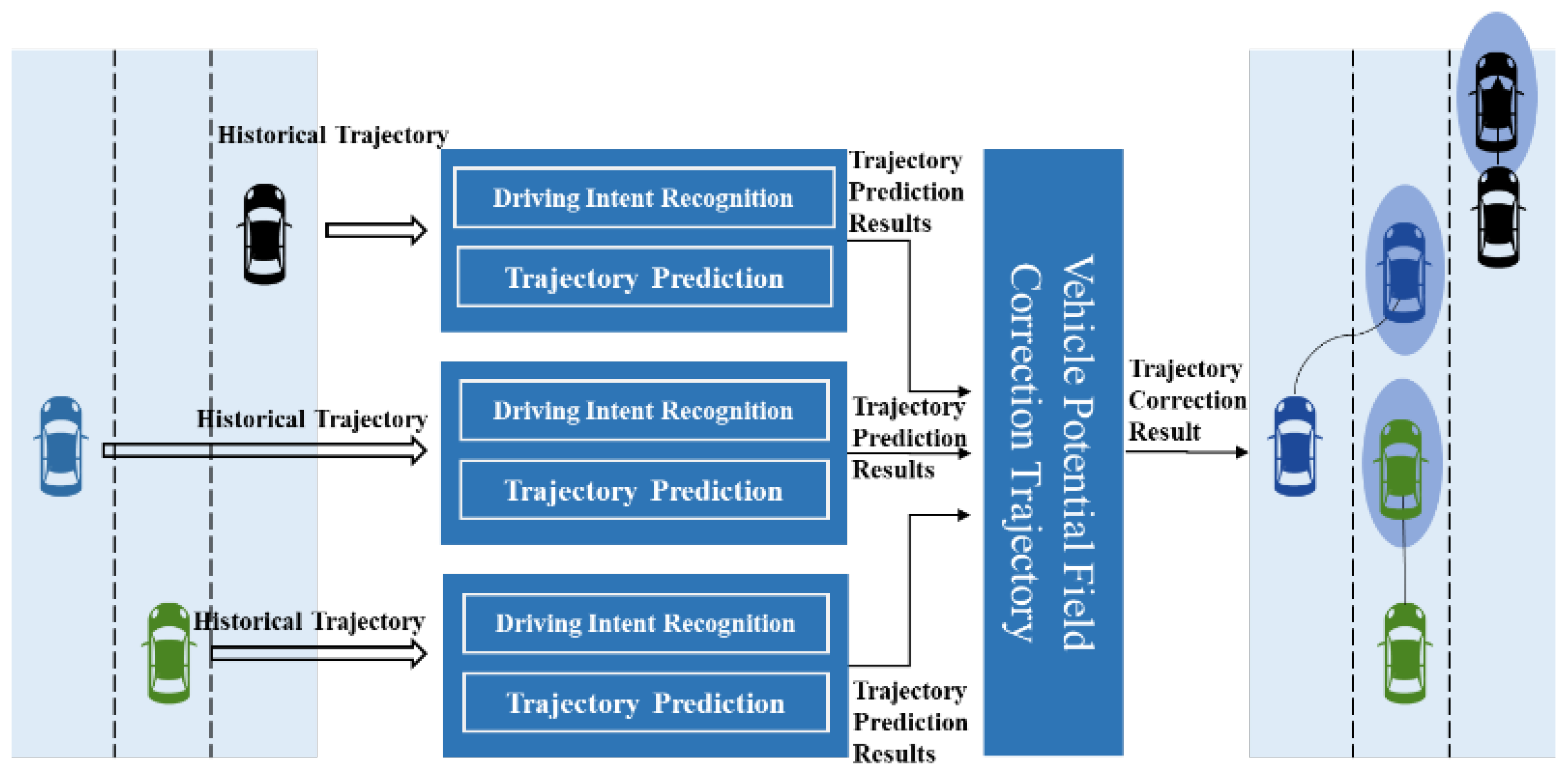
3. System Overview
3.1. Driving Intention Classification
3.2. Trajectory Prediction
3.3. Vehicle Interaction Correction
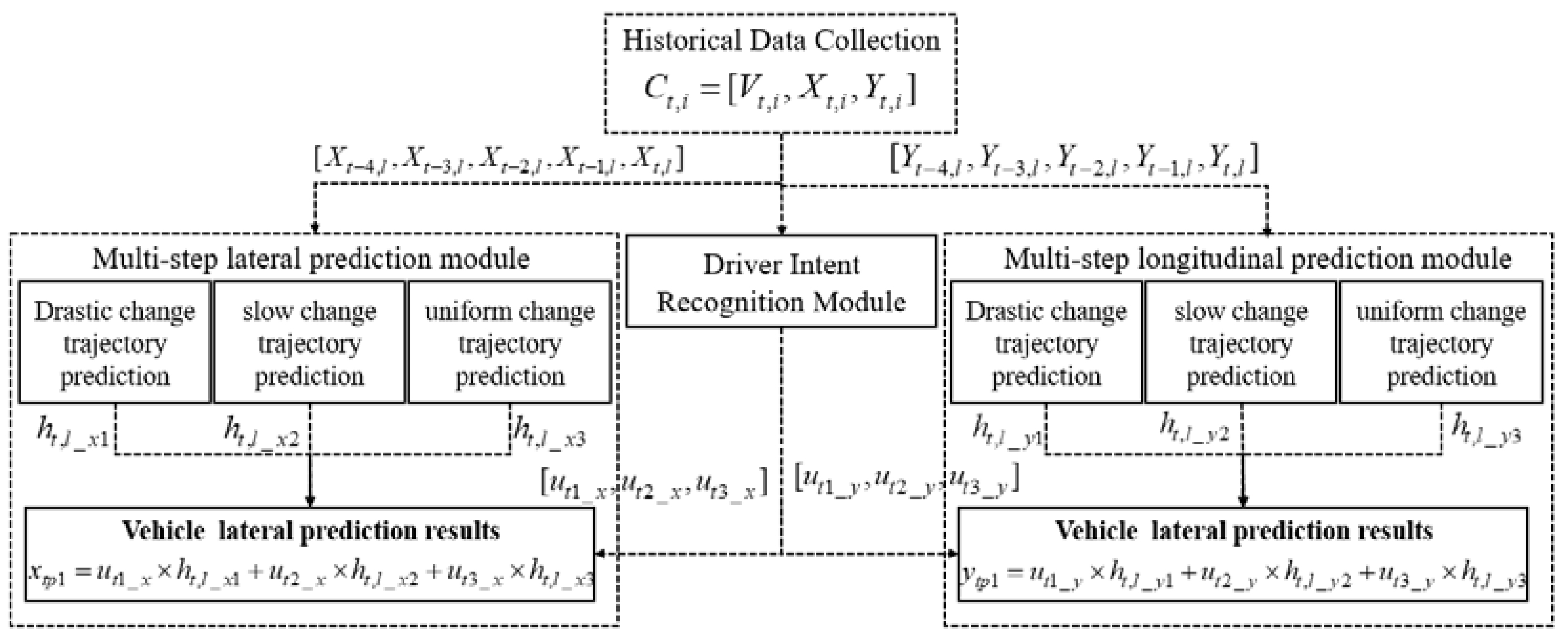
3.4. Multi-Step Prediction
4. Experimental Results and Analysis
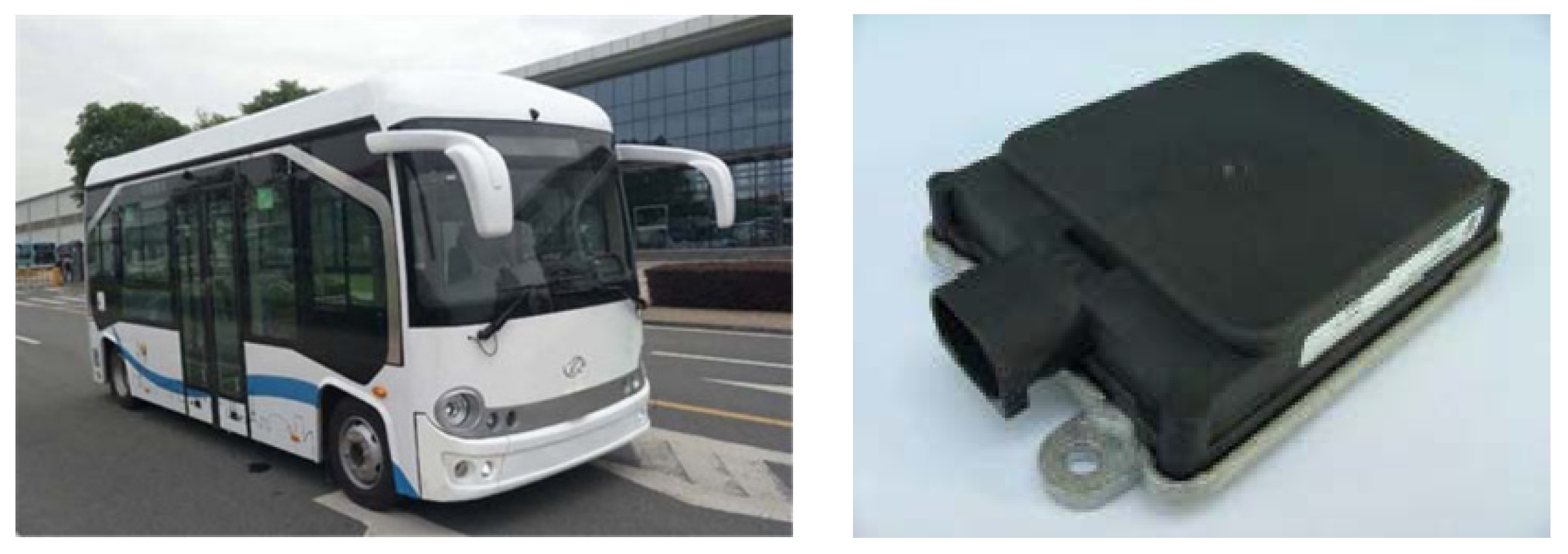
4.1. Research Subjects
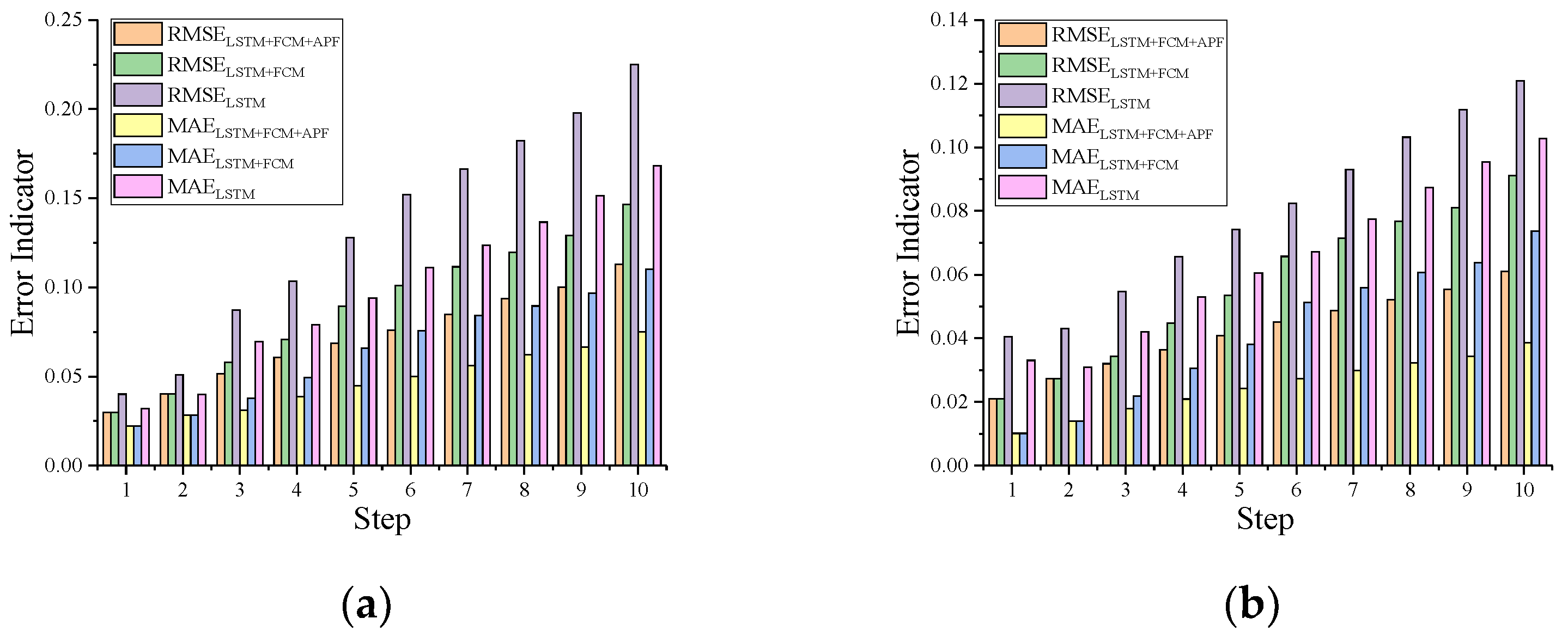
4.2. Evaluation Indicators
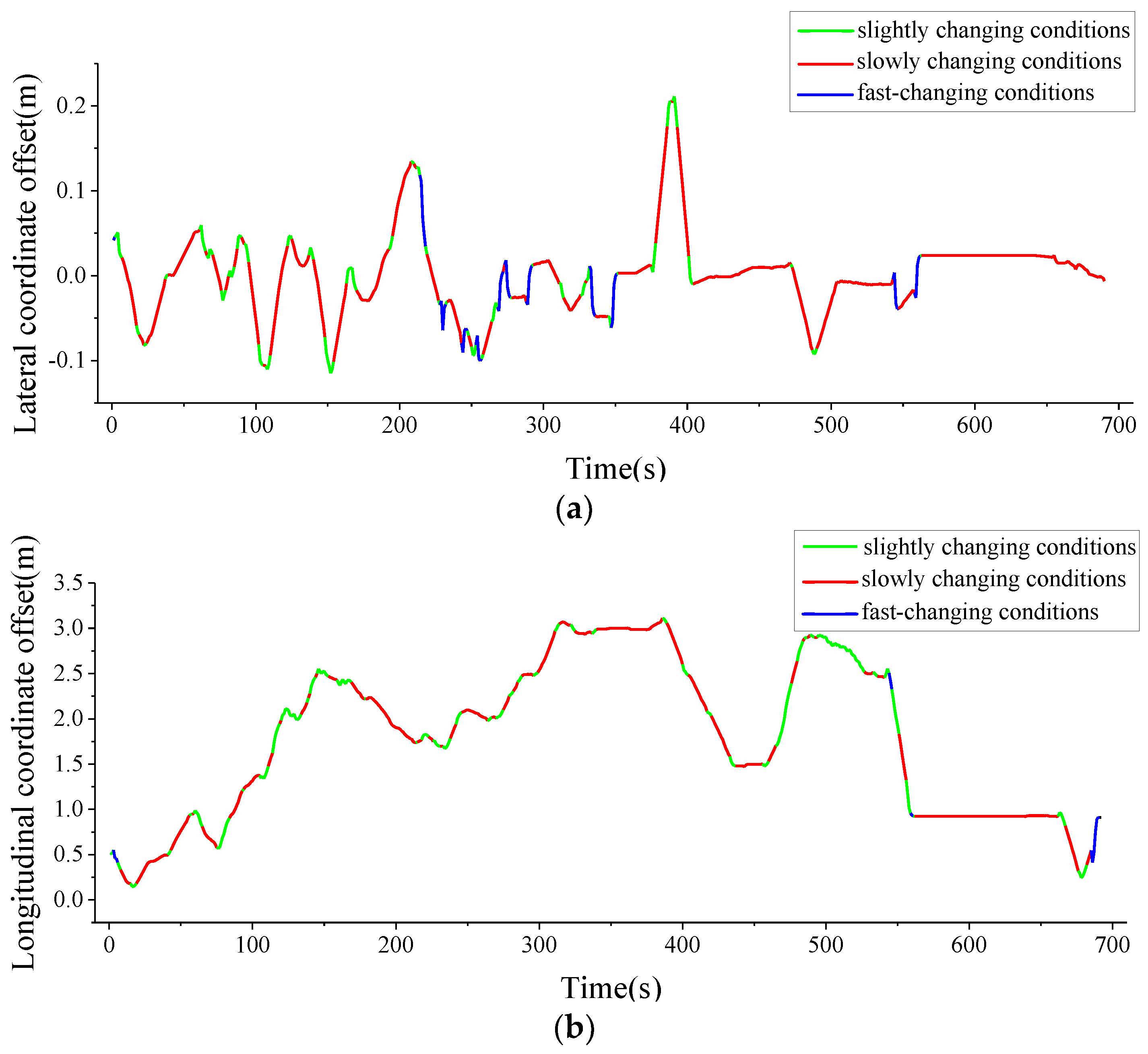
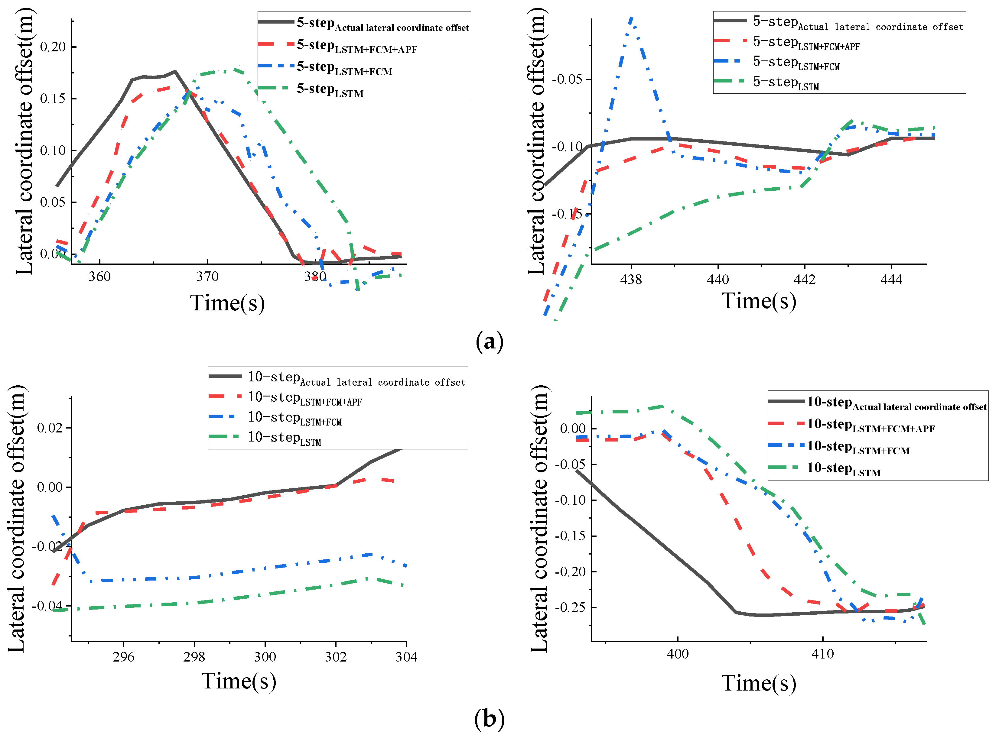
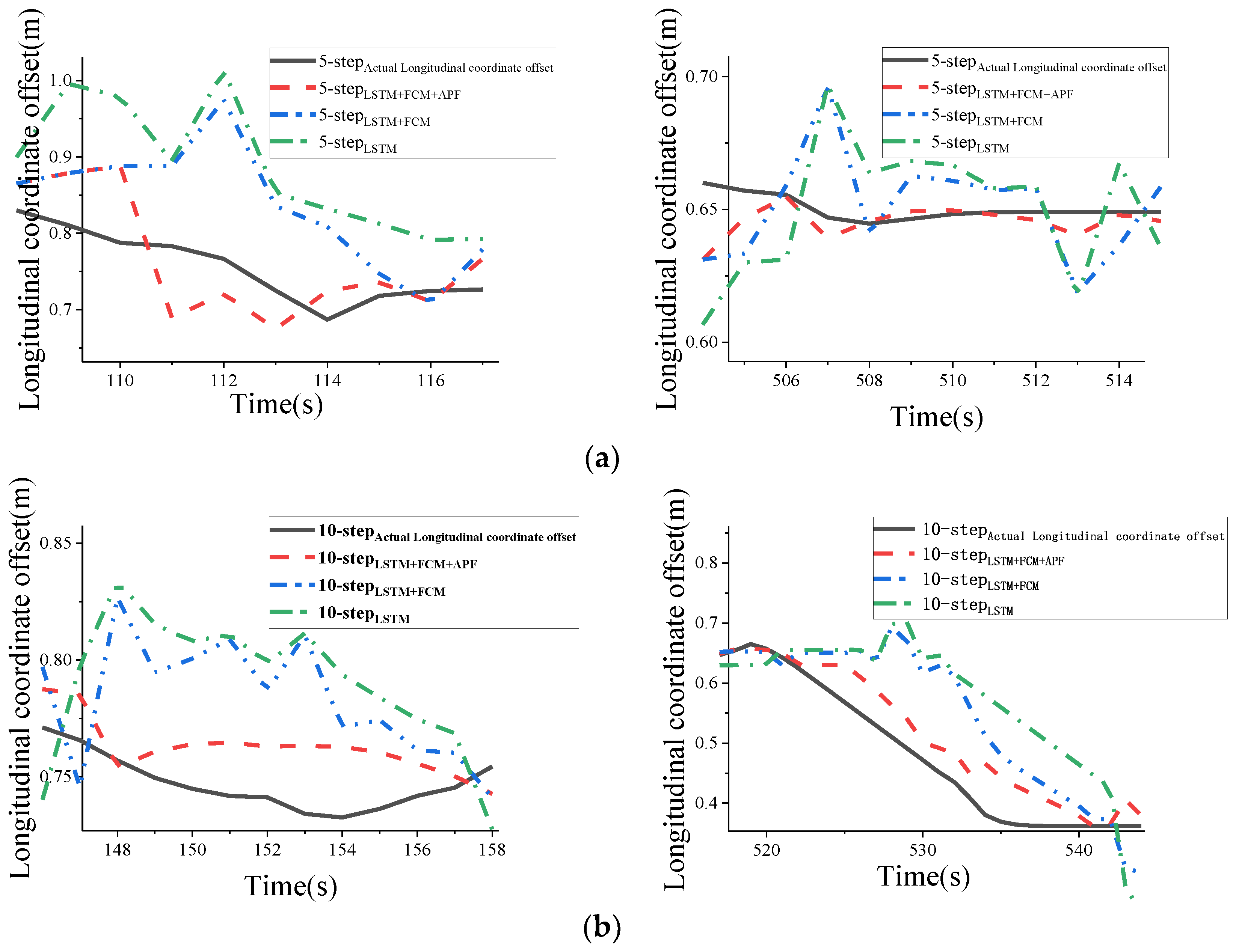
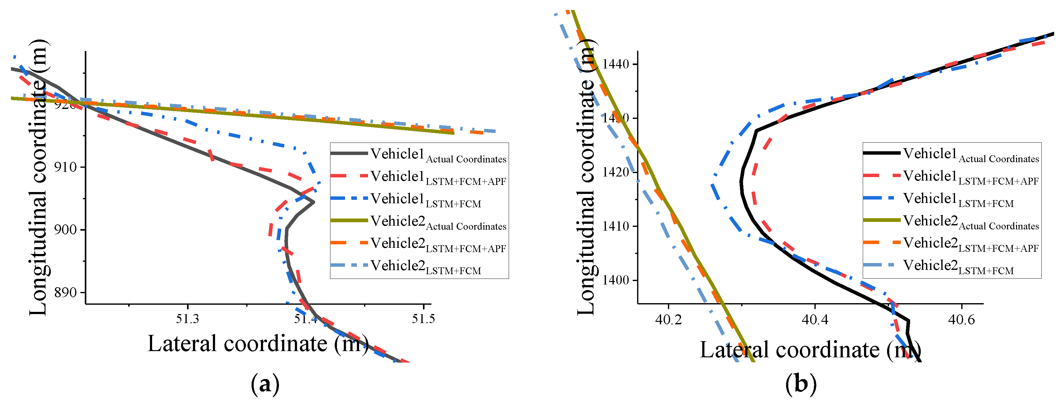
4.3. Analysis of Experimental Results
5. Conclusions
Author Contributions
Funding
Data Availability Statement
Conflicts of Interest
References
- Bello, L.L.; Mariani, R.; Mubeen, S.; Saponara, S. Recent advances and trends in on-board embedded and networked automotive systems. IEEE Trans. Ind. Inf. 2019, 15, 1038–1051. [Google Scholar] [CrossRef]
- Woo, H.; Ji, Y.; Tamura, Y.; Kuroda, Y.; Sugano, T.; Yamamoto, Y.; Yamashita, A.; Asama, H. Lane-change detection based on individual driving style. Adv. Robot. 2019, 33, 1087–1098. [Google Scholar] [CrossRef]
- Lefèvre, S.; Vasquez, D.; Laugier, C. A survey on motion prediction and risk assessment for intelligent vehicles. Robomech J. 2014, 1, 1–14. [Google Scholar] [CrossRef]
- Wasala, A.; Byrne, D.; Miesbauer, P.; O’Hanlon, J.; Heraty, P.; Barry, P. Trajectory based lateral control: A reinforcement learning case study. Eng. Appl. Artif. Intell. 2020, 94, 103799. [Google Scholar] [CrossRef]
- Dini, P.; Saponara, S. Processor-in-the-loop validation of a gradient descent-based model predictive control for assisted driving and obstacles avoidance applications. IEEE Access 2022, 10, 67958–67975. [Google Scholar] [CrossRef]
- Sharma, O.; Sahoo, N.C.; Puhan, N.B. Recent advances in motion and behavior planning techniques for software architecture of autonomous vehicles: A state-of-the-art survey. Eng. Appl. Artif. Intell. 2021, 101, 104211. [Google Scholar] [CrossRef]
- Saponara, S.; Greco, M.S.; Gini, F. Radar-on-chip/in-package in autonomous driving vehicles and intelligent transport systems: Opportunities and challenges. IEEE Signal Process. Mag. 2019, 36, 71–84. [Google Scholar] [CrossRef]
- Deo, N.; Trivedi, M.M. Convolutional social pooling for vehicle trajectory prediction. In Proceedings of the IEEE Conference on Computer Vision and Pattern Recognition Workshops, Salt Lake City, UT, USA, 18–22 June 2018; pp. 1468–1476. [Google Scholar]
- Houenou, A.; Bonnifait, P.; Cherfaoui, V.; Yao, W. Vehicle trajectory prediction based on motion model and maneuver recognition. In Proceedings of the 2013 IEEE/RSJ International Conference on Intelligent Robots and Systems, Tokyo, Japan, 3–7 November 2013; IEEE: Manhattan, NY, USA, 2013; pp. 4363–4369. [Google Scholar]
- Dai, S.; Li, L.; Li, Z. Modeling vehicle interactions via modified LSTM models for trajectory prediction. IEEE Access 2019, 7, 38287–38296. [Google Scholar] [CrossRef]
- Lin, L.; Li, W.; Bi, H.; Qin, L. Vehicle trajectory prediction using LSTMs with spatial-temporal attention mechanisms. IEEE Intel. Transp. Syst. Mag. 2021, 14, 197–208. [Google Scholar] [CrossRef]
- Rummelhard, L.; Nègre, A.; Perrollaz, M.; Laugier, C. Probabilistic Grid-Based Collision Risk Prediction for Driving Application; Experimental Robotics; Springer: Cham, Switzerland, 2016; pp. 821–834. [Google Scholar]
- Xie, G.; Gao, H.; Qian, L.; Huang, B.; Li, K.; Wang, J. Vehicle trajectory prediction by integrating physics-and maneuver-based approaches using interactive multiple models. IEEE Trans. Ind. Electron. 2017, 65, 5999–6008. [Google Scholar] [CrossRef]
- Xiao, W.; Zhang, L.; Meng, D. Vehicle trajectory prediction based on motion model and maneuver model fusion with interactive multiple models. SAE Int. J. Adv. Curr. Pract. Mobil. 2020, 2, 3060–3071. [Google Scholar]
- Baek, M.; Jeong, D.; Choi, D.; Lee, S. Vehicle trajectory prediction and collision warning via fusion of multisensors and wireless vehicular communications. Sensors 2020, 20, 288. [Google Scholar] [CrossRef] [PubMed]
- Liu, W.; He, H.; Sun, F. Vehicle state estimation based on minimum model error criterion combining with extended Kalman filter. J. Frankl. Inst. 2016, 353, 834–856. [Google Scholar] [CrossRef]
- Yoon, Y.; Kim, T.; Lee, H.; Park, J. Road-aware trajectory prediction for autonomous driving on highways. Sensors 2020, 20, 4703. [Google Scholar] [CrossRef] [PubMed]
- Yalamanchi, S.; Huang, T.K.; Haynes, G.C.; Djuric, N. Long-term prediction of vehicle behavior using short-term uncertainty-aware trajectories and high-definition maps. In Proceedings of the 2020 IEEE 23rd International Conference on Intelligent Transportation Systems (ITSC), Rhodes, Greece, 20–23 September 2020; IEEE: Manhattan, NY, USA, 2020; pp. 1–6. [Google Scholar]
- Zou, B.; Li, W.; Hou, X.; Tang, L.; Yuan, Q. A framework for trajectory prediction of preceding target vehicles in urban scenario using multi-sensor fusion. Sensors 2022, 22, 4808. [Google Scholar] [CrossRef] [PubMed]
- Li, H.; Liu, F.; Zhao, Z.; Karimzadeh, M. Effective safety message dissemination with vehicle trajectory predictions in V2X networks. Sensors 2022, 22, 2686. [Google Scholar] [CrossRef] [PubMed]
- Qu, D.; Wang, S.; Liu, H.; Meng, Y. A car-following model based on trajectory data for connected and automated vehicles to predict trajectory of human-driven vehicles. Sustainability 2022, 14, 7045. [Google Scholar] [CrossRef]
- Wang, J.; Wang, P.; Zhang, C.; Su, K.; Li, J. F-net: Fusion neural network for vehicle trajectory prediction in autonomous driving. In Proceedings of the ICASSP 2021—2021 IEEE International Conference on Acoustics, Speech and Signal Processing (ICASSP), Toronto/Ontario, Canada, 6–11 June 2021; IEEE: Manhattan, NY, USA, 2021; pp. 4095–4099. [Google Scholar]
- Choi, D.; Yim, J.; Baek, M.; Lee, S. Machine learning-based vehicle trajectory prediction using v2v communications and on-board sensors. Electronics 2021, 10, 420. [Google Scholar] [CrossRef]
- Shen, C.H.; Hsu, T.J. Research on vehicle trajectory prediction and warning based on mixed neural networks. Appl. Sci. 2020, 11, 7. [Google Scholar] [CrossRef]
- Lv, P.; Liu, H.; Xu, J.; Li, T. Trajectory prediction with correction mechanism for connected and autonomous vehicles. Electronics 2022, 11, 2149. [Google Scholar] [CrossRef]
- Zhao, T.; Xu, Y.; Monfort, M.; Choi, W.; Baker, C.; Zhao, Y.; Wang, Y.; Wu, Y.N. Multi-agent tensor fusion for contextual trajectory prediction. In Proceedings of the IEEE/CVF Conference on Computer Vision and Pattern Recognition, Long Beach, CA, USA, 15–20 June 2019; pp. 12126–12134. [Google Scholar]
- Yu, D.; Lee, H.; Kim, T.; Hwang, S.H. Vehicle trajectory prediction with lane stream attention-based LSTMs and road geometry linearization. Sensors 2021, 21, 8152. [Google Scholar] [CrossRef] [PubMed]
- Jo, E.; Sunwoo, M.; Lee, M. Vehicle trajectory prediction using hierarchical graph neural network for considering interaction among multimodal maneuvers. Sensors 2021, 21, 5354. [Google Scholar] [CrossRef] [PubMed]
- Li, J.; Ma, H.; Zhan, W.; Tomizuka, M. Coordination and trajectory prediction for vehicle interactions via Bayesian generative modeling. In Proceedings of the 2019 IEEE Intelligent Vehicles Symposium (IV), Paris, France, 9–12 June 2019; IEEE: Manhattan, NY, USA, 2019; pp. 2496–2503. [Google Scholar]
- Robicquet, A.; Sadeghian, A.; Alahi, A.; Savarese, S. Learning social etiquette: Human trajectory understanding in crowded scenes. In Proceedings of the European Conference on Computer Vision, Odessa, Ukraine, 6 July 2019; Springer: Cham, Switzerland, 2016; pp. 549–565. [Google Scholar]
- Park, S.H.; Lee, G.; Seo, J.; Bhat, M.; Kang, M.; Francis, J.; Jadhav, A.; Liang, P.P.; Morency, L.-P. Diverse and admissible trajectory forecasting through multimodal context understanding. In Proceedings of the European Conference on Computer Vision, Glasgow, UK, 23–28 August 2020; Springer: Cham, Switzerland, 2020; pp. 282–298. [Google Scholar]
- Cosimi, F.; Dini, P.; Giannetti, S.; Petrelli, M.; Saponara, S. Analysis and design of a non-linear MPC algorithm for vehicle trajectory tracking and obstacle avoidance. In Applications in Electronics Pervading Industry, Environment and Society; Saponara, S., de Gloria, A., Eds.; ApplePies 2020; Lecture Notes in Electrical Engineering; Springer: Cham, Switzerland, 2020; Volume 738. [Google Scholar] [CrossRef]
- Zyner, A.; Worrall, S.; Ward, J.; Nebot, E. Long short term memory for driver intent prediction. In Proceedings of the 2017 IEEE Intelligent Vehicles Symposium (IV), Los Angeles, CA, USA, 11–14 June 2017; IEEE: Manhattan, NY, USA, 2017; pp. 1484–1489. [Google Scholar]
- Zyner, A.; Worrall, S.; Nebot, E. A recurrent neural network solution for predicting driver intention at unsignalized intersections. IEEE Robot. Automat. Lett. 2018, 3, 1759–1764. [Google Scholar] [CrossRef]
- Lee, D.; Kwon, Y.P.; McMains, S.; Hedrick, J.K. Convolution neural network-based lane change intention prediction of surrounding vehicles for ACC. In Proceedings of the 2017 IEEE 20th International Conference on Intelligent Transportation Systems (ITSC), Yokohama, Japan, 16–19 October 2017; IEEE: Manhattan, NY, USA, 2017; pp. 1–6. [Google Scholar]
- Liu, L.; Xu, G.; Song, Z. Driver lane changing behavior analysis based on parallel Bayesian networks. In Proceedings of the 2010 Sixth International Conference on Natural Computation, Yantai, China, 10–12 August 2010; IEEE: Manhattan, NY, USA, 2010; Volume 3, pp. 1232–1237. [Google Scholar]
- Mozaffari, S.; Al-Jarrah, O.Y.; Dianati, M.; Jennings, P.; Mouzakitis, A. Deep learning-based vehicle behavior prediction for autonomous driving applications: A review. IEEE Trans. Intell. Transp. Syst. 2020, 23, 33–47. [Google Scholar] [CrossRef]
- Wang, X.; Wang, H. Driving behavior clustering for hazardous material transportation based on genetic fuzzy C-means algorithm. IEEE Access 2020, 8, 11289–11296. [Google Scholar] [CrossRef]
- Liu, Y.; Wang, J.; Zhao, P.; Qin, D.; Chen, Z. Research on classification and recognition of driving styles based on feature engineering. IEEE Access 2019, 7, 89245–89255. [Google Scholar] [CrossRef]
- Olsen, E.C.B. Modeling Slow Lead Vehicle Lane Changing. Ph.D. Thesis, Virginia Polytechnic Institute and State University, Blacksburg, VA, USA, 2003. [Google Scholar]
- Graves, A. Long Short-Term Memory. Neural Comput. 1997, 9, 1735–1780. [Google Scholar]
- Corso, A.; Du, P.; Driggs-Campbell, K.; Kochenderfer, M.J. Adaptive stress testing with reward augmentation for autonomous vehicle validation. In Proceedings of the 2019 IEEE Intelligent Transportation Systems Conference (ITSC), Auckland, New Zealand, 27–30 October 2019; pp. 163–168. [Google Scholar] [CrossRef]
- Girard, A.; Rasmussen, C.E.; Quinonero-Candela, J.; Murray-Smith, R.; Winther, O.; Larsen, J. Multiple-step ahead prediction for non linear dynamic systems—A gaussian process treatment with propagation of the uncertainty. Adv. Neural Inf. Process. Syst. 2002, 15, 529–536. [Google Scholar]
- Hachino, T.; Kadirkamanathan, V. Time series forecasting using multiple gaussian process prior model. In Proceedings of the 2007 IEEE Symposium on Computational Intelligence and Data Mining, Honolulu, HI, USA, 1 March–5 April 2007; IEEE: Manhattan, NY, USA, 2007; pp. 604–609. [Google Scholar]
- Yan, W.; Qiu, H.; Xue, Y. Gaussian process for long-term time-series forecasting. In Proceedings of the 2009 International Joint Conference on Neural Networks, Atlanta, GA, USA, 14–19 June 2009; IEEE: Manhattan, NY, USA, 2009; pp. 3420–3427. [Google Scholar]


| No. | Characteristic Parameters |
|---|---|
| 1 | Vehicle speed (m/s) |
| 2 | Lateral coordinate relative maximum offset (m) |
| 3 | Lateral coordinate relative minimum offset (m) |
| 4 | Longitudinal coordinate relative maximum offset (m) |
| 5 | Longitudinal coordinate relative minimum offset (m) |
| Parameter | |
|---|---|
| Length (mm) | 6605 |
| Width (mm) | 2320 |
| Height (mm) | 2870 |
| Maximum Speed (km/h) | 69 |
| Prediction Algorithms | Mean Value | Variance |
|---|---|---|
| LSTM + FCM + APF | 0.022367 | 0.000753 |
| LSTM + FCM | 0.03478 | 0.001322 |
| LSTM | 0.054549 | 0.002092 |
| Prediction Algorithms | Mean Value | Variance |
|---|---|---|
| LSTM + FCM + APF | 0.035086 | 0.001718 |
| LSTM + FCM | 0.054699 | 0.00277 |
| LSTM | 0.084863 | 0.008036 |
| Prediction Algorithms | Mean Value | Variance |
|---|---|---|
| LSTM + FCM + APF | 0.006113 | 5.02 × 10⁻⁵ |
| LSTM + FCM | 0.008988 | 6.8 × 10⁻⁵ |
| LSTM | 0.012833 | 0.000141 |
| Prediction Algorithms | Mean Value | Variance |
|---|---|---|
| LSTM + FCM + APF | 0.029771 | 0.001118 |
| LSTM + FCM | 0.043256 | 0.00147 |
| LSTM | 0.067788 | 0.003272 |
Publisher’s Note: MDPI stays neutral with regard to jurisdictional claims in published maps and institutional affiliations. |
© 2022 by the authors. Licensee MDPI, Basel, Switzerland. This article is an open access article distributed under the terms and conditions of the Creative Commons Attribution (CC BY) license (https://creativecommons.org/licenses/by/4.0/).
Share and Cite
Ma, W.; Zhu, Y.; Wu, Z. Vehicle Motion Prediction Algorithm Based on Artificial Potential Field Correction and Fuzzy C-Mean Driving Intention Classification. Electronics 2022, 11, 3857. https://doi.org/10.3390/electronics11233857
Ma W, Zhu Y, Wu Z. Vehicle Motion Prediction Algorithm Based on Artificial Potential Field Correction and Fuzzy C-Mean Driving Intention Classification. Electronics. 2022; 11(23):3857. https://doi.org/10.3390/electronics11233857
Chicago/Turabian StyleMa, Wenda, Yuan Zhu, and Zhihong Wu. 2022. "Vehicle Motion Prediction Algorithm Based on Artificial Potential Field Correction and Fuzzy C-Mean Driving Intention Classification" Electronics 11, no. 23: 3857. https://doi.org/10.3390/electronics11233857
APA StyleMa, W., Zhu, Y., & Wu, Z. (2022). Vehicle Motion Prediction Algorithm Based on Artificial Potential Field Correction and Fuzzy C-Mean Driving Intention Classification. Electronics, 11(23), 3857. https://doi.org/10.3390/electronics11233857