Wide-Speed-Range Sensorless Control of IPMSM

Abstract

A wide-speed-range sensorless control for an IPMSM is deeply studied in this paper, which combines the high-frequency injection (HFI) method and sliding-mode observer (SMO) method. At low-speed range, a rotating high-frequency voltage signal is injected into the IPMSM; the rotor position can be estimated by the HFI method based on the saliency of the IPMSM. At high-speed range, an SMO method based on the extended back electromotive force (EMF) of the IPMSM is utilized to estimate the rotor position. Furthermore, to blend the positions estimated by these two methods, a speed-dependent weight function is designed. The steady-state and dynamic performance of the wide-speed sensorless control are investigated by experiments. In high-speed range, the position estimation errors of the SMO method at different operation points are smaller than 6 el.deg.; in low-speed range, the position estimation errors of the HFI method at different operation points are smaller than 15 el.deg.; and during the transition process, the IPMSM can switch smoothly between the HFI-based and SMO-based sensorless control methods.

1. Introduction

Sensorless control methods can be classified into two categories: the fundamental-model-based methods for high-speed range and the saliency-based methods for low-speed range. The fundamental-model-based methods are available in the medium- and high-speed ranges, while the saliency-based methods are able to track the position at standstill and low-speed ranges [1,2,3,4].

For the fundamental-model-based methods, the rotor position is normally detected by estimating the back electromotive force (EMF). Since the amplitude of the back EMF is proportional to rotor speed, the fundamental-model-based methods would fail in the low-speed range due to the low signal-to-noise ratio (SNR). To estimate the rotor position in the low-speed range, the saliency-based methods are developed, which are also known as high-frequency injection (HFI) methods. In these methods, a high-frequency voltage signal is injected into an IPMSM. Due to the saliency effect of the IPMSM, the corresponding high-frequency current response is modulated by the rotor position. Therefore, the rotor position can be extracted from the high-frequency current response. However, with the increase in rotor speed, the frequency of the back EMF comes close to the frequency of the injected high-frequency signal. Then, the rotor position contained in the high-frequency current response is seriously interfered by the EMF in high-speed range. Consequently, for wide-speed-range sensorless control, it is common to combine the saliency-based method and the fundamental-model-based method and utilize the two methods in low-speed and high-speed ranges, respectively.

Referring to the fundamental-model-based methods, they can be implemented either in the $\alpha \beta$ frame or $dq$ frame. In the $dq$ frame, the model reference adaptive system (MRAS) can be utilized to estimate the rotor position [5,6]. For the fundamental-model-based methods implemented in the $\alpha \beta$ frame, the conventional voltage model of the IPMSM cannot be utilized directly, since the information of rotor position is contained not only in the back EMF but also in the inductance matrix. To solve this problem, some new voltage models of the IPMSM in $\alpha \beta$ frame are proposed. An extended EMF model is proposed in [7]. Additionally, the active flux model is proposed in [8,9].

The fundamental-model-based methods in the $\alpha \beta$ frame mainly include the flux observer method [10], the extended Kalman filter (EKF) method [11,12], the sliding-mode observer (SMO) method [13,14,15], etc. Due to the advantages of fast response and strong robustness to disturbance and parameters variation, the SMO method has been widely used in practical applications. The SMO method is essentially a kind of nonlinear control method, which utilizes a nonlinear SMO control function, such as sign function, to force the estimated current value to converge to the actual value. Then, the rotor position can be extracted from the output signal of the SMO control function. However, the chattering problem caused by the SMO control function would deteriorate the performance of position estimation. This could be mitigated by choosing the proper parameters of the SMO control function.

Referring to the saliency-based methods for low-speed ranges, according to the injected signal, the saliency-based methods can be classified into rotating-voltage injection method [16,17,18], pulsating-voltage injection method [19,20,21], square-wave voltage injection method [22,23,24], and fundamental pulse width modulation (PWM) excitation-based method [25,26,27,28,29,30,31,32]. In this paper, the most commonly used rotating-voltage injection method is adopted. For the rotating-voltage injection method, a high-frequency rotating voltage vector is injected into the motor in the $\alpha \beta$ frame. In the corresponding high-frequency current response, the phase angle of the negative-sequence component contains the information of rotor position. However, the injected high-frequency signal inevitably generates torque ripples and acoustic noises.

In order to combine the fundamental-model-based method with the saliency-based method to realize sensorless control in wide-speed range, a suitable transition algorithm between the low-speed and high-speed sensorless control is required. In this paper, a speed-dependent weighting function [14,30,33] is adopted to blend these two estimated position signals. This algorithm is simple, effective, and widely utilized for the transition process of sensorless control.

In this paper, to realize the wide-speed-range sensorless control, the rotating voltage HFI method is utilized for rotor position estimation in low-speed range, and the SMO method is chosen for rotor position estimation in high-speed range. In addition, in order to seamlessly switch between the low-speed sensorless and high-speed sensorless methods, a speed-dependent weight function is adopted to blend the rotor positions estimated by these two methods. The steady-state and dynamic performance of the HFI method and the SMO method are all fully investigated by experiment. Then, after combining these two methods, the wide-speed sensorless control method is validated by the dynamic experiments.

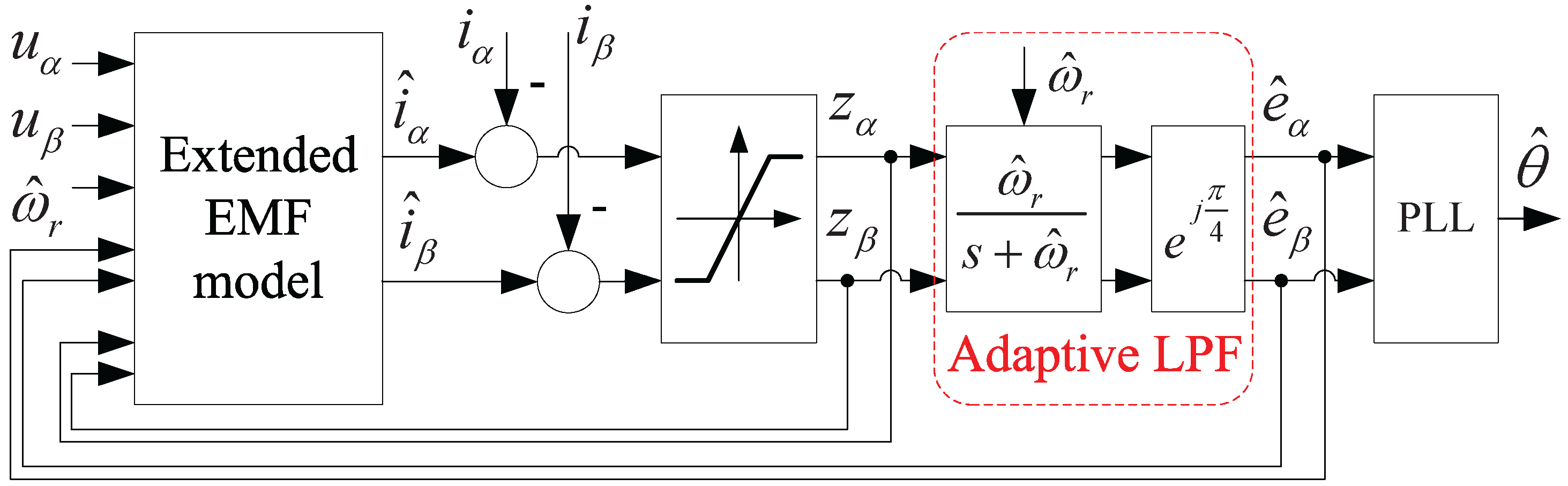
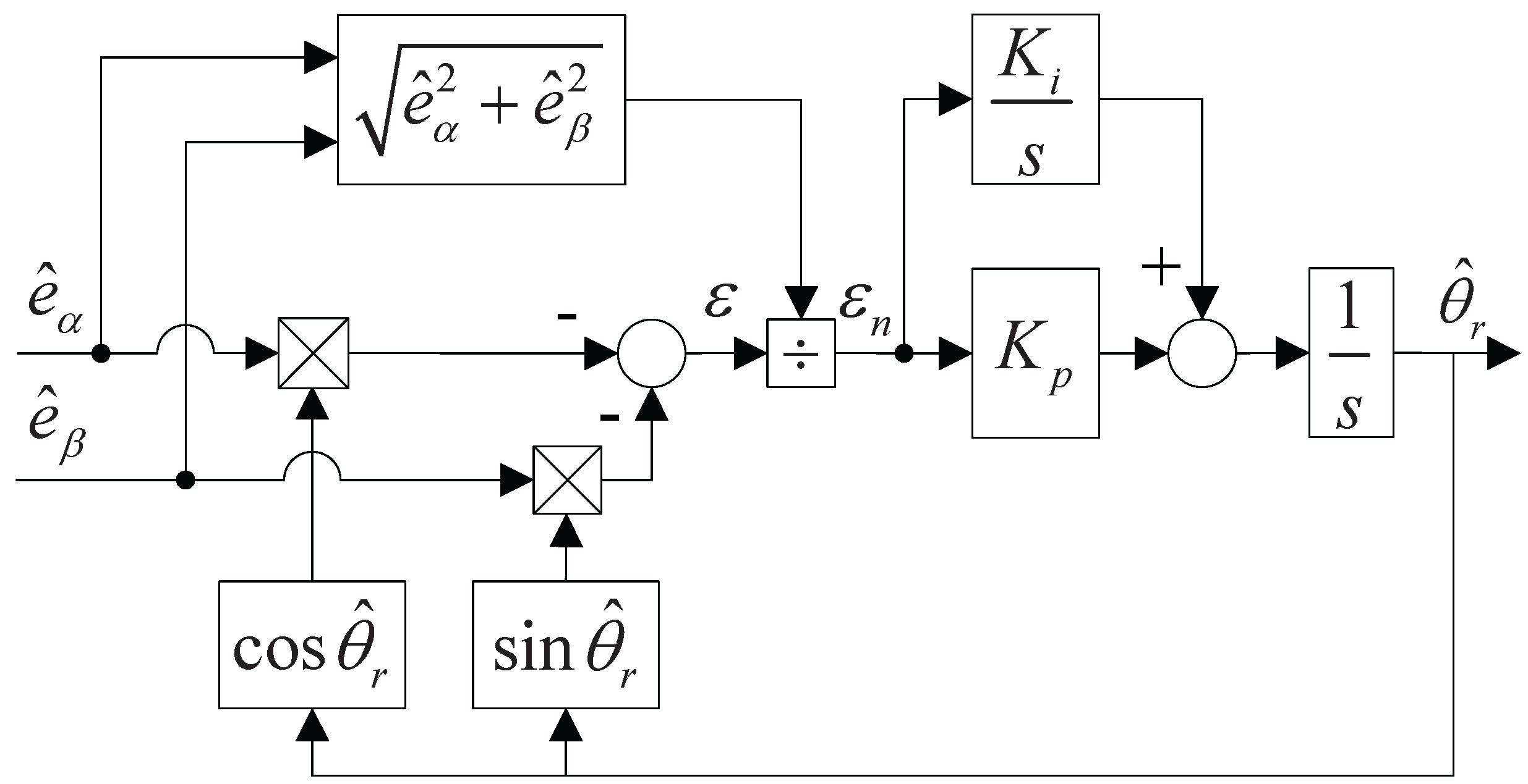
2. Sliding-Mode Observer Method for High-Speed-Range Sensorless Control

In this section, a sliding-mode observer (SMO) is adopted to estimate the rotor position at high-speed range. To utilize the SMO for an IPMSM, an extended EMF model is established in the $\alpha \beta$ frame, as shown in (1).

$$\begin{array}{cc}\hfill \left[\begin{array}{c}{u}_{\alpha }\hfill \\ u_{\beta }\hfill \end{array}\right]=& \left[\begin{array}{cc}{R}_s& {\omega }_r(L_d-L_q)\\ -{\omega }_r(L_d-L_q)& R_s\end{array}\right]\left[\begin{array}{c}{i}_{\alpha }\hfill \\ i_{\beta }\hfill \end{array}\right]+\left[\begin{array}{cc}{L}_d& 0\\ 0& L_d\end{array}\right]\frac{d}{dt}\left[\begin{array}{c}{i}_{\alpha }\hfill \\ i_{\beta }\hfill \end{array}\right]+\left[{\omega }_r{\psi }_f+\left(L_d-L_q\right)\left({\omega }_r{i}_d-{\dot{i}}_q\right)\right]\left[\begin{array}{c}-sin{\theta }_r\\ cos{\theta }_r\end{array}\right]\hfill \end{array}$$

(1)

The last term in (1) is defined as extended electromotive force (extended EMF, EEMF), $\mathit{e}$ , which is expressed as:

$$\begin{array}{cc}\hfill \mathit{e}=\left[\begin{array}{c}{e}_{\alpha }\\ e_{\beta }\end{array}\right]& =\left[{\omega }_r{\psi }_f+\left(L_d-L_q\right)\left({\omega }_r{i}_d-{\dot{i}}_q\right)\right]\left[\begin{array}{c}-sin{\theta }_r\\ cos{\theta }_r\end{array}\right]=E_{ex}\left[\begin{array}{c}-sin{\theta }_r\\ cos{\theta }_r\end{array}\right]\hfill \end{array}$$

(2)

where, $E_{ex}$ is the magnitude of $\mathit{e}$. According to (1), the current state equation for the IPMSM can be rewritten as:

$$\begin{array}{cc}\hfill \frac{d}{dt}\left[\begin{array}{c}{i}_{\alpha }\\ i_{\beta }\end{array}\right]=& \frac{1}{L_d}\left[\begin{array}{cc}-R_s& -{\omega }_r(L_d-L_q)\\ {\omega }_r(L_d-L_q)& -R_s\end{array}\right]\left[\begin{array}{c}{i}_{\alpha }\\ i_{\beta }\end{array}\right]+\frac{1}{L_d}\left[\begin{array}{c}{u}_{\alpha }\\ u_{\beta }\end{array}\right]-\frac{\mathit{e}}{L_d}\hfill \end{array}$$

(3)

Based on (3), the mathematical model of SMO can be constructed as (4).

$$\begin{array}{cc}\hfill \frac{d}{dt}\left[\begin{array}{c}{\widehat{i}}_{\alpha }\\ {\widehat{i}}_{\beta }\end{array}\right]=& \frac{1}{L_d}\left[\begin{array}{cc}-R_s& -{\omega }_r(L_d-L_q)\\ {\omega }_r(L_d-L_q)& -R_s\end{array}\right]\left[\begin{array}{c}{\widehat{i}}_{\alpha }\\ {\widehat{i}}_{\beta }\end{array}\right]+\frac{1}{L_d}\left[\begin{array}{c}{u}_{\alpha }\\ u_{\beta }\end{array}\right]-\frac{\widehat{\mathit{e}}+\mathit{z}}{L_d}\hfill \end{array}$$

(4)

where, ${[{\widehat{i}}_{\alpha },{\widehat{i}}_{\beta }]}^{\mathrm{T}}$ is the estimated current on the $\alpha$- and $\beta$-axes; $\widehat{\mathit{e}}={\left[{\widehat{e}}_{\alpha },{\widehat{e}}_{\beta }\right]}^{\mathrm{T}}$ is the estimated value of extended EMF on the $\alpha$- and $\beta$-axes. Additionally, $\mathit{z}$ is the output of the SMO control function on the $\alpha$- and $\beta$-axes, which can be expressed as:

$$\mathit{z}=\left[\begin{array}{c}{z}_{\alpha }\\ z_{\beta }\end{array}\right]=k\left[\begin{array}{c}sat({\widehat{i}}_{\alpha }-i_{\alpha })\\ sat({\widehat{i}}_{\beta }-i_{\beta })\end{array}\right]$$

(5)

where k is the SMO gain, which is calculated by Lyapunov stability analysis; $sat\left(x\right)$ is a saturation function.

Additionally, the saturation function $sat\left(x\right)$, which can be expressed as (6), is adopted in (5) as the SMO control function to suppress the chattering problem of SMO.

$$sat\left(x\right)=\left\{\begin{array}{cc}1& x\ge \delta \\ x/\delta & \left|x\right|<\delta \\ -1& x\le -\delta \end{array}\right.$$

(6)

where $\delta$ is the width of the boundary layer, which should be chosen properly. With the increase in $\delta$, the chattering problem is mitigated, however, the estimation accuracy and robustness of SMO declines. In practical application, the value of $\delta$ should be adjusted according to actual demand.

The sliding-mode surface, $\mathit{s}=0$, is defined as:

$$\mathit{s}=\left[\begin{array}{c}{\tilde{i}}_{\alpha }\\ {\tilde{i}}_{\beta }\end{array}\right]=\left[\begin{array}{c}{\widehat{i}}_{\alpha }-i_{\alpha }\\ {\widehat{i}}_{\beta }-i_{\beta }\end{array}\right]=0$$

(7)

By subtracting (3) from (4), the dynamic motion equation of SMO is expressed as:

$$\dot{\mathit{s}}=\frac{1}{L_d}\left[\begin{array}{cc}-R_s& -{\omega }_r(L_d-L_q)\\ {\omega }_r(L_d-L_q)& -R_s\end{array}\right]·\mathit{s}-\frac{\widehat{\mathit{e}}+\mathit{z}-\mathit{e}}{L_d}$$

(8)

When the system converges to sliding-mode state, it maintains that:

$$\dot{\mathit{s}}=\mathit{s}=0$$

(9)

Then, by substituting (9) into (8), it can be obtained that:

$$\widehat{\mathit{e}}+\mathit{z}=\mathit{e}$$

(10)

In (10), the phase angle of the extended EMF $\mathit{e}$ just contains the information of rotor position ${\theta }_r$, and the frequency of $\mathit{e}$ is rotor speed ${\omega }_r$. In addition, the $\widehat{\mathit{e}}$ is obtained by filtering the SMO control output $\mathit{z}$ with a low-pass filter (LPF). The LPF should be properly designed so that the phase lag between $\widehat{\mathit{e}}$ and $\mathit{z}$ at frequency ${\omega }_r$ can be neglected. In this case, the phase angles of $\widehat{\mathit{e}}$ and $\mathit{z}$ at frequency ${\omega }_r$ are both equal to the phase angle of $\mathit{e}$. Then, the $\widehat{\mathit{e}}$ can be utilized to estimate rotor position. The diagram of the rotor position estimation based on the SMO method is shown in Figure 1.

When using the normal LPF to filter the $\mathit{z}$, the phase lag of $\widehat{\mathit{e}}$ should be well-compensated. However, with the variation of rotor speed ${\omega }_r$, the calculation of phase lag is difficult. Therefore, an adaptive LPF is adopted, as shown in Figure 1.

A first-order LPF is utilized inside the adaptive LPF, whose cut-off frequency is set as the estimated rotor speed ${\widehat{\omega }}_r$. In steady state, when ${\widehat{\omega }}_r={\omega }_r$, the phase lag caused by the LPF is always a constant value $\pi /4$ at any rotor speed. After compensating the phase lag $\pi /4$, the $\widehat{\mathit{e}}$ can be utilized to estimate rotor position.

Normally, the rotor position can be estimated by using the arc-tangent function (11) directly.

$${\widehat{\mathrm{\theta }}}_r=-{tan}^{-1}({\widehat{e}}_{\alpha }/{\widehat{e}}_{\beta })$$

(11)

However, due to the chattering problem of SMO, the rotor position calculated directly by the arc-tangent function will be seriously disturbed. In addition, since (11) contains division, it will produce huge estimation error when the ${\widehat{e}}_{\beta }$ crosses zero. Therefore, a phase-locked loop (PLL) algorithm is utilized to estimate the rotor position, as shown in Figure 2.

In Figure 2, after the normalization, the equivalent position error signal ${\epsilon }_n$ can be expressed as:

$$\begin{array}{cc}\hfill {\epsilon }_n& =\frac{1}{\sqrt{{\widehat{e}}_{\alpha }^2+{\widehat{e}}_{\beta }^2}}[-{\widehat{e}}_{\alpha }cos{\widehat{\theta }}_r-{\widehat{e}}_{\beta }sin{\widehat{\theta }}_r]\hfill \\ \hfill & =\frac{1}{E_{ex}}[E_{ex}sin{\theta }_{r}cos{\widehat{\theta }}_r-E_{ex}cos{\theta }_{r}sin{\widehat{\theta }}_r]\hfill \\ \hfill & =sin({\theta }_r-{\widehat{\theta }}_r)\approx {\theta }_r-{\widehat{\theta }}_r\hfill \end{array}$$

(12)

Then, the closed-loop transfer function of PLL $G_{PLL}\left(s\right)$ can be expressed as:

$$G_{PLL}\left(s\right)=\frac{{\widehat{\theta }}_r}{{\theta }_r}=\frac{K_{p}s+K_i}{s^2+K_{p}s+K_i}$$

(13)

The $G_{PLL}\left(s\right)$ is a second-order transfer function. By using the pole placement method, the parameters $K_p$ and $K_i$ can be easily designed.

To guarantee the convergence of SMO, the SMO gain k should be chosen according to the Lyapunov stability analysis. Choosing a positive definite Lyapunov function as:

$$V=\frac{1}{2}{\mathit{s}}^T\mathit{s}=\frac{1}{2}({\tilde{i}}_{\alpha }^2+{\tilde{i}}_{\beta }^2)$$

(14)

According to the Lyapunov stability theorem, $\dot{V}$ should be negative definite, namely $\dot{V}<0$. The derivative of (14) can be expressed as:

$$\begin{array}{cc}\hfill \dot{V}& ={\mathit{s}}^T\dot{\mathit{s}}\hfill \\ \hfill & ={\tilde{i}}_{\alpha }·{\dot{\tilde{}}i}_{\alpha }+{\tilde{i}}_{\beta }·{\dot{\tilde{}}i}_{\beta }\hfill \\ \hfill & ={\tilde{i}}_{\alpha }\left\{-\frac{R_s}{L_d}{\tilde{i}}_{\alpha }-\frac{L_d-L_q}{L_d}{\widehat{\omega }}_e{\tilde{i}}_{\beta }-\frac{1}{L_d}{\tilde{e}}_{\alpha }-\frac{1}{L_d}k\mathrm{sat}\left({\tilde{i}}_{\alpha }\right)\right\}+{\tilde{i}}_{\beta }\left\{-\frac{R_s}{L_d}{\tilde{i}}_{\beta }+\frac{L_d-L_q}{L_d}{\widehat{\omega }}_e{\tilde{i}}_{\alpha }-\frac{1}{L_d}{\tilde{e}}_{\beta }-\frac{1}{L_d}k\mathrm{sat}\left({\tilde{i}}_{\beta }\right)\right\}\hfill \\ \hfill & =-\frac{R_s}{L_d}\left({\tilde{i}}_{\alpha }^2+{\tilde{i}}_{\beta }^2\right)-\frac{1}{L_d}\left\{{\tilde{i}}_{\alpha }\left({\tilde{e}}_{\alpha }+k\mathrm{sat}\left({\tilde{i}}_{\alpha }\right)\right)\right\}-\frac{1}{L_d}\left\{{\tilde{i}}_{\beta }\left({\tilde{e}}_{\beta }+k\mathrm{sat}\left({\tilde{i}}_{\beta }\right)\right)\right\}\hfill \\ \hfill & =V_1-V_2\hfill \end{array}$$

(15)

where,

$$V_1=-\frac{R_s}{L_d}\left({\tilde{i}}_{\alpha }^2+{\tilde{i}}_{\beta }^2\right)$$

(16)

$$\begin{array}{cc}\hfill V_2& =\frac{1}{L_d}\left\{{\tilde{i}}_{\alpha }\left({\tilde{e}}_{\alpha }+k\mathrm{sat}\left({\tilde{i}}_{\alpha }\right)\right)\right\}+\frac{1}{L_d}\left\{{\tilde{i}}_{\beta }\left({\tilde{e}}_{\beta }+k\mathrm{sat}\left({\tilde{i}}_{\beta }\right)\right)\right\}\hfill \\ \hfill & =\frac{1}{L_d}\left\{{\tilde{i}}_{\alpha }\left(\frac{s+2{\omega }_c}{s+{\omega }_c}k\mathrm{sat}\left({\tilde{i}}_{\alpha }\right)-e_{\alpha }\right)+{\tilde{i}}_{\beta }\left(\frac{s+2{\omega }_c}{s+{\omega }_c}k\mathrm{sat}\left({\tilde{i}}_{\beta }\right)-e_{\beta }\right)\right\}\hfill \end{array}$$

(17)

As shown in (16), $V_1$ is a constant negative. Since the cutoff frequency of the low-pass filter ${\omega }_c$ is relatively large, then $\frac{s+2{\omega }_c}{s+{\omega }_c}\approx 2$. If k is large enough, in which:

$$k>\frac{1}{2}max\left(\left|{\mathrm{e}}_{\alpha }\right|,\left|e_{\beta }\right|\right)$$

(18)

then the SMO method can be converged. When V is attenuated to 0, ${\tilde{i}}_{\alpha }$, and ${\tilde{e}}_{\alpha }$ are equal to 0, then the estimated currents are converged to the actual value.

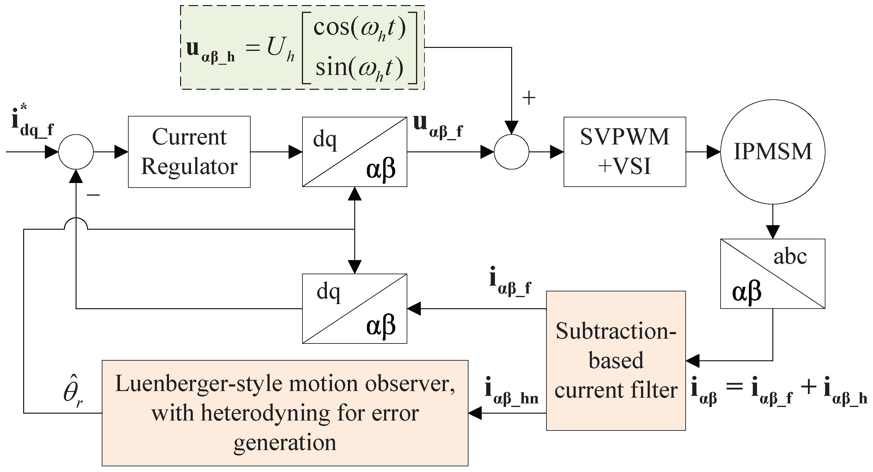
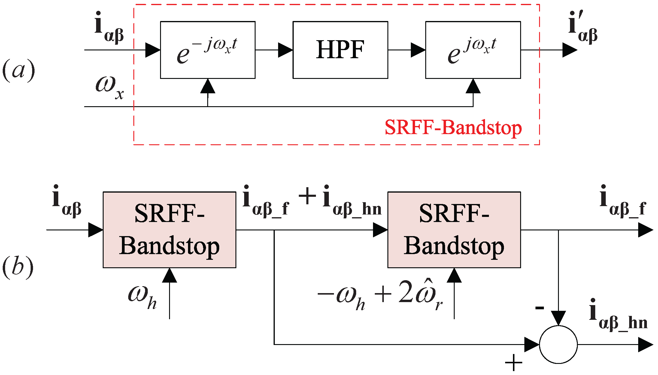
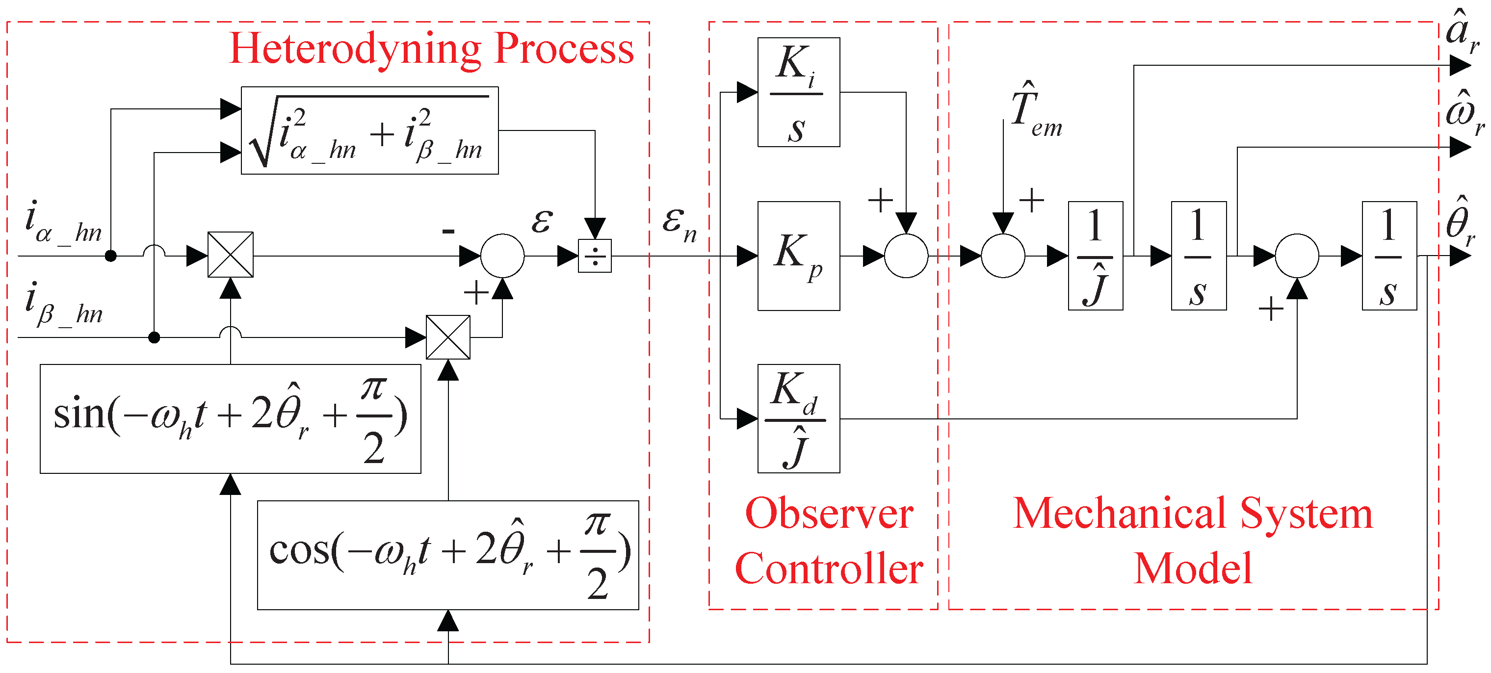
3. Rotating Voltage High-Frequency Injection Method for Low-Speed-Range Sensorless Control

To analyze the principle of the rotating voltage HFI-based sensorless method, the mathematical model of an IPMSM under high-frequency excitation is established in the following. The flux model of the IPMSM in the $dq$ frame is rewritten as:

$$\left[\begin{array}{c}{\psi }_d\\ {\psi }_q\end{array}\right]=\left[\begin{array}{cc}{L}_d& 0\\ 0& L_q\end{array}\right]\left[\begin{array}{c}{i}_d\\ i_q\end{array}\right]+\left[\begin{array}{c}{\psi }_f\\ 0\end{array}\right]$$

(19)

By using coordinate transformation with (19), the flux model in the $\alpha \beta$ frame can be expressed as:

$${\mathbf{\psi }}_{\mathbf{\alpha }\mathbf{\beta }}={\mathit{L}}_{\mathbf{\alpha }\mathbf{\beta }}·{\mathit{i}}_{\mathbf{\alpha }\mathbf{\beta }}+{\psi }_f{e}^{j{\theta }_r}$$

(20)

where

$$\begin{array}{c}{\mathit{L}}_{\mathbf{\alpha }\mathbf{\beta }}=\left[\begin{array}{cc}\sum L-\Delta Lcos\left(2{\theta }_r\right)& -\Delta Lsin\left(2{\theta }_r\right)\\ -\Delta Lsin\left(2{\theta }_r\right)& \sum L+\Delta Lcos\left(2{\theta }_r\right)\end{array}\right]\\ \sum L=\frac{L_q+L_d}{2}\Delta L=\frac{L_q-L_d}{2}\\ {\mathbf{\psi }}_{\mathbf{\alpha }\mathbf{\beta }}={\left[{\psi }_{\alpha },{\psi }_{\beta }\right]}^T{\mathit{i}}_{\mathbf{\alpha }\mathbf{\beta }}={\left[i_{\alpha },i_{\beta }\right]}^T\end{array}$$

Then, according to (20), the voltage equation in the $\alpha \beta$ frame can be expressed as:

$$\begin{array}{cc}\hfill {\mathit{u}}_{\mathbf{\alpha }\mathbf{\beta }}& =R_s·{\mathit{i}}_{\mathbf{\alpha }\mathbf{\beta }}+\frac{d}{dt}{\mathbf{\psi }}_{\mathbf{\alpha }\mathbf{\beta }}\hfill \\ \hfill & =R_s·{\mathit{i}}_{\mathbf{\alpha }\mathbf{\beta }}+\frac{d}{dt}({\mathit{L}}_{\mathbf{\alpha }\mathbf{\beta }}·{\mathit{i}}_{\mathbf{\alpha }\mathbf{\beta }})+j{\omega }_r{\psi }_f{e}^{j{\theta }_r}\hfill \end{array}$$

(21)

For the rotating voltage HFI sensorless method, a rotating voltage signal is injected into the $\alpha \beta$ frame, which can be expressed as:

$${\mathit{u}}_{\mathbf{\alpha }\mathbf{\beta }\_\mathit{h}}=U_h·e^{j{\omega }_{h}t}=U_h\left[\begin{array}{c}cos\left({\omega }_{h}t\right)\\ sin\left({\omega }_{h}t\right)\end{array}\right]$$

(22)

where, $U_h$ and ${\omega }_h$ are the amplitude and angular frequency of the injected high-frequency voltage signal, respectively.

When the high-frequency voltage ${\mathit{u}}_{\mathbf{\alpha }\mathbf{\beta }\_\mathbf{h}}$ is injected, two simplifications can be made in the IPMSM voltage Equation (21). First, since the reactance part is dominating the machine impedance under high-frequency voltage source, the term of the voltage drop on resistance $R_s·{\mathit{i}}_{\mathbf{\alpha }\mathbf{\beta }}$ in (21) can be neglected. Second, since the HFI method is utilized in low-speed range, where the rotor speed ${\omega }_r$ can be considered much lower than the frequency of high-frequency voltage ${\omega }_h$, then the third term $j{\omega }_r{\psi }_f{e}^{j{\theta }_r}$ in (21) can be neglected.

Then, after substituting (22) into (21) and simplifying the two terms described above, the voltage Equation (21) can be written as:

$${\mathit{u}}_{\mathbf{\alpha }\mathbf{\beta }\_\mathit{h}}=\frac{d}{dt}({\mathit{L}}_{\mathbf{\alpha }\mathbf{\beta }}·{\mathit{i}}_{\mathbf{\alpha }\mathbf{\beta }\_\mathit{h}})$$

(23)

By solving (23), the high-frequency current response can be obtained as (24).

$$\begin{array}{cc}\hfill {\mathit{i}}_{\mathbf{\alpha }\mathbf{\beta }\_\mathit{h}}& ={\mathit{L}}_{\mathbf{\alpha }\mathbf{\beta }}^{-\mathbf{1}}·\left(\frac{1}{j{\omega }_h}{\mathit{u}}_{\mathbf{\alpha }\mathbf{\beta }}\right)\hfill \\ \hfill & =I_p·e^{j({\omega }_{h}t-\pi /2)}+I_n·e^{j(-{\omega }_{h}t+2{\theta }_r+\pi /2)}\hfill \end{array}$$

(24)

where

$$\begin{array}{c}{I}_p=\frac{U_h}{{\omega }_h}·\frac{\sum L}{\sum L^2-\Delta L^2}{I}_n=\frac{U_h}{{\omega }_h}·\frac{\Delta L}{\sum L^2-\Delta L^2}\end{array}$$

$I_p$ and $I_n$ are the amplitude of the positive- and negative-sequence currents, respectively. $\Delta L$ and $\sum L$ are the difference and average inductances. In Equation (24), the first term, which is called the positive-sequence current component, is a current vector rotating at the frequency ${\omega }_h$. The second term, which is called the negative-sequence current component, is a current vector rotating at the frequency $-{\omega }_h+2{\omega }_r$. Among them, the information of rotor position is contained in the second term.

Therefore, the rotor position can be estimated through extracting and analyzing the negative-sequence current from the measured current. The schemetic diagram of rotor position identification is shown in Figure 3.

By using a subtraction-based current filter on the total current response ${\mathit{i}}_{\mathbf{\alpha }\mathbf{\beta }}$, the negative-sequence carrier current ${\mathit{i}}_{\mathbf{\alpha }\mathbf{\beta }\_\mathbf{hn}}$ and fundamental current ${\mathit{i}}_{\mathbf{\alpha }\mathbf{\beta }\_\mathit{f}}$ are separated. Then, the Luenberger-style motion observer is utilized to analyze the ${\mathit{i}}_{\mathbf{\alpha }\mathbf{\beta }\_\mathit{hn}}$ to identify the rotor position, and the ${\mathit{i}}_{\mathbf{\alpha }\mathbf{\beta }\_\mathit{f}}$ is utilized to feed back to the current regulator. Figure 4 and Figure 5 show the diagrams of subtraction-based current filter and Luenberger-style motion observer, respectively.

The rotating-voltage-based HFI method showed excellent performance when using the synchronous reference frame filter (SRFF) to isolate the ${\mathit{i}}_{\mathbf{\alpha }\mathbf{\beta }\_\mathit{hn}}$ and ${\mathit{i}}_{\mathbf{\alpha }\mathbf{\beta }\_\mathit{f}}$ [1,34]. Figure 4a shows the diagram of the bandstop SRFF. In Figure 4a, the input signal ${\mathit{i}}_{\mathbf{\alpha }\mathbf{\beta }}$ is first transformed into a reference frame rotating with the desired frequency ${\omega }_x$. Then, the signal component which has the frequency of ${\omega }_x$ at the original stationary frame is now transformed to a DC signal at this rotating frame. In this case, this signal component can be eliminate by a simple high-pass filter (HPF). After that, the remaining signal components are transformed to the original stationary frame. In this bandstop SRFF, only a simple first-order filter can guarantee nearly zero magnitude gain at the desired bandstop frequency ${\omega }_x$. Additionally, at other frequencies, the distortions of both magnitude and phase are minimized. The transfer function of this bandstop SRFF is given in (25).

$$\frac{{{\mathit{i}}^{\prime }}_{\mathbf{\alpha }\mathbf{\beta }}}{{\mathit{i}}_{\mathbf{\alpha }\mathbf{\beta }}}=\frac{s-j·{\omega }_x}{s+{\omega }_b-j·{\omega }_x}$$

(25)

where ${\omega }_x$ is the frequency of the current component which needs to be eliminated, and ${\omega }_b$ is the bandwidth of the HPF inside the bandstop SRFF, then the bandwidth of bandstop SRFF is $({\omega }_x-{\omega }_b,{\omega }_x+{\omega }_b)$.

The structure of the subtraction-based current filter is shown in Figure 4b [35], which is set up based on the bandstop SRFF to extract the fundamental ${\mathit{i}}_{\mathbf{\alpha }\mathbf{\beta }\_\mathit{f}}$ and the negative sequence ${\mathit{i}}_{\mathbf{\alpha }\mathbf{\beta }\_\mathit{hn}}$ from the measured ${\mathit{i}}_{\mathbf{\alpha }\mathbf{\beta }}$. First, a bandstop SRFF with the bandstop frequency of ${\omega }_h$ is utilized to eliminate the positive sequence current ${\mathit{i}}_{\mathbf{\alpha }\mathbf{\beta }\_\mathit{hp}}$ from the total current ${\mathit{i}}_{\mathbf{\alpha }\mathbf{\beta }}$. Then, a second bandstop SRFF with the bandstop frequency of $-{\omega }_h+2{\widehat{\omega }}_r$ is used to remove the signal ${\mathit{i}}_{\mathbf{\alpha }\mathbf{\beta }\_\mathit{hn}}$ from the remaining signal. With these two bandstop SRFFs, the output signal is mainly ${\mathit{i}}_{\mathbf{\alpha }\mathbf{\beta }\_\mathit{f}}$. Additionally, ${\mathit{i}}_{\mathbf{\alpha }\mathbf{\beta }\_\mathit{hn}}$ can be extracted by subtracting this ${\mathit{i}}_{\mathbf{\alpha }\mathbf{\beta }\_\mathit{f}}$ from the output of the first bandstop SRFF.

Then, a Luenberger-style motion observer [36] is utilized to estimate the electrical rotor position by analyzing the ${\mathit{i}}_{\mathbf{\alpha }\mathbf{\beta }\_\mathit{hn}}$, and its diagram is shown in Figure 5.

In Figure 5, the position estimation error ${\epsilon }_n$ is calculated by a heterodyning process, which can be considered as the result of the vector cross-product, as shown in (26).

$$\begin{array}{cc}\hfill {\epsilon }_n& =\frac{1}{\sqrt{i_{\alpha \_hn}^2+i_{\beta \_hn}^2}}·e^{j(-{\omega }_{h}t+2{\widehat{\theta }}_r+\frac{\pi }{2})}\times {\mathit{i}}_{\mathbf{\alpha }\mathbf{\beta }\_\mathit{hn}}\hfill \\ \hfill & =\frac{1}{I_{hn}}·e^{j(-{\omega }_{h}t+2{\widehat{\theta }}_r+\frac{\pi }{2})}\times I_{hn}{e}^{j(-{\omega }_{h}t+2{\theta }_r+\frac{\pi }{2})}\hfill \\ \hfill & =sin\left(2({\theta }_r-{\widehat{\theta }}_r)\right)\approx 2\Delta {\widehat{\theta }}_r\hfill \end{array}$$

(26)

According to (26), the $sin\left(2({\theta }_r-{\widehat{\theta }}_r)\right)$ can be considered equal to $2\Delta {\widehat{\theta }}_r$ when the difference between ${\theta }_r$ and ${\widehat{\theta }}_r$ is small enough. However, because of the existence of coefficient 2, the calculation results of ${\epsilon }_n$ are the same when the estimated position is either ${\widehat{\theta }}_r$ or ${\widehat{\theta }}_r+\pi$. Therefore, the rotor magnetic poles N and S cannot be distinguished when using the HFI method described above. Hence, before motor start-up, an extra rotor polarity detection program should be implemented.

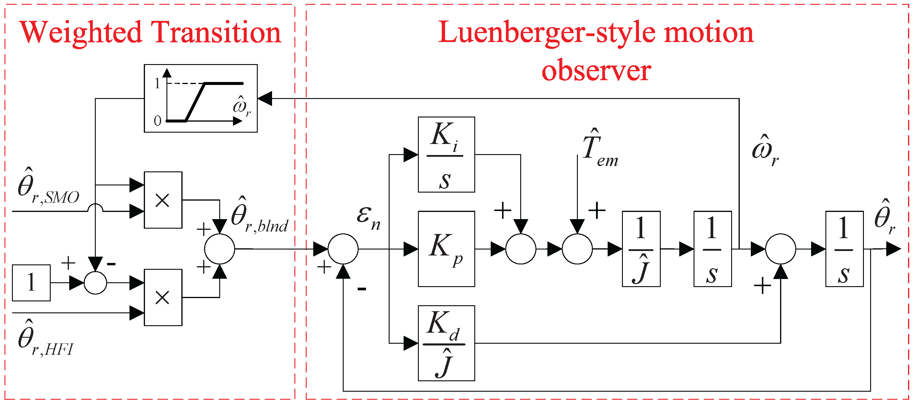
4. Transition between the High-Speed and Low-Speed Sensorless Control

As described above, the SMO-based method only provides reliable estimated rotor position in medium- and high-speed ranges, but it fails in low-speed range. On the other hand, the HFI-based method can provide accurate estimated rotor position at standstill and low-speed range, but it fails in high-speed range. Therefore, in order to combine these two methods and achieve sensorless control in the whole speed range, a suitable transition algorithm between these two methods should be implemented. The diagram of the transition algorithm adopted in this paper is shown in Figure 6.

In Figure 6, a speed-dependent weighted function is utilized to blend the two rotor positions ${\widehat{\theta }}_{r,SMO}$ and ${\widehat{\theta }}_{r,HFI}$, which are estimated by the SMO method and HFI method, respectively. Then, the blended position estimation ${\widehat{\theta }}_{r,blnd}$ is filtered by a Luenberger-style motion observer. The output of Luenberger-style motion observer ${\widehat{\theta }}_r$ is just the desired estimated rotor position. Additionally, the estimated speed ${\widehat{\omega }}_r$ is regarded as the indicator of the weighted function.

Then, the speed-dependent weighted function can be expressed as:

$${\widehat{\theta }}_{r,blnd}=g_w{\widehat{\theta }}_{r,SMO}+(1-g_w){\widehat{\theta }}_{r,HFI}$$

(27)

$$g_w=\left\{\begin{array}{cc}1,& \left|{\widehat{\omega }}_r\right|\ge {\omega }_{upper}\\ \frac{\left|{\widehat{\omega }}_r\right|-{\omega }_{lower}}{{\omega }_{upper}-{\omega }_{lower}}& {\omega }_{lower}<\left|{\widehat{\omega }}_r\right|<{\omega }_{upper}\\ 0& \left|{\widehat{\omega }}_r\right|\le {\omega }_{lower}\end{array}\right.$$

(28)

where $g_w$ is the weight coefficient; ${\omega }_{lower}$ and ${\omega }_{upper}$ are the lower and upper speed thresholds of the transition region, respectively, which can be chosen as about 10% and 20% of the rated speed.

5. Experimental Results

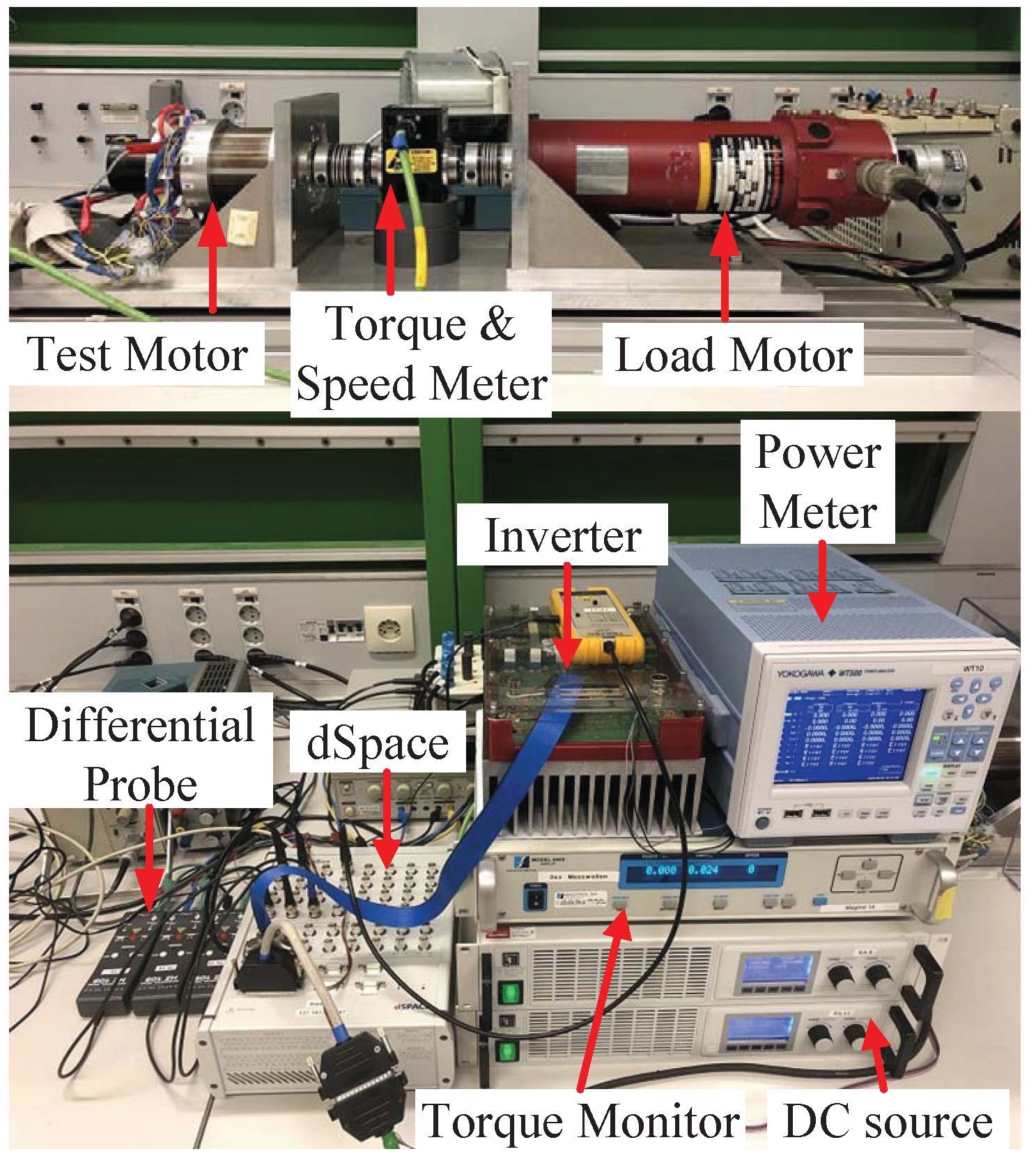
5.1. Test Bench Introduction

The test bench utilized in the experiments of this paper is shown in Figure 7.

The test motor studied in this paper is a concentrated windings IPMSM, the parameters of which are shown in

Table 1. Parameters of the IPMSM.

Rated torque (N·m )	2
Rated current (Arms)/voltage (Vrms)	40/13
Number of pole pairs	5
$dq$-axis inductance (mH)	0.065/0.09
Resistance (m$\mathrm{\Omega }$)	36
PM flux linkage (Vs)	0.007
Rated speed (rpm)	2000
Moment of inertia (g$·{\mathrm{m}}^2$)	1.87

. As for the control system, the dSpace MicroLabBox is employed as controller. The inverter is based on MOSFET IPB180N10S4-02. In this section, the switching frequency is set as 10 kHz, and the dead time is 1 us. To verify the accuracy of rotor position estimation, an absolute encoder (ROC410) with 10-bit resolution is mounted on the rotor. The load motor is a DC motor, which is controlled by SIEMENS DC Converter.

5.2. Position Estimation Based on SMO Method for High-Speed Range

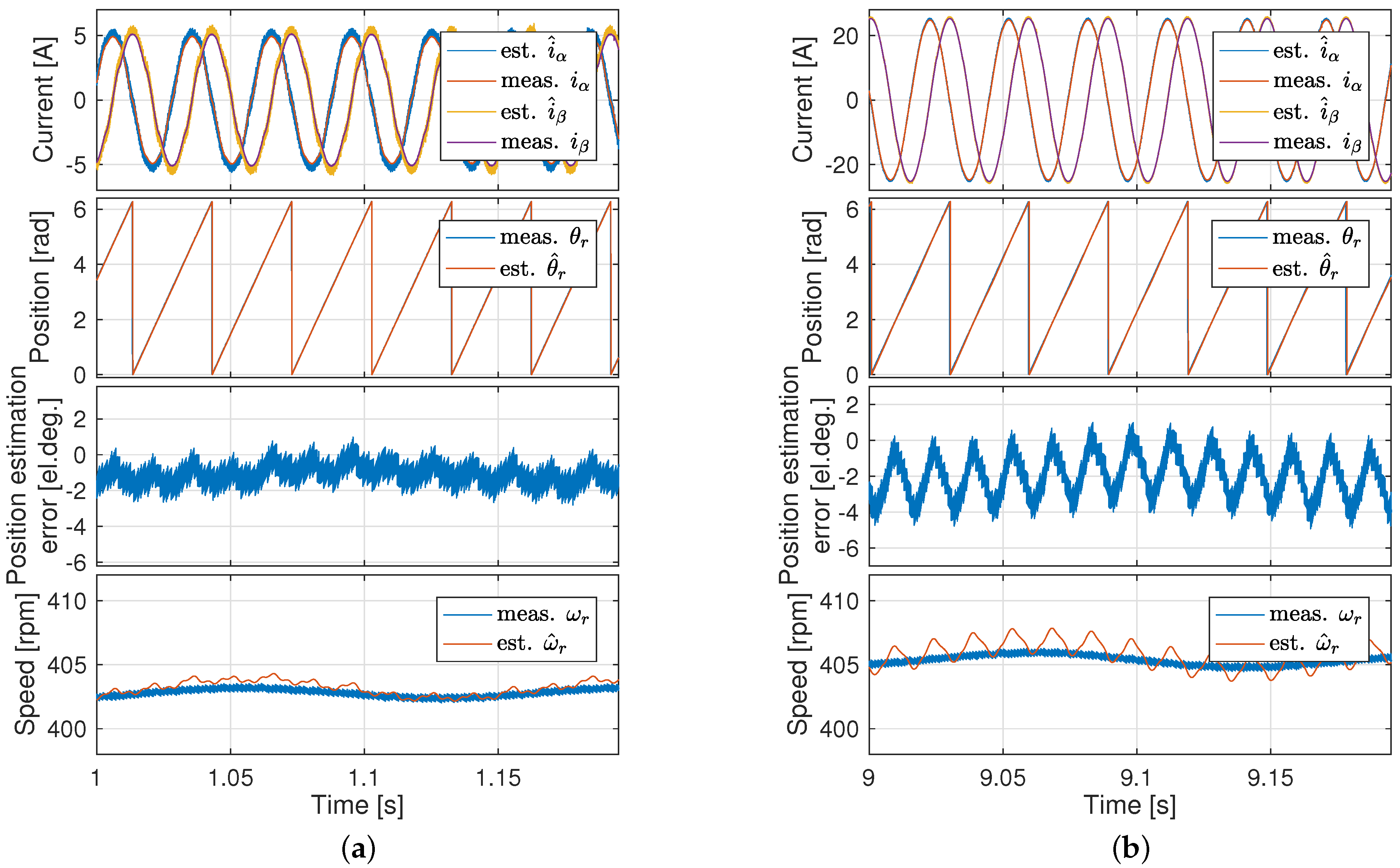
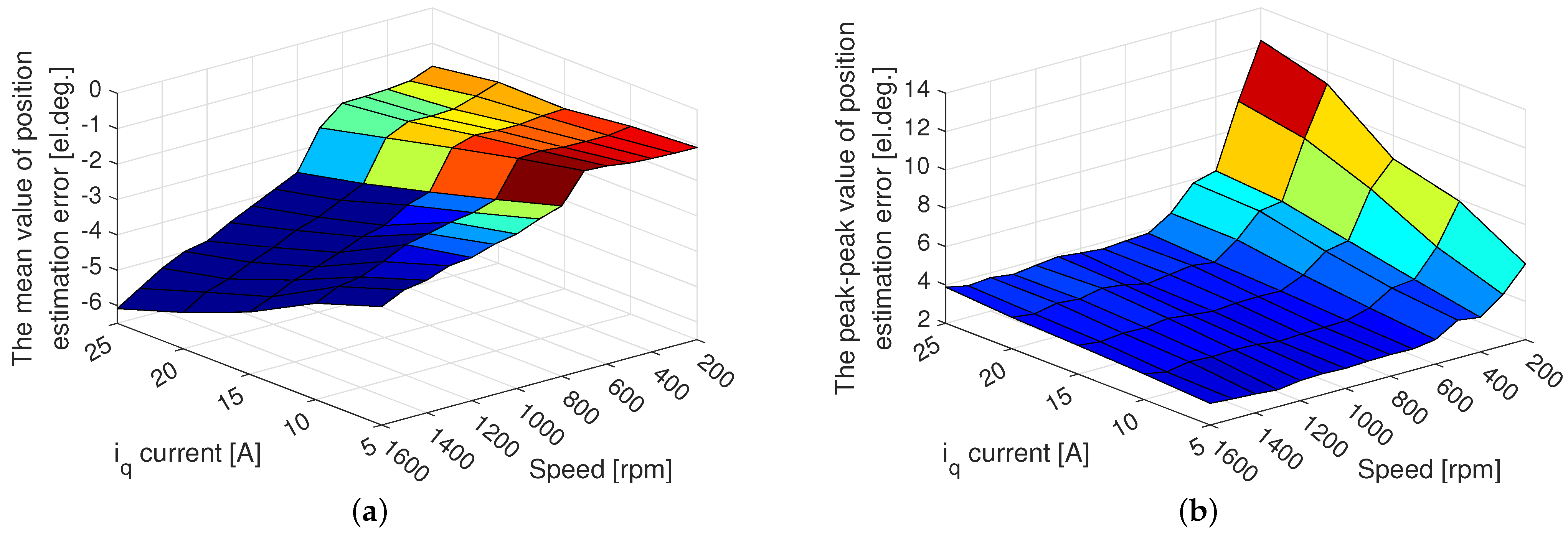
5.2.1. Steady-State Experiments of Sensorless Control Based on SMO Method

In order to evaluate the steady-state performance of the position estimation based on the SMO method, the experiments are conducted at the operating points $(400\mathrm{rpm},5\mathrm{A})$ and $(400\mathrm{rpm},25\mathrm{A})$. The corresponding experimental results are shown in Figure 8a,b, respectively.

In Figure 8a,b, the estimated angles in both two operating points show high accuracy. Their position estimation errors are both less than $5\text{el.deg.}$ However, with the increase in load current, the ripples of the position estimation error in Figure 8b become much larger than the ripples of the position estimation error in Figure 8a.

To further investigate the steady-state performance of this SMO-based position estimation method, the same experiments are conducted at different speeds and load currents, and the results of the position estimation errors are summarized in Figure 9.

Figure 9a shows the mean value of the position estimation error, and Figure 9b shows the peak–peak value of the position estimation error. From Figure 9a, the mean errors of the SMO-based position estimation are all less than 6 $\text{el.deg.}$ when the speed is between 200 $\mathrm{rpm}$ to 1600 $\mathrm{rpm}$ and the current is between 5 $\mathrm{A}$ to 25 $\mathrm{A}$. With the increase in speed and load current, the mean error of position estimation only increases a little. From Figure 9b, it is shown that the peak–peak error of the position estimation increases with the decrease in speed and the increase in load current. However, when the speed is higher than 600 $\mathrm{rpm}$, the impact of load current on the peak–peak error of the position estimation becomes much smaller.

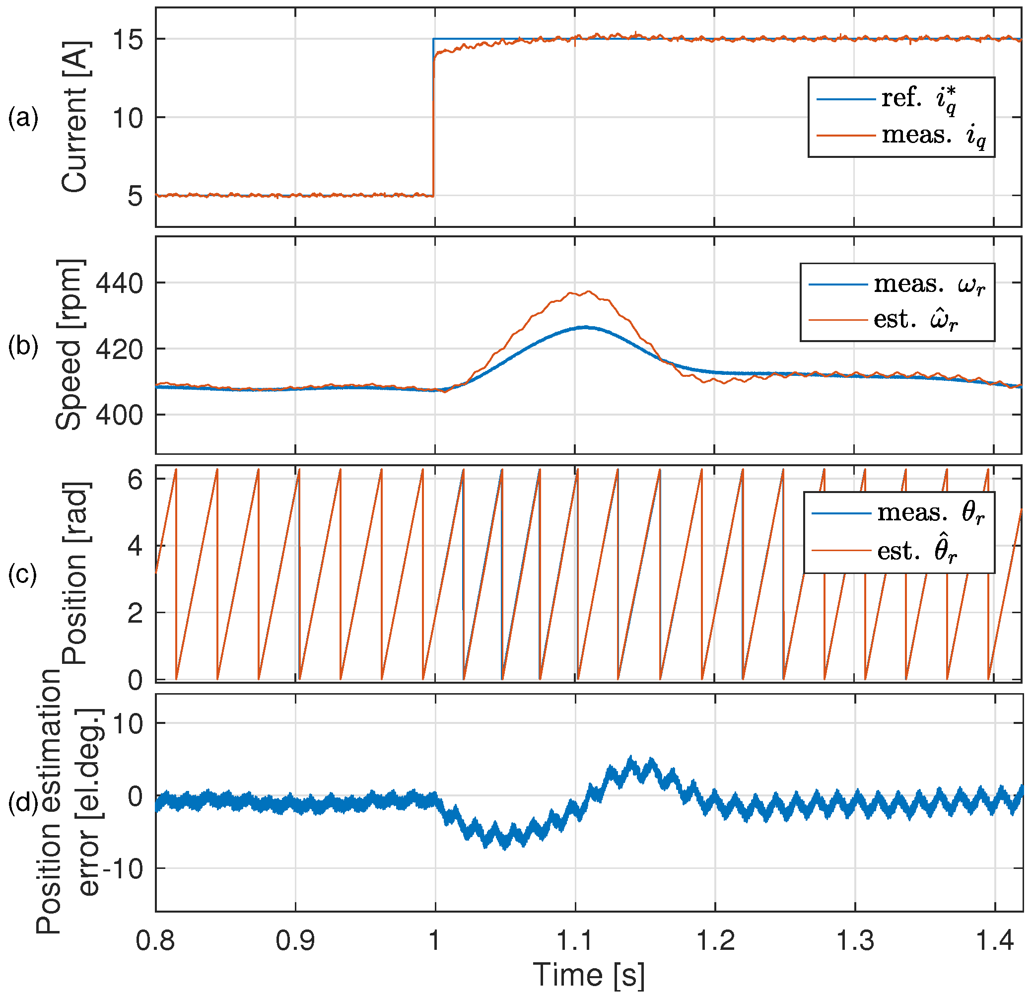
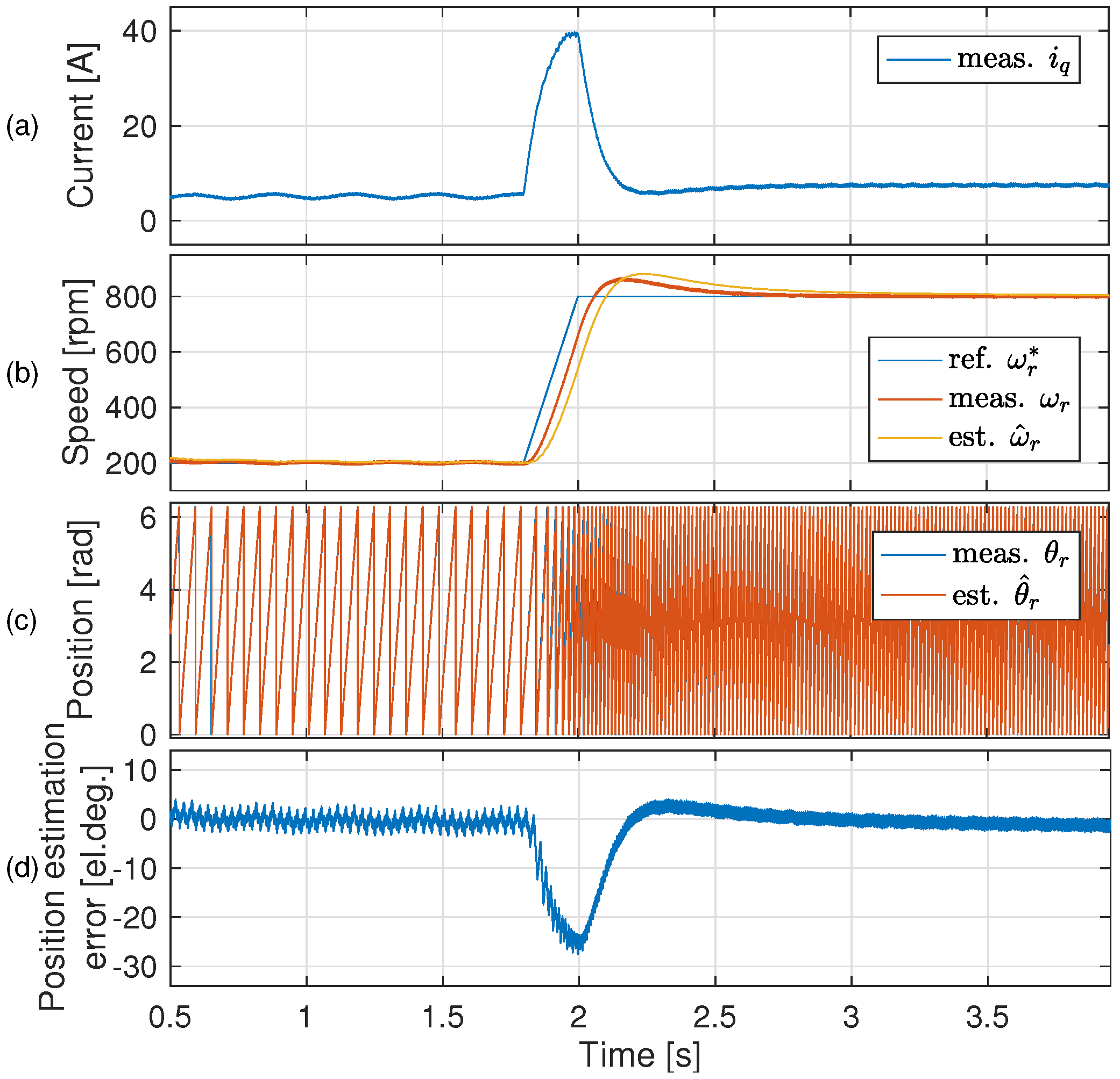
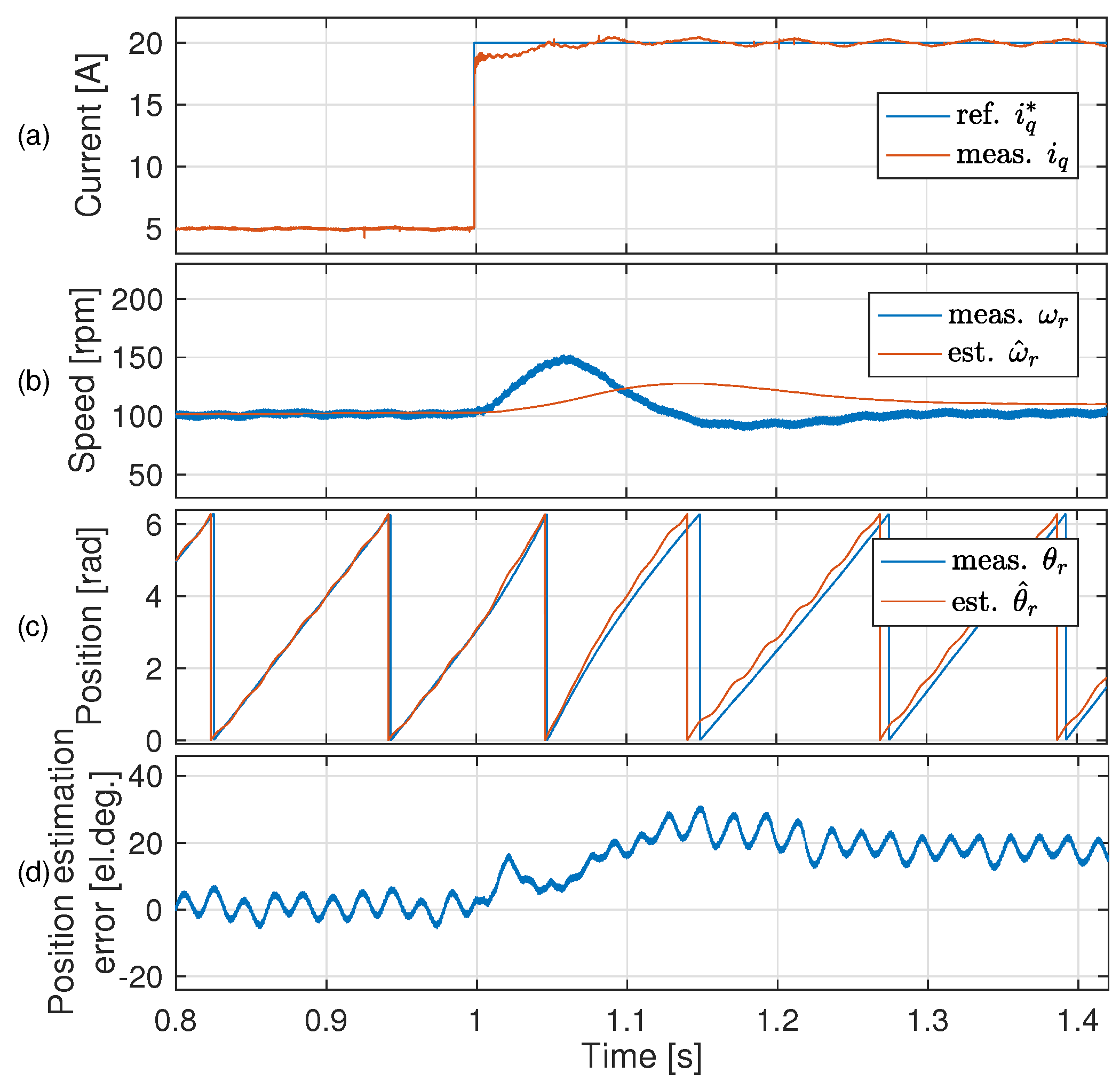
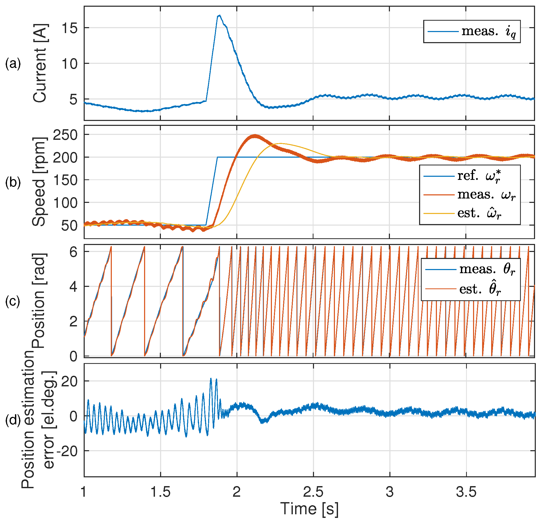
5.2.2. Dynamic Experiments of Sensorless Control Based on SMO Method

In order to evaluate the dynamic performance of the SMO-based position estimation, the current step test and speed acceleration test are implemented, and their experimental results are shown in Figure 10 and Figure 11, respectively.

Referring to the current step test, the tested IPMSM works under current control, and the load motor operates under speed control. At 1.0 $\mathrm{s}$, a step current command $i_q^{*}$ from 5 $\mathrm{A}$ to 15 $\mathrm{A}$ is set to the tested IPMSM, while the rotor speed is maintained at 400 $\mathrm{rpm}$ by the load motor. From Figure 10a, the current feedback tracks the current step command very well. During the dynamic process, the position estimation error is smaller than 5 $\text{el.deg.}$

In the speed acceleration test, the tested IPMSM operates under speed control, and the load motor runs under current control. At 1.8 $\mathrm{s}$, a ramp speed command ${\omega }_r^{*}$ from 200 $\mathrm{rpm}$ to 800 $\mathrm{rpm}$ is set to the tested IPMSM, while the load motor provides a constant load torque of 0.1 $\text{N.m.}$. In Figure 11d, during the acceleration process, the position estimation error is smaller than 25 $\text{el.deg.}$

5.3. Position Estimation Based on HFI Method for Low-Speed Range

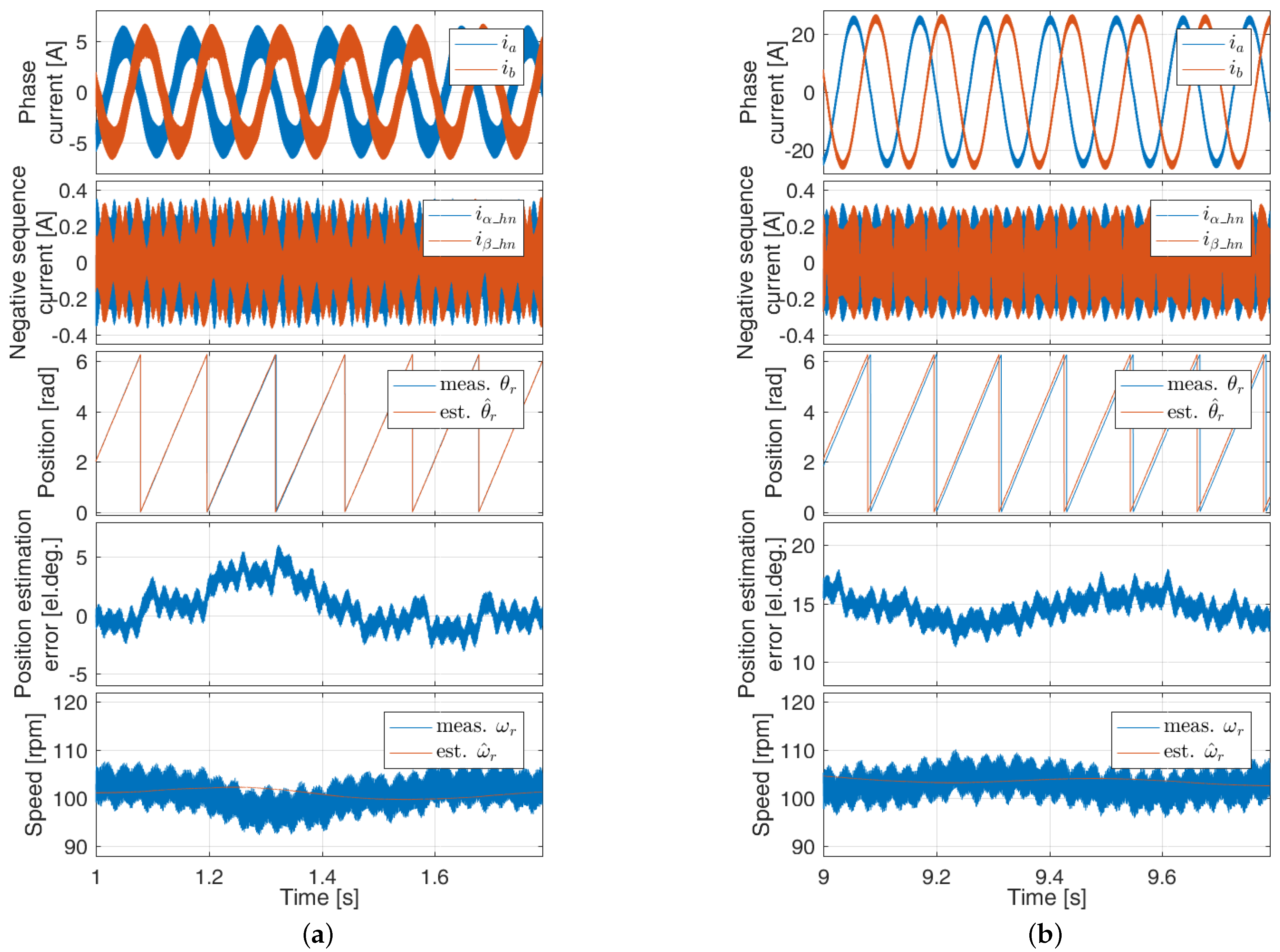
5.3.1. Steady-State Experiments of Sensorless Control Based on HFI Method

In order to evaluate the steady-state performance of the position estimation based on the HFI method, the experiments are carried out at the steady operating points $(100\mathrm{rpm},5\mathrm{A})$ and $(100\mathrm{rpm},25\mathrm{A})$. The corresponding experimental results are shown in Figure 12a,b, respectively.

In Figure 12a, the estimated rotor position shows high accuracy with the current of 5 $\mathrm{A}$. Its position estimation error is less than 5 $\text{el.deg.}$ However, in Figure 12b, when the current load is increased to 25 $\mathrm{A}$, the position estimation error becomes about 15 $\text{el.deg.}$

To further investigate the steady-state performance of this HFI-based position estimation method, the same experiments are performed at different speeds and load currents, and the results of position estimation errors are summarized in Figure 13.

Figure 13a shows the mean value of position estimation error, and Figure 13b shows the peak–peak value of position estimation error. From Figure 13a, when the load currents are the same, the mean position errors nearly do not change with the variation of speed. However, when the speeds are the same, the mean position errors increase from about the 1 $\text{el.deg.}$ at 5 $\mathrm{A}$ to the 15 $\text{el.deg.}$ at 25 $\mathrm{A}$. In Figure 13b, it is shown that the peak–peak value of the position estimation error decreases with the increase in speed. In addition, when the speed is smaller than 100 $\mathrm{rpm}$, the ripple of the position estimation error is more than 15 $\text{el.deg.}$

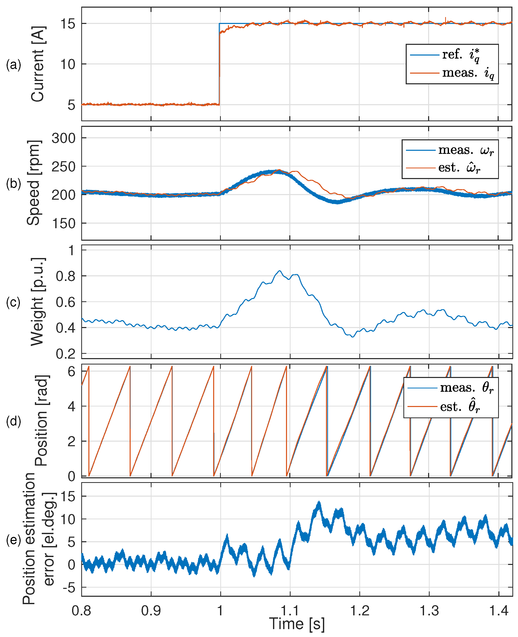
5.3.2. Dynamic Experiments of Sensorless Control Based on HFI Method

In order to evaluate the dynamic performance of the HFI-based position estimation method, a current step test and a speed acceleration test are implemented, and their experimental results are shown in Figure 14 and Figure 15, respectively.

Referring to the current step test, the tested IPMSM operates under current control, and the load motor runs under speed control. At 1.0 $\mathrm{s}$, a step current command $i_q^{*}$ from 5 $\mathrm{A}$ to 20 $\mathrm{A}$ is set to the tested IPMSM, while the rotor speed is maintained at 100 $\mathrm{srpm}$ by the load motor. From Figure 14a, the current feedback tracks the step command very well. From Figure 14d, during the dynamic process, the position estimation error is about 20 $\text{el.deg.}$ Then, with the current increased to 20 $\mathrm{A}$, the position estimation error becomes about 20 $\text{el.deg.}$

As for the speed acceleration test, the tested IPMSM operates under speed control, and the load motor works under current control. At 1.8 $\mathrm{s}$, a ramp speed command ${\omega }_r^{*}$ from 50 $\mathrm{rpm}$ to 200 $\mathrm{rpm}$ is set to the tested IPMSM, while the load motor provides a constant load torque of 0.1 $\text{N.m.}$. In Figure 15d, during the acceleration process, the position estimation error is smaller than 20 $\text{el.deg.}$

5.4. Transition between High-Speed and Low-Speed Sensorless Control

The blending algorithm of rotor position estimation between the low- and high-speed range is configured to be executed in the speed range from 160 $\mathrm{rpm}$ to 260 $\mathrm{rpm}$, which is about 10% of the rated speed. To evaluate the performance of the proposed transition algorithm, two dynamic experiments are implemented.

Firstly, a current step experiment is executed to test the dynamic performance of the transition algorithm, and the experimental results are shown in Figure 16.

Secondly, an acceleration–deceleration experiment is executed to test the performance of the transition algorithm switched between the SMO method and HFI method, and the experimental results are shown in Figure 17.

Referring to the current step test, the tested IPMSM works under current control, and the load motor runs under speed control. At 1.0 $\mathrm{s}$, a step current command $i_q^{*}$ from 5 $\mathrm{A}$ to 15 $\mathrm{A}$ is set to the tested IPMSM, while the rotor speed is maintained at 200 $\mathrm{srpm}$ by the load motor. From Figure 16a, the current feedback tracks the current step command very well. Figure 16c shows the weight coefficient used for blending the two rotor positions estimated by the SMO method and HFI method, respectively, which are proportional to the estimated rotor speed shown in Figure 16b. In Figure 16e, after the current reaches 15 $\mathrm{A}$, the error of the position estimation increases to about 7 $\text{el.deg.}$ because the blending position estimation also introduces a partial error from the HFI method, which has large position estimation error in high current load.

As for the acceleration–deceleration test, the tested IPMSM operates under speed control, and the load motor runs under current control. During 1.1 $\mathrm{s}$ to 1.4 $\mathrm{s}$, a speed command ${\omega }_r^{*}$ accelerating from 100 $\mathrm{rpm}$ to 400 $\mathrm{rpm}$ is set to the tested IPMSM, then during 3.4 $\mathrm{s}$ to 3.7 $\mathrm{s}$, the ${\omega }_r^{*}$ decelerating from 400 $\mathrm{rpm}$ to 100 $\mathrm{rpm}$ is applied to the tested IPMSM.

Due to the large inertia and friction, the actual speed lags behind the speed command, as shown in Figure 17b. However, the speed estimated by the blending algorithm tracks well with the measured speed. In Figure 17c, the weight coefficient, which is used for blending the rotor positions estimated by SMO method and HFI method, also changes promptly according to the estimated speed during the acceleration and deceleration ranges. Additionally, during the acceleration and deceleration ranges, the peaks of the position estimation error are generated as shown in Figure 17e. They are caused by the large peaks of $i_q$ in Figure 17a. However, these peaks of the position estimation error are smaller than 10 $\text{el.deg.}$, which are tolerable in sensorless control.

Summarizing from the experimental results in Figure 16 and Figure 17, it can be proven that with the proposed transition algorithm, the motor can switch smoothly between HFI-based and SMO-based position sensorless control methods.

6. Conclusions

In this paper, an SMO method for high-speed sensorless control and a rotating-voltage HFI method for low-speed sensorless control are firstly described and analyzed in detail, respectively. Then, in order to realize wide-speed-range sensorless control, a transition algorithm based on a speed-dependent weight function is designed to blend the rotor position estimated by these two methods. In this paper, plenty of experiments were implemented to test the steady-state and dynamic performance of the SMO method, HFI method, and the transition algorithm, respectively. The experimental results show that in wide-speed range the designed sensorless control strategy for an IPMSM can track the real rotor position accurately.

References

1. Xu, D.; Wang, B.; Zhang, G.; Wang, G.; Yu, Y. A review of sensorless control methods for AC motor drives. CES Trans. Electr. Mach. Syst. 2018, 2, 104–115. [Google Scholar] [CrossRef]
2. Wang, G.; Valla, M.; Solsona, J. Position Sensorless Permanent Magnet Synchronous Machine Drives—A Review. IEEE Trans. Ind. Electron. 2020, 67, 5830–5842. [Google Scholar] [CrossRef]
3. Xiao, D.; Nalakath, S.; Filho, S.R.; Fang, G.; Dong, A.; Sun, Y.; Wiseman, J.; Emadi, A. Universal Full-Speed Sensorless Control Scheme for Interior Permanent Magnet Synchronous Motors. IEEE Trans. Power Electron. 2021, 36, 4723–4737. [Google Scholar] [CrossRef]
4. Flieh, H.M.; Slininger, T.; Lorenz, R.D.; Totoki, E. Self-Sensing via Flux Injection With Rapid Servo Dynamics Including a Smooth Transition to Back-EMF Tracking Self-Sensing. IEEE Trans. Ind. Appl. 2020, 56, 2673–2684. [Google Scholar] [CrossRef]
5. Piippo, A.; Hinkkanen, M.; Luomi, J. Analysis of an Adaptive Observer for Sensorless Control of Interior Permanent Magnet Synchronous Motors. IEEE Trans. Ind. Electron. 2008, 55, 570–576. [Google Scholar] [CrossRef] [Green Version]
6. Shi, Y.; Sun, K.; Huang, L.; Li, Y. Online Identification of Permanent Magnet Flux Based on Extended Kalman Filter for IPMSM Drive With Position Sensorless Control. IEEE Trans. Ind. Electron. 2012, 59, 4169–4178. [Google Scholar] [CrossRef]
7. Chen, Z.; Tomita, M.; Doki, S.; Okuma, S. An extended electromotive force model for sensorless control of interior permanent-magnet synchronous motors. IEEE Trans. Ind. Electron. 2003, 50, 288–295. [Google Scholar] [CrossRef]
8. Boldea, I.; Paicu, M.C.; Andreescu, G.D. Active Flux Concept for Motion-Sensorless Unified AC Drives. IEEE Trans. Power Electron. 2008, 23, 2612–2618. [Google Scholar] [CrossRef]
9. Boldea, I.; Paicu, M.C.; Andreescu, G.D.; Blaabjerg, F. ‘Active Flux’ DTFC-SVM Sensorless Control of IPMSM. IEEE Trans. Energy Convers. 2009, 24, 314–322. [Google Scholar] [CrossRef]
10. Foo, G.; Sayeef, S.; Rahman, M.F. Sensorless direct torque and flux control of an IPM synchronous motor drive at low speed and standstill. In Proceedings of the 2008 Australasian Universities Power Engineering Conference, Sydney, NSW, Australia, 14–17 December 2008; pp. 1–7. [Google Scholar]
11. Zerdali, E.; Barut, M. The Comparisons of Optimized Extended Kalman Filters for Speed-Sensorless Control of Induction Motors. IEEE Trans. Ind. Electron. 2017, 64, 4340–4351. [Google Scholar] [CrossRef]
12. Yin, Z.; Gao, F.; Zhang, Y.; Du, C.; Li, G.; Sun, X. A review of nonlinear Kalman filter appling to sensorless control for AC motor drives. CES Trans. Electr. Mach. Syst. 2019, 3, 351–362. [Google Scholar] [CrossRef]
13. Chi, S.; Zhang, Z.; Xu, L. Sliding-Mode Sensorless Control of Direct-Drive PM Synchronous Motors for Washing Machine Applications. IEEE Trans. Ind. Appl. 2009, 45, 582–590. [Google Scholar] [CrossRef]
14. Wang, G.; Yang, R.; Xu, D. DSP-Based Control of Sensorless IPMSM Drives for Wide-Speed-Range Operation. IEEE Trans. Ind. Electron. 2013, 60, 720–727. [Google Scholar] [CrossRef]
15. Wang, G.; Li, Z.; Zhang, G.; Yu, Y.; Xu, D. Quadrature PLL-Based High-Order Sliding-Mode Observer for IPMSM Sensorless Control With Online MTPA Control Strategy. IEEE Trans. Energy Convers. 2013, 28, 214–224. [Google Scholar] [CrossRef]
16. Limsuwan, N.; Kato, T.; Yu, C.Y.; Tamura, J.; Reigosa, D.D.; Akatsu, K.; Lorenz, R.D. Secondary Resistive Losses With High-Frequency Injection-Based Self-Sensing in IPM Machines. IEEE Trans. Ind. Appl. 2013, 49, 1499–1507. [Google Scholar] [CrossRef]
17. Gong, L.M.; Zhu, Z.Q. A Novel Method for Compensating Inverter Nonlinearity Effects in Carrier Signal Injection-Based Sensorless Control From Positive-Sequence Carrier Current Distortion. IEEE Trans. Ind. Appl. 2011, 47, 1283–1292. [Google Scholar] [CrossRef]
18. Raca, D.; Garcia, P.; Reigosa, D.D.; Briz, F.; Lorenz, R.D. Carrier-Signal Selection for Sensorless Control of PM Synchronous Machines at Zero and Very Low Speeds. IEEE Trans. Ind. Appl. 2010, 46, 167–178. [Google Scholar] [CrossRef]
19. Bianchi, N.; Bolognani, S.; Jang, J.H.; Sul, S.K. Advantages of Inset PM Machines for Zero-Speed Sensorless Position Detection. IEEE Trans. Ind. Appl. 2008, 44, 1190–1198. [Google Scholar] [CrossRef]
20. Zhang, X.; Li, H.; Yang, S.; Ma, M. Improved Initial Rotor Position Estimation for PMSM Drives Based on HF Pulsating Voltage Signal Injection. IEEE Trans. Ind. Electron. 2018, 65, 4702–4713. [Google Scholar] [CrossRef]
21. Xu, P.L.; Zhu, Z.Q. Carrier Signal Injection-Based Sensorless Control for Permanent-Magnet Synchronous Machine Drives Considering Machine Parameter Asymmetry. IEEE Trans. Ind. Electron. 2016, 63, 2813–2824. [Google Scholar] [CrossRef]
22. Ni, R.; Xu, D.; Blaabjerg, F.; Lu, K.; Wang, G.; Zhang, G. Square-Wave Voltage Injection Algorithm for PMSM Position Sensorless Control With High Robustness to Voltage Errors. IEEE Trans. Power Electron. 2017, 32, 5425–5437. [Google Scholar] [CrossRef]
23. Kim, D.; Kwon, Y.C.; Sul, S.K.; Kim, J.H.; Yu, R.S. Suppression of Injection Voltage Disturbance for High-Frequency Square-Wave Injection Sensorless Drive With Regulation of Induced High-Frequency Current Ripple. IEEE Trans. Ind. Appl. 2016, 52, 302–312. [Google Scholar] [CrossRef]
24. Hwang, C.E.; Lee, Y.; Sul, S.K. Analysis on Position Estimation Error in Position-Sensorless Operation of IPMSM Using Pulsating Square Wave Signal Injection. IEEE Trans. Ind. Appl. 2019, 55, 458–470. [Google Scholar] [CrossRef]
25. Hua, Y.; Sumner, M.; Asher, G.; Gao, Q.; Saleh, K. Improved sensorless control of a permanent magnet machine using fundamental pulse width modulation excitation. IET Electr. Power Appl. 2011, 5, 359–370. [Google Scholar] [CrossRef] [Green Version]
26. Raute, R.; Caruana, C.; Staines, C.S.; Cilia, J.; Sumner, M.; Asher, G.M. Analysis and Compensation of Inverter Nonlinearity Effect on a Sensorless PMSM Drive at Very Low and Zero Speed Operation. IEEE Trans. Ind. Electron. 2010, 57, 4065–4074. [Google Scholar] [CrossRef]
27. Xie, G.; Lu, K.; Dwivedi, S.K.; Riber, R.J.; Wu, W. Permanent Magnet Flux Online Estimation Based on Zero-Voltage Vector Injection Method. IEEE Trans. Power Electron. 2015, 30, 6506–6509. [Google Scholar] [CrossRef]
28. Wang, G.; Kuang, J.; Zhao, N.; Zhang, G.; Xu, D. Rotor Position Estimation of PMSM in Low-Speed Region and Standstill Using Zero-Voltage Vector Injection. IEEE Trans. Power Electron. 2018, 33, 7948–7958. [Google Scholar] [CrossRef]
29. Xie, G.; Lu, K.; Dwivedi, S.K.; Rosholm, J.R.; Blaabjerg, F. Minimum-Voltage Vector Injection Method for Sensorless Control of PMSM for Low-Speed Operations. IEEE Trans. Power Electron. 2016, 31, 1785–1794. [Google Scholar] [CrossRef]
30. Zhao, C.; Tanaskovic, M.; Percacci, F.; Mariéthoz, S.; Gnos, P. Sensorless Position Estimation for Slotless Surface Mounted Permanent Magnet Synchronous Motors in Full Speed Range. IEEE Trans. Power Electron. 2019, 34, 11566–11579. [Google Scholar] [CrossRef]
31. Xie, G.; Lu, K.; Dwivedi, S.K.; Rosholm, J.R. Improved INFORM method by minimizing the inverter nonlinear voltage error effects. In Proceedings of the 2015 IEEE Workshop on Electrical Machines Design, Control and Diagnosis (WEMDCD), Turin, Italy, 26–27 March 2015; pp. 188–194. [Google Scholar]
32. Ni, R.; Lu, K.; Blaabjerg, F.; Xu, D. A comparative study on pulse sinusoidal high frequency voltage injection and INFORM methods for PMSM position sensorless control. In Proceedings of the IECON 2016—42nd Annual Conference of the IEEE Industrial Electronics Society, Florence, Italy, 23–26 October 2016; pp. 2600–2605. [Google Scholar]
33. Yang, S.C.; Hsu, Y.L. Full Speed Region Sensorless Drive of Permanent-Magnet Machine Combining Saliency-Based and Back-EMF-Based Drive. IEEE Trans. Ind. Electron. 2017, 64, 1092–1101. [Google Scholar] [CrossRef]
34. Illindala, M.; Venkataramanan, G. Frequency/Sequence Selective Filters for Power Quality Improvement in a Microgrid. IEEE Trans. Smart Grid 2012, 3, 2039–2047. [Google Scholar] [CrossRef]
35. Briz, F.; Diez, A.; Degner, M.W. Dynamic operation of carrier-signal-injection-based sensorless direct field-oriented AC drives. IEEE Trans. Ind. Appl. 2000, 36, 1360–1368. [Google Scholar] [CrossRef]
36. Secrest, C.W.; Ochs, D.S.; Gagas, B.S. Deriving State Block Diagrams That Correctly Model Hand-Code Implementation-Correcting the Enhanced Luenberger Style Motion Observer as an Example. IEEE Trans. Ind. Appl. 2020, 56, 826–836. [Google Scholar]
Figure 1. Rotor position estimation based on sliding-mode observer method.
Electronics 11 03747 g001
Figure 2. Position tracking based on phase-locked loop (PLL).
Electronics 11 03747 g002
Figure 3. High-frequency voltage injection and rotor position estimation.
Electronics 11 03747 g003
Figure 4. (a) Bandstop synchronous reference frame filter (SRFF). (b) Subtraction-based current filter to separate the fundamental and negative sequence currents from the overall measured current.
Electronics 11 03747 g004
Figure 5. Luenberger-style motion observer with heterodyning for error generation.
Electronics 11 03747 g005
Figure 6. Transition algorithm of the SMO-based position estimation and HFI-based position estimation.
Electronics 11 03747 g006
Figure 7. Test bench studied in this paper.
Electronics 11 03747 g007
Figure 8. Steady-state performance of the SMO method. (a) The operating point of ( 400 rpm , 5 A ) . (b) The operating point of ( 400 rpm , 25 A ) .
Electronics 11 03747 g008
Figure 9. Steady-state position estimation error of the SMO method at different operating points. (a) The mean value of position estimation error. (b) The peak–peak value of position estimation error.
Electronics 11 03747 g009
Figure 10. Dynamic performance of the SMO method under a step current i q * from 5 A to 15 A and constant speed 400 rpm . (a) q-axis current. (b) Rotor speed. (c) Rotor position. (d) Position estimation error.
Electronics 11 03747 g010
Figure 11. Dynamic performance of the SMO method under speed acceleration ω r * from 200 rpm to 800 rpm and constant load torque 0.1 N.m. . (a) q-axis current. (b) Rotor speed. (c) Rotor position. (d) Position estimation error.
Electronics 11 03747 g011
Figure 12. Steady-state performance of the HFI method. (a) The operating point of ( 100 rpm , 5 A ) . (b) The operating point of ( 100 rpm , 25 A ) .
Electronics 11 03747 g012
Figure 13. Steady-state position estimation error of the HFI method at different operating points. (a) The mean value of position estimation error. (b) The peak–peak value of position estimation error.
Electronics 11 03747 g013
Figure 14. Dynamic performanceof the HFI method under a step current i q * from 5 A to 20 A and constant speed 100 rpm . (a) q-axis current. (b) Rotor speed. (c) Rotor position. (d) Position estimation error.
Electronics 11 03747 g014
Figure 15. Dynamic performance of the HFI method under speed acceleration ω r * from 50 rpm to 200 rpm and constant load torque 0.1 N.m. . (a) q-axis current. (b) Rotor speed. (c) Rotor position. (d) Position estimation error.
Electronics 11 03747 g015
Figure 16. Dynamic performance of the transition algorithm under a step current i q * from 5 A to 15 A and constant speed 200 rpm . (a) q-axis current. (b) Rotor speed. (c) Weight coefficient of transition. (d) Rotor position. (e) Position estimation error.
Electronics 11 03747 g016
Figure 17. Dynamic performance of the transition algorithm under speed ω r * accelerating from 100 rpm to 400 rpm , then decelerating from 400 rpm to 100 rpm , and constant load torque 0.1 N.m. . (a) q-axis current. (b) Rotor speed. (c) Weight coefficient of transition. (d) Rotor position. (e) Position estimation error.
Electronics 11 03747 g017