Article

Food Recognition and Food Waste Estimation Using Convolutional Neural Network

by
Jelena Lubura
1,
Lato Pezo
2,*,
Mirela Alina Sandu
3,
Viktoria Voronova
4,
Francesco Donsì
5,
Jana Šic Žlabur
6,
Bojan Ribić
7,
Anamarija Peter
6,
Jona Šurić
6,
Ivan Brandić
6,
Marija Klõga
4,
Sanja Ostojić
2,
Gianpiero Pataro
5,
Ana Virsta
3,
Ana Elisabeta Oros (Daraban)
3,
Darko Micić
2,
Saša Đurović
2,8,
Giovanni De Feo
5,
Alessandra Procentese
5 and
Neven Voća
6
1
Faculty of Technology Novi Sad, University of Novi Sad, Bul. cara Lazara 1, 21000 Novi Sad, Serbia
2
Institute of General and Physical Chemistry, University of Belgrade, Studentski Trg 12-16, 11000 Beograd, Serbia
3
Faculty of Land Reclamation and Environmental Engineering, University of Agronomic Sciences and Veterinary Medicine of Bucharest, 59 Marasti Blvd, District 1, 011464 Bucharest, Romania
4
Water and Environmental Engineering Research Group, Department of Civil Engineering and Architecture, Tallinn University of Technology, Ehitajate tee 5, 19086 Tallinn, Estonia
5
Department of Industrial Engineering, University of Salerno, 84084 Fisciano, Italy
6
Faculty of Agriculture, University of Zagreb, Svetosimunska 25, 10000 Zagreb, Croatia
7
Zagreb City Holding, 10000 Zagreb, Croatia
8
Graduate School of Biotechnology and Food Industries, Peter the Great Saint-Petersburg Polytechnic University, Polytechnicheskaya street 29, 195251 Saint-Petersburg, Russia
*
Author to whom correspondence should be addressed.
Electronics 2022, 11(22), 3746; https://doi.org/10.3390/electronics11223746
Submission received: 26 October 2022 / Revised: 10 November 2022 / Accepted: 12 November 2022 / Published: 15 November 2022
(This article belongs to the Special Issue Convolutional Neural Networks and Vision Applications, Volume II)

Abstract

:
In this study, an evaluation of food waste generation was conducted, using images taken before and after the daily meals of people aged between 20 and 30 years in Serbia, for the period between 1 January and 31 April in 2022. A convolutional neural network (CNN) was employed for the tasks of recognizing food images before the meal and estimating the percentage of food waste according to the photographs taken. Keeping in mind the vast variates and types of food available, the image recognition and validation of food items present a generally very challenging task. Nevertheless, deep learning has recently been shown to be a very potent image recognition procedure, while CNN presents a state-of-the-art method of deep learning. The CNN technique was implemented to the food detection and food waste estimation tasks throughout the parameter optimization procedure. The images of the most frequently encountered food items were collected from the internet to create an image dataset, covering 157 food categories, which was used to evaluate recognition performance. Each category included between 50 and 200 images, while the total number of images in the database reached 23,552. The CNN model presented good prediction capabilities, showing an accuracy of 0.988 and a loss of 0.102, after the network training cycle. The average food waste per meal, in the frame of the analysis in Serbia, was 21.3%, according to the images collected for food waste evaluation.

1. Introduction

Food waste is currently a global problem that has come into the public and political spotlight over the past decade. Moreover, food waste is an important indicator of sustainability not only in the food production sector, but also in agriculture, as it represents the sum of resources used to produce food that is not consumed. For this reason, the disposal of food waste has negative environmental, economic and social impacts. Various studies have shown that between one third and one half of the food produced worldwide is not consumed, which has a negative impact not only on the food supply chain, but also on households [1,2,3]. It is estimated that 20% of food produced in the EU is lost or wasted [4,5]. The food industry and households in the EU alone waste around ninety million tons of food per year, or 180 kg per person, excluding losses in agriculture and fisheries [6].
According to Ref. [7], every year, 770,000 tons of food is thrown away or lost in Serbia, resulting in a profound environmental impact, but still, socio-economic awareness and the development of ecological concerns are in the initial state of development among the relevant stakeholders. Approximately 90% of the total food waste emerges in landfills, wasting precious resources, while eliminating food waste could save 580 kg CO2 eq per each ton of food waste [7]. Serbian citizens discard 350,000 tons of food every year, or 40.7 kg/capita/year, with one-third endings up in landfills, releasing large amounts of biogas instead of being used to produce energy or compost [7]. The data from this study showed that a fifth of the respondents throw leftover food directly to municipal waste containers, after which it is taken to a landfill. The second most common use of food waste is as animal feed; composting is third, while generating energy is fourth.
More than 52.9% of households discard edible parts of food less than once a week; however, 2.5% of households throw away food daily [8]. An extensive segment of society exhibits awareness and habits supporting food waste reduction, but the percentage of those individuals is still not at a satisfactory level.
The image recognition of food and food remains could present a good method to estimate food waste quantity and CO2 emissions. Still, a wide plurality of food types makes the task of optically recognizing each category of food harder, and even more so when aiming to classify a specific food item within each category [9]. Although many efforts have been made in this area, food item recognition is not yet satisfactory due to its low model accuracy (about 70%), and a wide range of the different food types available has not yet been included.
According to the literature, deep learning techniques—a collective term for algorithms which have a deep architecture for solving complex problems, such as convolutional neural networks (CNNs)—have recently been used in image recognition. CNN extracts spatial features from the image input, enabling the gathering of a number of features. Compared to CNN, using artificial neural networks (ANNs) for image recognition creates a difficulty in converting two-dimensional images into one-dimensional vectors, increasing the number of trainable parameters exponentially, which takes more storage and processing capability. The most distinctive characteristic of CNNs is their ability to automatically detect the important features of images via training, which makes the CNN a state-of-the-art technique for computer vision and image classification [10,11,12,13,14].
A food image recognition system applying the CNN model consisting of five layers has been built, and two groups of controlled trials were processed, as presented by Kagaya et al. [9]. Two datasets were used: the open dataset of 100 food class images, including about 15,000 images (UEC-FOOD100 dataset), and a fruit dataset, collected by authors, including over 40,000 images. The best accuracy achieved using the fruit dataset was 80.8%, and 60.9% was achieved using the multi-food dataset [9]. During CNN model calculation, several hyper parameters were adjusted, including the number of middle layers, the size of the convolution kernels, and the activation functions for each layer. Additionally, the optimization of these parameters, using a cuda-convnet environment, as a graphical processing unit (GPU) implementation of a CNN model was performed [10].
A smartphone application which uses a trained deep CNN model for food item recognition from a real-time image was presented in the study of Fakhrou et al. 2021 [15]. The CNN model for food recognition was trained on a customized food images dataset, with 29 varieties of food dishes and fruits [15]. The constructed model was employed in different smartphone devices for real-time prediction purposes. Devices which have an extensive hardware configuration can run the CNN model without delay and produce real-time predictions for food recognition purposes.
In this study, the recognition of food type and evaluation of the amount of food waste after the daily meals of people aged between 20 and 30 years in Serbia, for the period between 1 January and 31 April in 2022, were performed by means of convolutional neural network (CNN), with 157 different food categories. In this work, the focus was on the development of an advanced CNN for determining the probability of food category based on different images. The main idea of this study was to quantify the percentage of food waste generated as the difference between the images of plates before and after meals, with masked backgrounds, in order to increase the accuracy of and minimize background influence on the calculation.

2. Materials and Methods

2.1. Data Acquisition for Food Recognition

The images of the most common food items for the Serbian market were gathered from the internet, constituting the food item images collected (most images were downloaded from Google Images). A new image dataset was created, according to the collected images, covering 157 food categories, utilized for image recognition evaluation. Each of the food categories incorporated between 50 and 200 images, and the full set of images for image detection reached 23,552 pictures.

2.2. Food Waste Evaluation

The amount of food waste was evaluated by comparing images of the plates taken before and after the meal. The amount of food waste was expressed in percent. During this study, 1354 images were collected for food waste evaluation.

2.3. Convolutional Neural Networks

The convolutional neural network (CNN) is a class of deep learning, which is nowadays considered as one the state-of the art machine learning methods [16]. CNN represents a special kind of multi-layer perception, including many specialized hidden layers used for classification, where the neurons in the layers are self-optimized by learning. CNN is mainly used for clustering the images by their similarity and classifying images; compared to other image classification algorithms, CNN uses minor pre-processing. Three layers form the architecture of CNN, and these are the convolutional layer, pooling layer and fully connected layer [17,18,19,20,21,22,23,24], presented in Figure 1.
The CNN has two crucial processes that make its convolutional neural networks different from other neural networks: convolution and sampling. In the CNN’s convolutional layers, units are structured into feature maps and connected via a filter to local patches in the previous layer feature map, where the visual features from the input image are extracted by locally trained filters. Feature maps are reduced by the pooling operation, becoming the input images for the next convolution. The process continues until deep features are extracted and, after these steps, a decision is typically made by a classifier of these features. The fully connected layer frequently ends with a non-linear function, usually a Softmax output layer for classification purposes, creating the class scores from the activations that are used for the classification [25].

2.3.1. Convolution

The convolution operation is responsible for detecting the edges and features of the images. The convolution layer is a structure consisting of a great number of fixed-size filters and allowing complex functions to be applied to the input image. The locally trained filters slide over the image and carry out the convolutional process, where every filter has the same bias and weight values; this is called the weight sharing mechanism, which provides the ability to represent the same feature across the whole image. The weight sharing ability of the convolutional operation enables the extraction of different sets of features within an image, using a sliding kernel with the same set of weights on an image, and by making the CNN as efficient as a fully connected network [26]. Every neuron is connected with the previous layer through the area of the neuron local receptive field, the size of which is determined by the size of the filters [27]. If m × n and c × c are the size of the input image and kernel, respectively; i is the image; and b and w are the filter bias and weight, respectively, then the output can be calculated as in Equation (1) [28].
O 0 , 0 = f b + k = 0 c j = 0 c w k , j i 0 + k , 0 + j
where f is the activation function; the frequently used function is the rectified linear unit (ReLU) function, which behaves linearly for positive inputs and returns zero values for both negative and zero inputs, as in Equation (2) [29].
f ( x ) = 0 ; f o r   x < 0 ; f ( x ) = x ; f o r   x 0
The output of the convolutional layer is passed through the ReLU function, which performs an elementwise activation to the output that is produced by the preceding layer [30].

2.3.2. Pooling

The pooling operation is an important concept in convolutional neural networks which performs non-linear downsampling, and it is applied to feature maps that have passed through the convolution and activation function, enabling smaller feature maps to be generated which represent summaries of the input feature maps [31]. Mostly, the convolutional layer is followed by a pooling layer, which is performed by sliding a window on the image in order to apply the selected operation. In the pooling layer, the input feature map is summarized by pooling operators such as stochastic, max and mean pooling. Stochastic pooling means that the activation function within the active pooling region is randomly selected. The max pooling represents the choosing of the maximum number of feature map nodes within the kernel [32], while the mean pooling takes the mean of the input values [33]. Max pooling provides benefits in eliminating minimum values which the reduce computations for upper layers, providing robustness while reducing the dimensions of the intermediate feature maps. The major advantages of the pooling process are image size reduction and independent visual features extraction [34,35].

2.3.3. Fully Connected Layer

After the completion of the convolution and pooling operations, the output data are transformed into a one-dimensional vector representing the input of the fully connected layer, which can contain one or more hidden layers. In these layers, neurons multiply the sum of the weighted inputs and biases, where the calculated value passes through the activation function.

2.3.4. Output Layer

In the output layer, the Softmax function provides class labels probability, where the idea of logistic regression for multiclass problems is generalized [36]. The class labels probability is calculated using the Softmax function, as in Equation (3) [37,38,39].
o ( j ) = e f k j = 1 N f k 1 ( j )
where the o(j) is the jth output of the Softmax function, fk represents the last layer, N is the number of classes, and j is the jth neuron at fk.

2.3.5. Proposed CNN Model

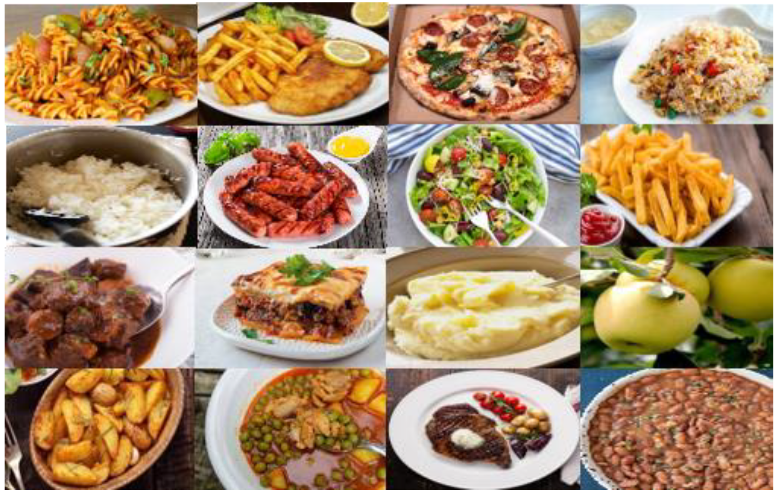
The proposed model was built using Keras, an API for deep learning methods which uses the Python programming language. Keras runs on the backend platform, Tensorflow. The images for training the CNN model were sorted into 157 different food categories, where each category contained 50 to 200 images, and the total number of images was 23,552. The food categories were selected based on Serbian students’ eating habits, and examples of the food images used to train the model are presented in Figure 2.
As CNN needs only minor pre-processing, the imported data were previously sorted into food categories and each image size was reduced in size (100 pixels) in order to achieve faster calculation, with the caution that it can cause less accurate prediction. In addition, each image was assigned with an index regarding the category to which it belongs. Images were randomly divided for training and testing the model. In the proposed method, the sequential model was used and the model was built as in Figure 1. In order to extract the deep features, the proposed CNN model contains two convolutional layers. In the first convolution layer, 32 filters were used with a size of 3 × 3 and the ReLU activation function, while in the second convolution, 64 filters were used with the same size, and the activation function as in the first layer. The filter in both pooling operations had the size of 2 × 2. The fully connected layer consisted of 64 neurons, activated with the ReLU activation function, while the second fully connected layer, i.e., the output layer with 157 neurons, with the Softmax activation function was used to sort the images into categories and, as a result, provide the probability for each category. Softmax is a continuously differentiable function (Equation (4)), which allows the calculation of the loss function derivative with respect to every weight in the neural network and the adjustment of the weights accordingly in order to minimize the loss function [40].
f ( x ) = ln 1 + e x
The model was compiled using an adaptive moment estimation (Adam) optimizer and loss function sparse categorical cross-entropy. The model was fitted in 20 epochs in order to avoid overfitting, where, for fitting, it used the data to train the model.
The Adam optimizer is commonly used due to its high calculation efficiency and low calculation memory requirements, and it is well suited for the problems of non-stationary global optimization with strong noise, sparse gradient and large-scale hyper-parameters. Furthermore, the learning rates of different hyperparameters can be adaptively tuned by imposing dynamic constrains, where each hyperparameter has its own learning rate, enabling accelerated convergence and improving the training effect. The Adam optimizer was used for CNN loss function minimization and for searching the global optimal solution, in order to obtain optimized network hyperparameters, including the convolution kernel and bias [41,42,43].
Since image prediction is a common classification problem, sparse categorical cross-entropy was adopted as the loss function (Equation (5)) [40].
Sparse   categorical   cross   entropy = i = 1 N j = 1 M p j i log e g e q j i
where p j i represents the class true probability distribution for the training sample i, q j i denotes the class predicted probability distribution for the training sample i, N is the number of training samples and M is the number of classes.

2.4. Food Waste Calculation

The main focus of this research was to quantify the food waste from plate images before and after the meal, while the background can vary in the images, because, frequently, things on the table can be changed in position, resulting in the necessity for background removal.
Background removal needs to be considered in order to segment objects from an image, which can be done manually or semi-manually, while the automatic background removal is a challenging task. The most popular background removal techniques are foreground detection, the machine learning-based approach and edge-based background removal. The foreground detection technique detects changes in the image sequence and uses background subtraction to separate the foreground from an image. The machine learning-based approach uses various machine learning algorithms to separate the foreground from the background. The edge-based background removal technique detects edges in the image and, based on these, finds a continuous edge path, while all the elements outside the path are considered as the background [44,45,46]. In this work, background removal was performed using the edge-based background removal technique, which attempts to find the contrast lines or edges in an image, which is the first step in pre-processing the image in order to differentiate objects. When the edges are detected, defining contours becomes accurate, and in the computer vision, contours represent the continuous boundary lines between areas of color contrasting or intensity. Contrary to edge detection, finding contours enables shapes to be found within the image.
During the image pre-processing, the important step is to convert the image into grayscale and use the converted image for the edge detection and finding the contours, where contours that are too big or small to be the foreground are removed and the remaining contours are considered the foreground. Small details in the background can generate very small contours, while on the contrary, very large contours are expected to be seen as a visual artefact of the background. A final background is generated from the remaining contours and blended into the original image.
The main influence on the background removal is the set of assigned variables, in which each variable has a unique effect, as explained in Table 1.
The minimum intensity value (low canny variable) dictates how sensitive contrast must be in order to be detected; if it is adjusted to be too low, it may result in more edges than necessary. The maximum intensity value (high canny) classifies every contrast above its value to be an edge; if it is adjusted to be very high, it can affect performance, while on the other hand, a low value can mean the significant edges are missed. The step of dilating and eroding the edges is optional, but this can pronounce the edges more and create a finer background contour. Lastly, the mask and the frame are blended together with a black background [47].
The same procedure was performed for both plate images before and after the meal, in order to compare their absolute differences and determine the food waste. The food waste was calculated using the simple “absdiff” function [48].

3. Results and Discussion

3.1. CNN Model Results

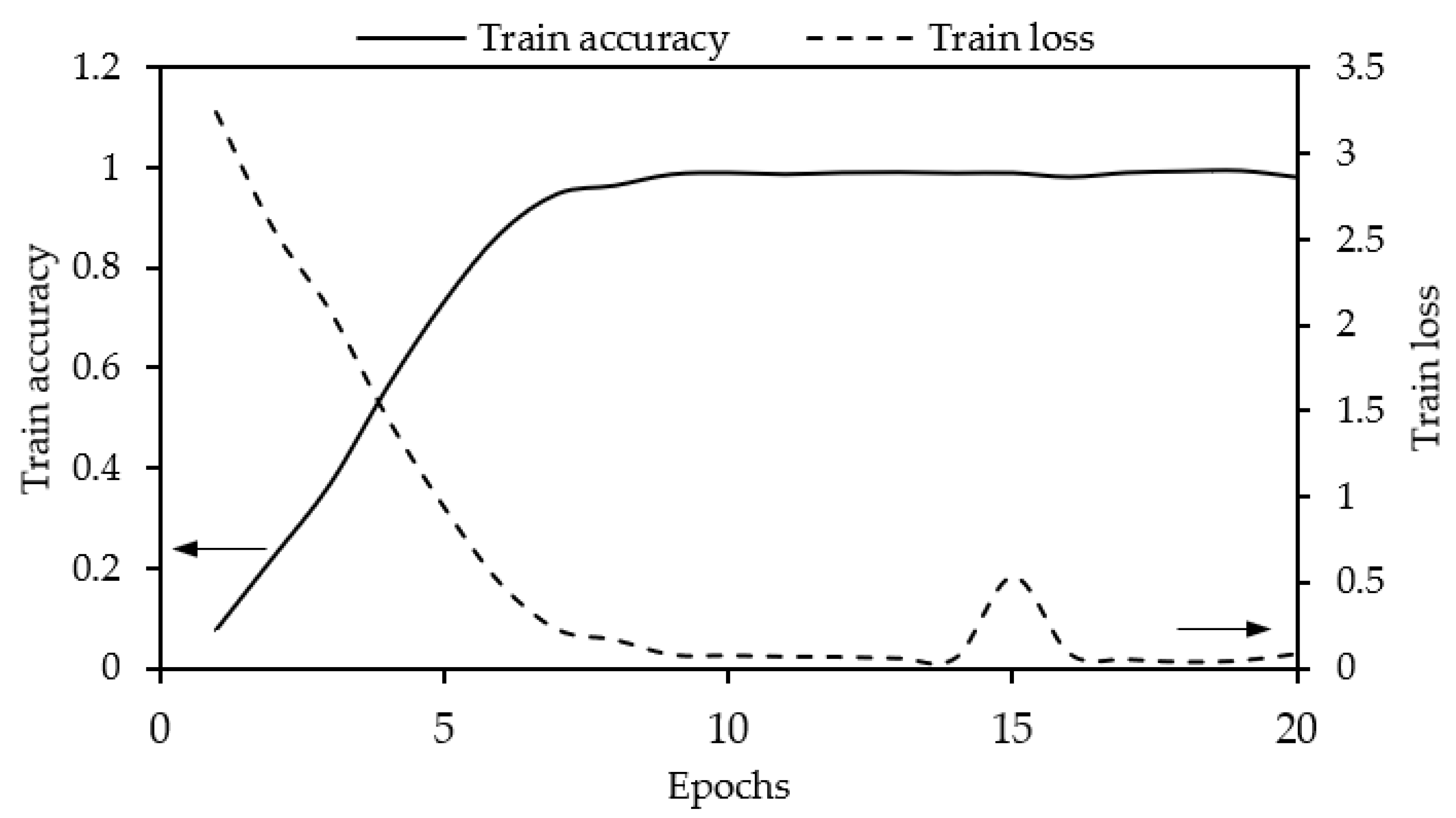
The model was trained for 20 epochs, and the training results, i.e., train accuracy and loss, are presented in Figure 3.
The training accuracy increased with the epoch’s number increment until the 10th epoch, when it was almost constant. The highest train accuracy and lowest train loss were detected for the 19th epoch, after which a slight train accuracy increase and train loss decrease were observed due to overfitting. More than 20 epochs for training would cause high overfitting, and 10 epochs would be enough to achieve high model accuracy without any risk of overfitting. The test accuracy and loss after the training were 0.988 and 0.102, respectively.
The predicted food category is accurate, showing a not-dominant probability for other categories. In order to better explain the results of the recognition of different foods, 157 categories of food were regrouped into 12 composite food categories, which could be presented within a single table. The proposed composite food categories were fruit, vegetable, processed fruits and vegetables, potatoes, pasta, rice and cereal, meat and meat products, fish, milk and dairy products, bread, cookies, prepared meals and other. Each of the 12 composite food categories consisted of several food categories presented in the database of 157 food categories. For instance, the composite food category named “Fruit” consisted of food categories such as “apple”, “pear”, “strawberry”, “banana” and “peach”.
The proposed CNN model calculates the probability of each food item grouped in one of the twelve composite food categories to be correctly recognized; see Table 2. The results shown in Table 2 contain the average of the probabilities that the picture of each food item is correctly recognized, within a composite category. For example, the probability of the correct recognition of the “Fruit” category is the average of the probabilities that the pictures of apples, pears, strawberries, bananas, peaches, etc., were correctly recognized.
It can be observed that the predicted composite food categories were accurate, showing a not-dominant probability for the other composite categories.
The proposed CNN model can be improved by increasing the data for training the model, the image size, the number of deep layers and the number of epochs. However, increasing the image size and number of layers can be time-consuming, and in addition, increasing the number of layers and epochs can cause overfitting.

3.2. Food Waste Evaluation Results

The surface around the largest shape of the plate’s images before and after the meal was masked, and the food waste was calculated as the difference between the masked images. Figure 4a,b show the plate images originally taken before and after meal, respectively. Figure 4c,d show the images before and after the meal with a masked background, respectively, where the black color represents the mask. Additionally, Figure 4e shows the area of two images, which was taken into consideration while calculating the image differences. As can be seen in Figure 4, the result of the model is that 95.5% of food was eaten, while 4.5% of food was considered as waste, which seems to be in accordance with the presented images.
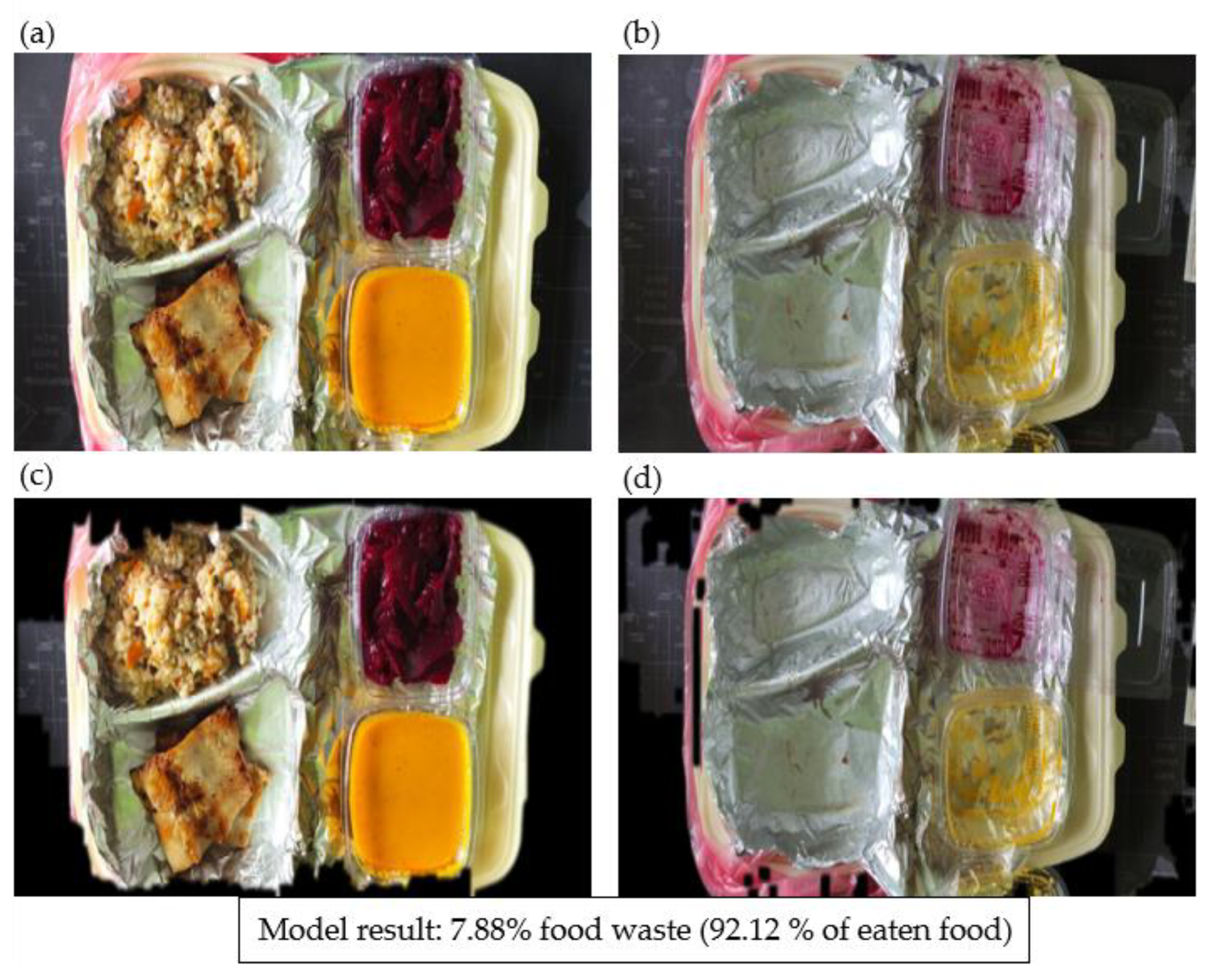
The food not placed on the plates represents a challenging test of model accuracy. As can be seen in Figure 5, the food is located in plastic boxes, and altogether in a bigger box. As the model masked the biggest shape, in this example, the big box was masked. This problem occurs in the difference between the images before and after the meal, due to the position of the small plastic boxes. Before the meal (Figure 5a), the plastic boxes were closed and the background was masked, while after the meal, they were opened and masking was conducted around them, causing a difference not related to the food waste. The model gave the result that 7.88% of food is waste, although it needs to be taken into the consideration that this percentage might not be completely accurate due to the above explained problem with the open plastic box.
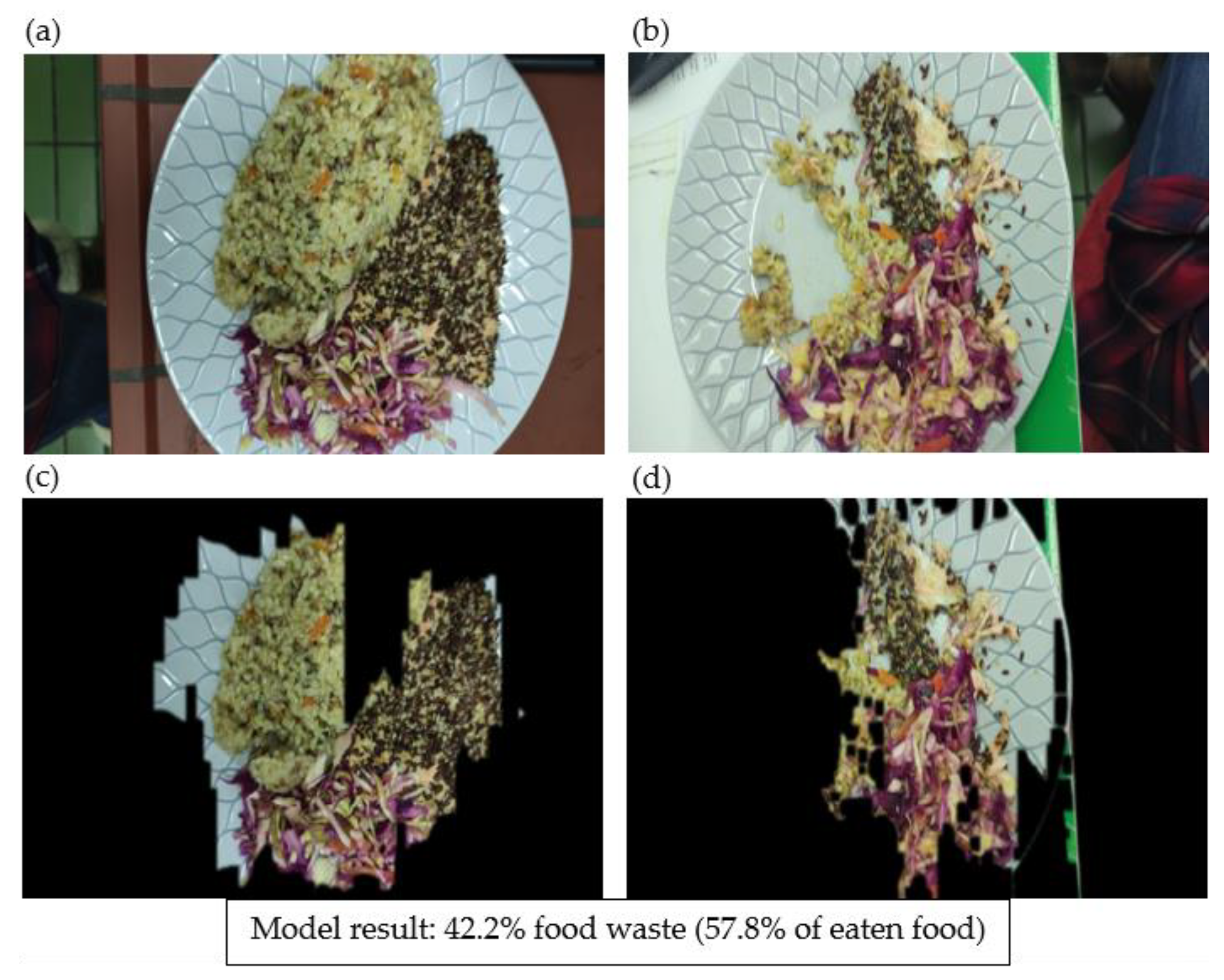
Since the model finds the biggest contour on the image and masks everything outside the contour found, and this is considered the background, a problem occurs with plates with shapes. Figure 6 presents one deficiency of the model for food waste calculation, where one part of the plate is recognized as background and the other part as a food. The model is unable to distinguish the contour of the plate and the food, leading to inaccurate food waste calculation; in this case, food waste was detected to be 57.8%. The problem of plates with shapes can be solved if the whole plate is shown in the image; then, the model would find the plate to be the biggest contour, and not the part of the food.
Another deficiency of the model is presented in Figure 7, where the plate has an irregular shape, leading to difficulties in finding the biggest contour and masking the background. The irregular plates caused inadequate food waste detection results, in this case producing the figure of 37.4%.
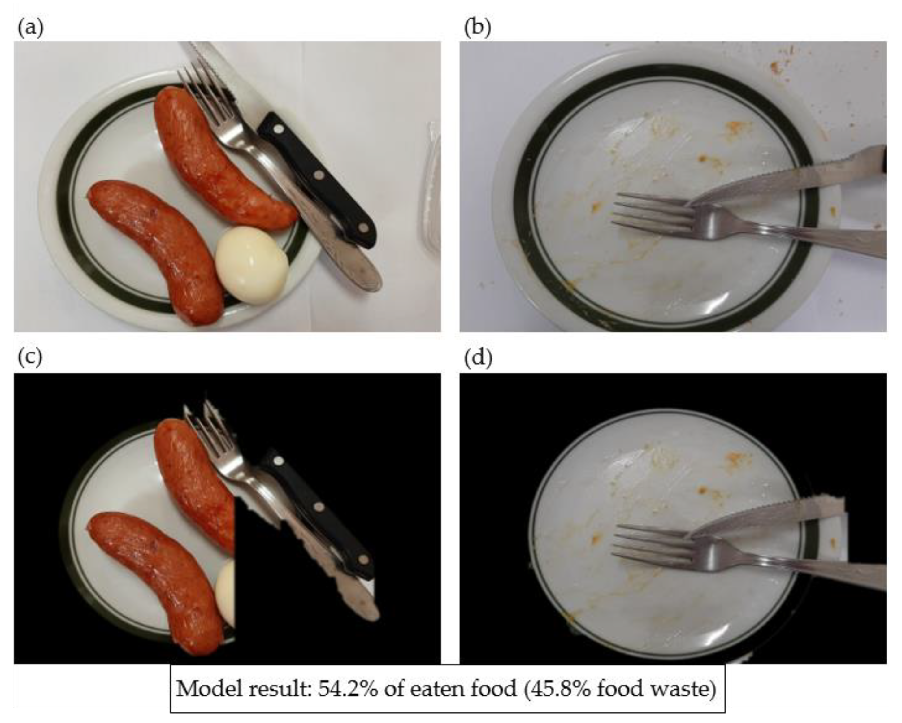
The last deficiency of the proposed model is detected when the cutlery is part of the plate in the image before the meal, and when, after the meal, the cutlery is positioned in the middle of the plate. In this case, the cutlery is detected as part of the food before meal and the food waste in the images after the meal. Observing Figure 8a,b, with common sense, it can be concluded that there is 0% food waste; however, the model recognized the cutlery as food, and the model produced false result of 45.8% of food waste.
The food waste calculations were performed based on students’ plate images from the Republic of Serbia, and the results are presented in Table 3, where the average food waste is presented. Considering the previously explained model issues, it can be assumed that the food waste results presented in Table 3 are less accurate than those calculated using the model, as all the previously explained irregularities were also included in the students’ images.
The variety of food waste percentage from different students might be due to the previously explained model deficiencies or inaccurate images.
The average food waste among the students was calculated and the results showed that 21.3% of food was wasted, which can be considered as quite a high number. On the other hand, the authors believe that a more thorough examination could be performed to examine whether the images contained edible or non-edible parts of food.
The proposed model for calculating food waste is recommended for usage with plain plates, without colors and asymmetrical shapes, where adequate plate visibility is enabled. The proposed model for determining probability and calculating the food waste based on images is novel and should improve self-consciousness among students about the generation of food waste.

4. Conclusions

A CNN model for determining the probability of different food categories based on images was developed with high accuracy (more than 98%). Moreover, students’ images of plates before and after their meals were analyzed by masking the background, in order to calculate the differences between the two images without any background, which is considered eaten food, and the food waste was calculated as the rest, up to 100%. The calculation efficiency is dependent on the accuracy of the proposed model. The model showed accurate results when the whole plate is seen in the image, and also when the plate is simple, without irregular colors or shapes. Additionally, any non-food objects (e.g., cutlery) should be excluded from the images. It was calculated that the food waste of Serbian students amounted to 21.3%. Although the model has its deficiencies, when using the model properly, the food waste is calculated using a fast and accurate novel approach.

Author Contributions

Conceptualization, J.L., L.P., B.R., J.Š.Ž. and N.V.; methodology, J.L. and N.V.; software, J.L. and L.P.; validation, N.V.; formal analysis, J.L.; investigation, J.L., A.P. (Anamarija Peter), J.Š., I.B., M.A.S., A.V., A.E.O., S.O., D.M., S.Đ., F.D., G.D.F., G.P. and A.P. (Alessandra Procentese); resources, J.L., L.P., A.P. (Anamarija Peter), J.Š., I.B. and N.V.; data curation, J.L. and L.P.; writing—original draft preparation, J.L., L.P., V.V., M.K., M.A.S., F.D. and N.V.; writing—review and editing J.L., L.P., V.V., M.K., M.A.S., F.D. and N.V.; visualization, J.L. and L.P.; supervision, V.V., M.K., M.A.S., F.D. and N.V.; project administration, J.Š.Ž., V.V., M.K., M.A.S., F.D. and N.V.; funding acquisition, L.P., V.V., M.K., M.A.S., F.D. and N.V. All authors have read and agreed to the published version of the manuscript.

Funding

This research was funded by project “Zero food waste education of “Z” generation of European citizens (ZeeWaste4EU)”, Grant Agreement Number: 2021-1-HR01-KA220-HED-000023012, Erasmus+ programme, Action Type KA220-HED—Cooperation partnerships in higher education.

Conflicts of Interest

The authors declare no conflict of interest.

References

  1. Bio Intelligence Service. Preparatory Study on Food Waste across EU 27: Final Report. Publications Office. 2011. Available online: https://data.europa.eu/doi/10.2779/85947 (accessed on 2 October 2021).
  2. Food and Agriculture Organization of the United Nations. Global Initiative on Food Loss and Waste. 2017. Available online: http://www.fao.org/3/i7657e/i7657e.pdf (accessed on 2 October 2021).
  3. Gustavsson, J.; Cederberg, C.; Sonesson, U. Global Food Losses and Food Waste: Extent, Causes and Prevention. In Study Conducted for the International Congress Save Food! at Interpack, 16–17 May 2011; Food and Agriculture Organization of the United Nations: Düsseldorf, Germany, 2011; Available online: http://www.fao.org/3/mb060e/mb060e.pdf (accessed on 2 October 2021).
  4. European Commission. Communication Closing the loop—An EU Action Plan for the Circular Economy. 2015. Available online: https://eurlex.europa.eu/legal-content/EN/TXT/HTML/?uri=CELEX:52015DC0614&from=LT (accessed on 2 October 2021).
  5. Stenmarck, Å.; Jensen, C.; Quested, T.; Moates, G.; Buksti, M.; Cseh, B.; Juul, S.; Parry, A.; Politano, A.; Redlingshofer, B.; et al. Estimates of European Food Waste Levels, Reducing food waste through social innovation, Fusions EU project, European Commission (FP7), Coordination and Support Action –CSA, Grant Agreement no. 311972. 2016. [CrossRef]
  6. Zębek, E.; Žilinskienė, L. The legal regulation of food waste in Poland and Lithuania in compliance with EU directive 2018/851. Entrep. Sustain. Issues 2021, 9, 221–238. [Google Scholar] [CrossRef]
  7. Ministerie van Landbouw, Natuur en Voedselkwaliteit. Available online: https://www.agroberichtenbuitenland.nl/actueel/nieuws/2021/09/24/serbia-food-waste (accessed on 15 September 2022).
  8. United Nations Serbia. Available online: https://serbia.un.org/en/158555-how-why-and-how-much-do-we-throw-food-away (accessed on 15 September 2022).
  9. Kagaya, H.; Aizawa, K.; Ogawa, M. Food detection and recognition using convolutional neural network. In Proceedings of the 22nd ACM international conference on Multimedia, Orlando, FL, USA, 3 November 2014. [Google Scholar]
  10. Zhang, W.; Zhao, D.; Gong, W.; Li, Z.; Lu, Q.; Yang, S. Food image recognition with convolutional neural networks. In Proceedings of the 2015 IEEE 12th International Conference on Ubiquitous Intelligence and Computing and 2015 IEEE 12th International Conference on Autonomic and Trusted Computing and 2015 IEEE 15th International Conference on Scalable Computing and Communications and Its Associated Workshops (UIC-ATC-ScalCom), Beijing, China, 15 August 2015. [Google Scholar]
  11. Chauhan, R.; Ghanshala, K.K.; Joshi, R.C. Convolutional neural network (CNN) for image detection and recognition. In Proceedings of the 2018 First International Conference on Secure Cyber Computing and Communication (ICSCCC), Jalandhar, India, 15th December 2018. [Google Scholar]
  12. Wu, M.; Chen, L. Image recognition based on deep learning. In Proceedings of the 2015 Chinese Automation Congress (CAC), Wuhan, China, 27 November 2015. [Google Scholar]
  13. Cheng, F.; Zhang, H.; Fan, W.; Harris, B. Image Recognition Technology Based on Deep Learning. Wirel. Pers. Commun. 2018, 102, 1917–1933. [Google Scholar] [CrossRef]
  14. Traore, B.B.; Kamsu-Foguem, B.; Tangara, F. Deep convolution neural network for image recognition. Ecol. Inform. 2018, 48, 257–268. [Google Scholar] [CrossRef] [Green Version]
  15. Fakhrou, A.; Kunhoth, J.; Al Maadeed, S. Smartphone-based food recognition system using multiple deep CNN models. Multimedia Tools Appl. 2021, 80, 33011–33032. [Google Scholar] [CrossRef]
  16. Nath, S.; Naskar, R. Automated image splicing detection using deep CNN-learned features and ANN-based classifier. Signal, Image Video Proc. 2021, 15, 1601–1608. [Google Scholar] [CrossRef]
  17. Agha, R.A.A.R.; Sefer, M.N.; Fattah, P. A comprehensive study on sign languages recognition systems using (SVM, KNN, CNN and ANN). In Proceedings of the First International Conference on Data Science, E-learning and Information Systems, Madrid, Spain, 1 October 2018. [Google Scholar] [CrossRef]
  18. Kareem, S.; Hamad, Z.J.; Askar, S. An evaluation of CNN and ANN in prediction weather forecasting: A review. Sustain. Eng. Innov. 2021, 3, 148–159. [Google Scholar] [CrossRef]
  19. Anwar, S.M.; Majid, M.; Qayyum, A.; Awais, M.; Alnowami, M.; Khan, M.K. Medical Image Analysis using Convolutional Neural Networks: A Review. J. Med. Syst. 2018, 42, 226. [Google Scholar] [CrossRef] [Green Version]
  20. Brodrick, P.G.; Davies, A.B.; Asner, G.P. Uncovering Ecological Patterns with Convolutional Neural Networks. Trends Ecol. Evol. 2019, 34, 734–745. [Google Scholar] [CrossRef]
  21. Sameen, M.I.; Pradhan, B.; Lee, S. Application of convolutional neural networks featuring Bayesian optimization for landslide susceptibility assessment. CATENA 2019, 186, 104249. [Google Scholar] [CrossRef]
  22. Hasan, M.; Ullah, S.; Khan, M.J.; Khurshid, K. Comparative Analysis of SVM, Ann and Cnn for Classifying Vegetation Species Using Hyperspectral Thermal Infrared Data. Int. Arch. Photogramm. Remote Sens. Spatial Inf. Sci. 2019, XLII-2/W13, 1861–1868. [Google Scholar] [CrossRef] [Green Version]
  23. Ravi, D.; Wong, C.; Deligianni, F.; Berthelot, M.; Andreu-Perez, J.; Lo, B.; Yang, G.-Z. Deep Learning for Health Informatics. IEEE J. Biomed. Health Inform. 2016, 21, 4–21. [Google Scholar] [CrossRef] [PubMed] [Green Version]
  24. Kamilaris, A.; Prenafeta-Boldú, F.X. A review of the use of convolutional neural networks in agriculture. J. Agric. Sci. 2018, 156, 312–322. [Google Scholar] [CrossRef] [Green Version]
  25. Gu, J.; Wang, Z.; Kuen, J.; Ma, L.; Shahroudy, A.; Shuai, B.; Liu, T.; Wang, X.; Wang, G.; Cai, J.; et al. Recent advances in convolutional neural networks. Pattern Recognit. 2018, 77, 354–377. [Google Scholar] [CrossRef] [Green Version]
  26. Khan, A.; Sohail, A.; Zahoora, U.; Qureshi, A.S. A survey of the recent architectures of deep convolutional neural networks. Artif. Intell. Rev. 2020, 53, 5455–5516. [Google Scholar] [CrossRef] [Green Version]
  27. Zhou, D.-X. Theory of deep convolutional neural networks: Downsampling. Neural Netw. 2020, 124, 319–327. [Google Scholar] [CrossRef] [PubMed]
  28. Sarıgül, M.; Ozyildirim, B.; Avci, M. Differential convolutional neural network. Neural Netw. 2019, 116, 279–287. [Google Scholar] [CrossRef]
  29. Aghdam, H.H.; Jahani Heravi, E. Guide to Convolutional Neural Networks; Springer International Publishing: New York, NY, USA, 2017; pp. 973–978. [Google Scholar]
  30. Sarigul, M.; Ozyildirim, B.M.; Avci, M. Deep Convolutional Generalized Classifier Neural Network. Neural Proc. Lett. 2020, 51, 2839–2854. [Google Scholar] [CrossRef]
  31. Kiranyaz, S.; Avci, O.; Abdeljaber, O.; Ince, T.; Gabbouj, M.; Inman, D.J. 1D convolutional neural networks and applications: A survey. Mech. Syst. Signal Proc. 2020, 151, 107398. [Google Scholar] [CrossRef]
  32. Lee, H.; Kwon, H. Going Deeper with Contextual CNN for Hyperspectral Image Classification. IEEE Trans. Image Proc. 2017, 26, 4843–4855. [Google Scholar] [CrossRef] [Green Version]
  33. Sun, Y.; Xue, B.; Zhang, M.; Yen, G.G.; Lv, J. Automatically Designing CNN Architectures Using the Genetic Algorithm for Image Classification. IEEE Trans. Cybern. 2020, 50, 3840–3854. [Google Scholar] [CrossRef] [Green Version]
  34. Hussain, M.; Bird, J.J.; Faria, D.R. A Study on CNN Transfer Learning for Image Classification. In UK Workshop on Computational Intelligence; Springer: Cham, Switzerland, 2018; pp. 191–202. [Google Scholar]
  35. Li, Z.; Liu, F.; Yang, W.; Peng, S.; Zhou, J. A Survey of Convolutional Neural Networks: Analysis, Applications, and Prospects. IEEE Trans. Neural Networks Learn. Syst. 2021, 1, 1–21. [Google Scholar] [CrossRef] [PubMed]
  36. Kakarla, J.; Isunuri, B.V.; Doppalapudi, K.S.; Bylapudi, K.S.R. Three—Class classification of brain magnetic resonance images using average—Pooling convolutional neural network. Int. J. Imaging Syst. Technol. 2021, 31, 1731–1740. [Google Scholar] [CrossRef]
  37. Kuo, C.-C.J. Understanding convolutional neural networks with a mathematical model. J. Vis. Commun. Image Represent. 2016, 41, 406–413. [Google Scholar] [CrossRef] [Green Version]
  38. Yiğit, G.; Ozyildirim, B.M. Comparison of convolutional neural network models for food image classification. J. Inf. Telecommun. 2017, 2, 347–357. [Google Scholar] [CrossRef]
  39. Zhang, Q.; Zhang, M.; Chen, T.; Sun, Z.; Ma, Y.; Yu, B. Recent advances in convolutional neural network acceleration. Neurocomputing 2018, 323, 37–51. [Google Scholar] [CrossRef] [Green Version]
  40. Yin, X.; Liu, Q.; Huang, X.; Pan, Y. Real-time prediction of rockburst intensity using an integrated CNN-Adam-BO algorithm based on microseismic data and its engineering application. Tunn. Undergr. Space Technol. 2021, 117, 104133. [Google Scholar] [CrossRef]
  41. Guzmán-Torres, J.A.; Domínguez-Mota, F.J.; Alonso-Guzmán, E.M. A multi-layer approach to classify the risk of corrosion in concrete specimens that contain different additives. Case Stud. Constr. Mater. 2021, 15, e00719. [Google Scholar] [CrossRef]
  42. Taqi, A.M.; Awad, A.; Al-Azzo, F.; Milanova, M. The Impact of Multi-Optimizers and Data Augmentation on TensorFlow Convolutional Neural Network Performance. In Proceedings of the IEEE 1st Conference on Multimedia Information Processing and Retrieval, Miami, FL, USA, 18 April 2018; pp. 140–145. [Google Scholar]
  43. Menaka, D.; Vaidyanathan, S.G. Chromenet: A CNN architecture with comparison of optimizers for classification of human chromosome images. Multidimens. Syst. Signal Process. 2022, 33, 747–768. [Google Scholar] [CrossRef]
  44. Fang, W.; Ding, Y.; Zhang, F.; Sheng, V.S. DOG: A new background removal for object recognition from images. Neurocomputing 2019, 361, 85–91. [Google Scholar] [CrossRef]
  45. Feng, X.; Pei, W.; Jia, Z.; Chen, F.; Zhang, D.; Lu, G. Deep-Masking Generative Network: A Unified Framework for Background Restoration from Superimposed Images. IEEE Trans. Image Proc. 2021, 30, 4867–4882. [Google Scholar] [CrossRef]
  46. Wang, X.; Tang, J.; Whitty, M. Side-view apple flower mapping using edge-based fully convolutional networks for variable rate chemical thinning. Comput. Electron. Agric. 2020, 178, 105673. [Google Scholar] [CrossRef]
  47. Wu, J.; Yin, J.; Zhang, Q. Institute of Electrical and Electronics Engineers. In Proceedings of the IEEE 13th International Conference on Electronic Measurement & Instruments, Yangzhou, China, 20–22 October 2017. [Google Scholar]
  48. Parveen, S.; Shah, J. A Motion Detection System in Python and Opencv. In Proceedings of the 3rd International Conference on Intelligent Communication Technologies and Virtual Mobile Networks, ICICV 2021, Tirunelveli, India, 4–6 February 2021; pp. 1378–1382. [Google Scholar]
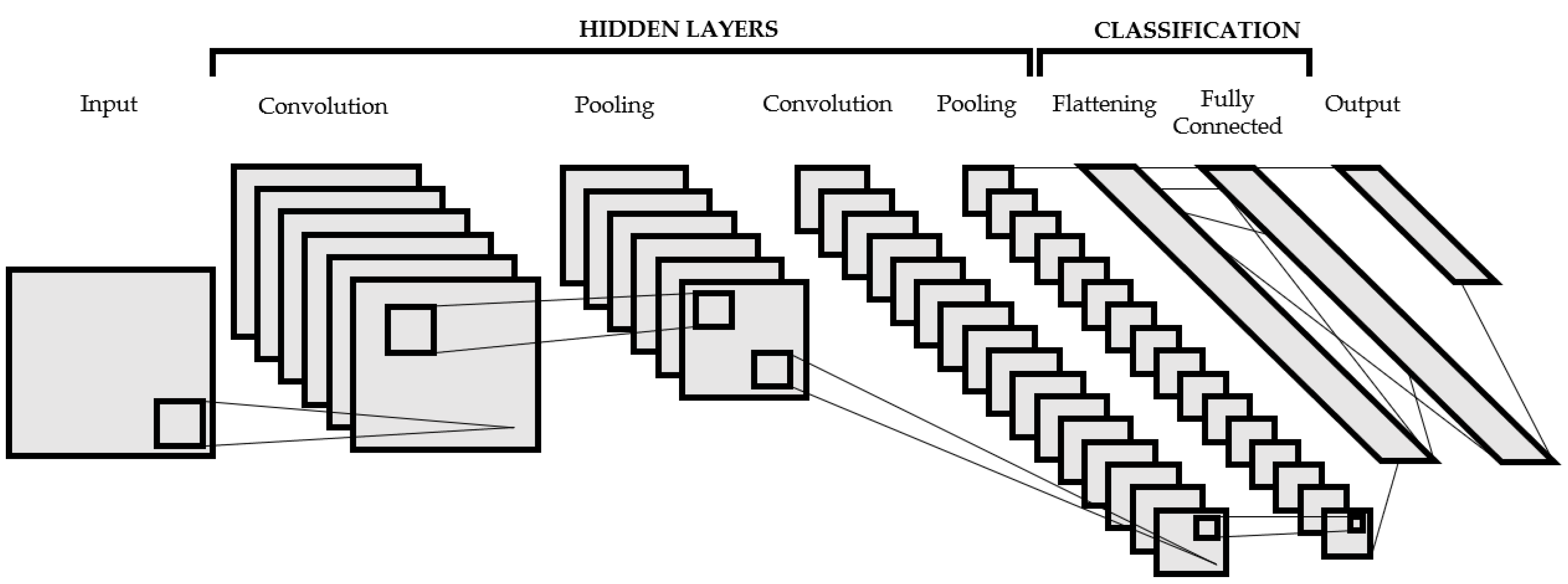
Figure 1. CNN architecture.
Electronics 11 03746 g001
Figure 2. Examples of images used for training the CNN model.
Electronics 11 03746 g002
Figure 3. Training results per epoch.
Electronics 11 03746 g003
Figure 4. The example of images (a) before the meal, (b) after the meal, (c) before the meal and masked and (d) after the meal and masked.
Electronics 11 03746 g004
Figure 5. The example of images in plastic boxes (a) before the meal, (b) after the meal, (c) before the meal and masked and (d) after the meal and masked.
Electronics 11 03746 g005
Figure 6. The model deficiency caused by the shape of the plate; (a) before the meal, (b) after the meal, (c) before the meal and masked and (d) after the meal and masked.
Electronics 11 03746 g006
Figure 7. The model deficiency due to the color and shape of the plate; (a) before the meal, (b) after the meal, (c) before the meal and masked and (d) after the meal and masked.
Electronics 11 03746 g007
Figure 8. The model deficiency caused by cutlery after the meal; (a) before the meal, (b) after the meal, (c) before the meal and masked and (d) after the meal and masked.
Electronics 11 03746 g008
Table 1. The background removal’s set of variables and their descriptions and assigned values.
VariableDescriptionAssigned Value
BlurAffects the smoothness of the dividing line between the background and foreground21
Low cannyThe minimum intensity for drawing the edges10
High canny The maximum intensity for drawing the edges200
Dilation iterationThe dilation’s number of iteration for masking10
Erode iterationThe erosion’s number of iteration for masking10
Mask colorThe masked background color(0, 0, 0)
Table 2. Confusion matrices for proposed CNN model with average composite food category percentage probability.
FruitVegetableProcessed Fruits and VegetablesPotatoesPasta, Rice, CerealMeat and Meat ProductsFishMilk and Dairy ProductsBreadCookiesPrepared MealsOther
Fruit99.92.8 × 10−142.2 × 10−171.2 × 10−206.1 × 10−91.0 × 10−121.4 × 10−61.4 × 10−53.5 × 10−221.2 × 10−32.9 × 10−159.8 × 10⁻²
Vegetable1.4 × 10−699.93.5 × 10−221.2 × 10−32.9 × 10−157.6 × 10−166.8 × 10−76.1 × 10−81.2 × 10−32.9 × 10−61.4 × 10−99.7 × 10−2
Processed fruits and vegetables6.8 × 10−76.1 × 10−899.92.9 × 10−61.4 × 10−93.8 × 10−193.0 × 10−21.2 × 10−33.2 × 10−23.5 × 10−227.7 × 10−63.6 × 10−2
Potatoes3.3 × 10−11.2 × 10−37.2 × 10−299.27.7 × 10−65.9 × 10−65.5 × 10−71.5 × 10−54.2 × 10−99.2 × 10−101.5 × 10−63.9 × 10−1
Pasta, rice, cereal5.5 × 10−71.5 × 10−54.2 × 10−99.2 × 10−1099.91.5 × 10−83.5 × 10−26.0 × 10−95.5 × 10−92.1 × 10−152.8 × 10−23.7 × 10−2
Meat and meat products5.0 × 10−46.0 × 10−95.5 × 10−92.1 × 10−158.0 × 10−599.85.5 × 10−71.5 × 10−54.2 × 10−99.2 × 10−103.3 × 10−21.6 × 10−1
Fish1.4 × 10−61.5 × 10−53.5010−221.2 × 10−32.9 × 10−151.4 × 10−699.92.8 × 10−142.2 × 10−171.2 × 10−206.1 × 10−99.8 × 10−2
Milk and dairy products6.8 × 10−76.1 × 10−85.5 × 10−92.9 × 10−61.4 × 10−96.8 × 10−71.4 × 10−699.93.5 × 10−221.2 × 10−32.9 × 10−159.8 × 10⁻²
Bread3.3 × 10−21.2 × 10−32.0 × 10−31.4 × 10−97.7 × 10−63.3 × 10−26.8 × 10−76.1 × 10−899.92.9 × 10−61.4 × 10−93.0 × 10−2
Cookies5.5 × 10−71.5 × 10−54.2 × 10−99.2 × 10−102.9 × 10−155.5 × 10−73.3 × 10−11.2 × 10−37.2 × 10−299.27.7 × 10−63.9 × 10⁻¹
Prepared meals3.5 × 10−36.0 × 10−95.5 × 10−92.1 × 10−158.8 × 10−33.5 × 10−25.5 × 10−71.5 × 10−54.2 × 10−99.2 × 10−1099.95.2 × 10−2
Other5.5 × 10−71.5 × 10−54.2 × 10−99.2 × 10−106.3 × 10−27.7 × 10−63.5 × 10−26.0 × 10−95.5 × 10−92.1 × 10−151.2 × 10−399.9
Table 3. Average student’s food waste in Serbia.
Food Waste, %No of StudentsNo of Images
21.3301354
Publisher’s Note: MDPI stays neutral with regard to jurisdictional claims in published maps and institutional affiliations.