Article

Ultrasonic-Aided Fast-Layered Alternating Iterative Tensor Channel Estimation for V2X Millimeter-Wave Massive MIMO Systems

1
The College of Information, Mechanical and Electrical Engineering, Shanghai Normal University, Shanghai 200234, China
2
Institute of Vibration, Shock and Noise, State Key Laboratory of Mechanical System and Vibration, Shanghai Jiao Tong University, Shanghai 200240, China
*
Authors to whom correspondence should be addressed.
Electronics 2022, 11(22), 3742; https://doi.org/10.3390/electronics11223742
Submission received: 28 October 2022 / Revised: 11 November 2022 / Accepted: 14 November 2022 / Published: 15 November 2022
(This article belongs to the Special Issue V2X Communications and Applications for NET-2030)

Abstract

:
Millimeter-wave massive multiple-input multiple-output (MIMO) vehicle-to-everything (V2X) communications can support enhanced V2X applications for connected and automated vehicles. The design of millimeter-wave V2X communications is, however, not exempt from challenges as a result of fast time-varying propagation and highly dynamic vehicular networks and topologies. To address some of these challenges, we propose an ultrasonic-aided tensor channel estimation for V2X millimeter-wave massive MIMO systems to improve the safety and traffic efficiency of cooperative automated driving. At the receiver, the dimension of multidimensional complex V2X information is reduced by the subspace tensor decomposition model. In order to quickly track beam angle changes caused by vehicle position changes, the ultrasonic-aided direction of arrival (DOA) tracking method is adopted to provide information about the surrounding environment. Based on the ultra-high resolution quantization grid and adaptive iterative update of the dictionary matrix, the DOA of the ultrasonic signal can be tracked. The angle update information of the millimeter-wave signal can be obtained by converting the estimated angle information. Using the cost function with global characteristics and ultrasonic-aided DOA tracking, a fast-layered alternating iterative tensor algorithm is proposed for joint iterative channel estimation. Simulation results show that the proposed solution outperforms some advanced alternative methods.

1. Introduction

Vehicle-to-everything (V2X) communication plays an important role in connected vehicles and cooperative automated driving to improve safety, traffic efficiency, and driving experience. It will be committed to resolving communication issues between people and things as well as satisfying the demands of burgeoning application sectors, such as intelligent transportation systems, mobile medical care, and smart homes, all while increasing human-to-human communication [1]. The continuous updating of communication technologies [2] and device materials [3,4,5] is supporting the development of intelligent transportation systems. Autonomous driving is transforming the way people move as a crucial component of intelligent transportation systems. To accomplish autonomous driving, intelligent cars with sensors and networked data must be integrated with artificial intelligence technology. To obtain better decision results, intelligent vehicles need to communicate with surrounding vehicles or roadside units (RSUs) to obtain real-time exchange data [6]. V2X communication is seen to be a suitable approach for improving traffic management and increasing the safety of autonomous driving [7,8].
V2X communication technologies also introduce new problems, such as various use cases and a high volume of data transmission [9,10]. V2X standards with frequencies of less than 6 GHz are incapable of meeting the data throughput and transmission speeds necessary for advanced use cases [11,12]. Millimeter-wave communication technology employs an underused and ultra-wide frequency band (30 to 300 GHz) and offers data transfer speeds in the Gbps range, sufficient to fulfill the data needs of advanced use cases [13,14,15]. Furthermore, millimeter-wave communication offers benefits, such as excellent transmission quality and strong detection capabilities, which are advantageous in dealing with the present condition of continual upgrading and growth of wireless technologies. However, since millimeter-wave signals have high frequencies and short wavelengths and are easily obstructed by barriers [16], directional antennas are required for beam direction alignment to assure acceptable communication quality. To mitigate the effects of route loss, massive MIMO approaches may employ beamforming to generate high-gain directed beams [17,18]. As a result, the combination of millimeter-wave and massive MIMO methods will be extremely promising for providing high system capacity and data rates for V2X communication, while also ensuring system connection dependability [19].
To adapt the communication system to the current channel state and ensure that the transmitted signal is correctly received by the receiver, the whole channel state information (CSI) that defines the propagation characteristics of the wireless communication link must be known. Optimal beamforming is required, particularly for millimeter-wave massive MIMO communication systems, and so channel estimation is required. Many common techniques, such as sparse recovery [20], linear minimal mean square error [21], compressive sensing [22,23], deep learning (DL) [24], and other methods, are superior for channel estimation research and have been extensively explored. However, the majority of the related research is for quasi-static communication systems. As the application area of channel estimation expands [25,26,27], methods for fast time-varying channels have begun to develop in great numbers. The authors presented a new transmission frame structure in [28] that breaks the channel estimation process into two stages, allowing for the efficient estimation of time-varying channels with fewer leads. The authors of [29] completely analyzed the sparsity and time dependency of the channel and treated it as a simultaneous sparse signal model. To avoid adding too much system complexity to CSI estimation, the authors offered an AMA-IMOT channel estimation approach for STBC MIMO-OFDM systems and included two estimate schemes in the literature [30]. The authors of [31] used superposition training for time-varying channels in multiple-input multiple-output/orthogonal frequency division multiplexing linear systems and estimated the time-varying channels in two steps.
The high-speed movement of vehicles in V2X communication system situations results in fast time-varying channels, posing a significant challenge to channel estimation. There is a substantial body of work that describes how DL approaches were utilized to solve the channel estimation problem in V2X communication system scenarios. The authors of [32] proposed a DL-based MIMO radar-assisted channel estimation method that divides channel estimation into two parts—angle of arrival (AOA) or angle of departure (AOD) estimation, and a gain estimation phase—and achieves efficient channel estimation performance with less training overhead. The authors of [33] developed a DL-based low-rank channel estimation approach that does not require knowledge of the vehicle’s location information and achieved a rather good mean square error performance. The authors of [34] presented a DL-based judgment-oriented channel estimation method that requires only a priori knowledge of the Doppler rate without the exact Doppler rate calculation and outperforms previous judgment-oriented channel estimation algorithms that need Doppler rate estimation. Although these DL-based channel estimation approaches produce good results, they can only be used in application scenarios with limited data, and the training process necessitates a large dataset. There is also a substantial corpus of literature on sparse Bayesian learning (SBL) approaches. In the literature [35], it is proposed to leverage information from dynamic sparse channels as hyperparameters in the next time-multitask SBL process, which can update the subcarrier parameter information. Reference [36] incorporates the estimation problem of time-varying channels into the SBL framework and addresses the challenge of estimating the channel in MIMO systems based on the pilot frequency. These SBL-based approaches ignore the received signal’s low-rank features, while accounting for the sparse characteristics of the time-varying channel.
A tensor is a mathematical tool that, as a generalization of vectors and matrices, allows data representation to be independent of the coordinate system used, which has significant advantages when working with high-dimensional data. Relevant research has been carried out to establish the viability of tensor applications in channel estimation. The authors of [37] used tensors to estimate channels in huge MIMO-OFDM systems and produced a tensor-based channel model. In [38], tensor decomposition and the direction-of-arrival (DOA)-based channel estimation method are proposed to acquire CSI in massive MIMO communication, and a hybrid tensor model of the channel matrix and symbol matrix is constructed to achieve a joint estimate of blind 2D DOA and symbols. Because massive MIMO systems have multipath components, the authors of [39] used an R-D channel model based on higher-order singular value decomposition with R-dimensional parameters for multipath component parameter estimation, implemented tensor decomposition and recovery using an incomplete higher-order orthogonal iterative algorithm, and used a subspace approach to estimate the parameters of interest. Given the low-rank properties of millimeter-wave signals, reference [40] proposed a channel parameter estimation approach based on the structured CP decomposition (SCPD) form tensor, which permits channel parameter estimation from the factor matrix. Although the preceding approaches perform well, the majority of them are only suited for estimating quasi-static wireless channels and are not ideal for the fast time-varying instances of channels in V2X communication scenarios.
The estimation of signal DOA is a prominent topic in the world of array signal processing, where the main goal is to estimate the incoming wave direction of a signal in space to determine the spatial position distribution of the signal source [41,42]. Methods for estimating array signal DOA, such as covariance matrix-based [43], subspace-based [44], and parametric minimum criterion-based [45], have yielded promising results. In [46], the authors explained how the number of antennas limits the precision when estimating the DOA of a target using MIMO radar and offered a new way of virtually extending the number of effective receiving antennas without increasing the real number of antennas. Considering the low signal-to-noise ratio and masking effects of the echo signal, in [47], the authors proposed a process of target echo signal enhancement and attenuation of the interference before performing estimation, followed by DOA estimation using methods, such as conventional multi-signal classification. A DOA estimation method using subbands with a good trade-off between broadband and narrowband methods is presented in [48] and can be applied to automatic orientation tracking systems. However, the majority of these solutions are designed for static sources, and method improvements are still required for DOA tracking difficulties with dynamic sources.
In this paper, an ultrasonic-aided tensor channel estimation algorithm for V2X millimeter-wave massive MIMO systems is proposed with the following contributions:
(1) The high-dimensional complex received signal is represented by a tensor, and the proposed subspace dimensionality reduction tensor decomposition model is used to decompose the tensor of the received signal, which is faster than the conventional tensor decomposition methods. The proposed fast hierarchical alternating iterative tensor algorithm is used for the decomposed tensor to perform channel estimation by joint iterations and converges faster because the algorithm considers the cost function with global characteristics.
(2) An ultrasonic-aided DOA tracking method based on quantization grid and dictionary matrix adaptive iterative update is proposed for beam angle update after a vehicle position change. The method is based on a set of ultra-high resolution quantization grids and transforms DOA tracking into a sparse recovery problem by exploiting the sparse scattering property of ultrasonic waves. The dictionary matrix can be iteratively updated adaptively to reduce the impact of quantization errors. The continuously updated beam emission direction will be obtained by transforming the DOA tracking results. Using the cost function with global characteristics and ultrasonic-aided DOA tracking, the fast layered alternating iterative tensor algorithm is proposed for joint iterative channel estimation.
The remainder of this paper is structured as follows. Section 2 analyzes the V2X communication system model and channel model for millimeter-wave massive MIMO systems. The proposed channel estimation algorithm is presented in Section 3. The proposed DOA tracking algorithm based on ultrasonic-assist is presented in Section 4. Section 5 shows the simulation results and related analysis. Finally, the conclusions of this paper are drawn in Section 6.
Notation: We use fine lowercase letters ( a , b , ) and uppercase letters ( A , B , ) for scalars, bold lowercase letters ( a , b , ) for column vectors, bold uppercase letters ( A , B , ) for matrices, and uppercase calligraphic letters ( A , B , ) for tensors. A * , A T , A H , A 1 , and A denote the conjugate, transpose, conjugate transpose, inverse, and pseudo-inverse of the given matrix A , respectively. A , B denotes the inner product of A and B . · 0 , · 2 , and · F denote the 0-norm, the first-order norm and the Frobenius norm, respectively. C N ( 0 , σ 2 ) represents the zero-mean complex Gaussian distribution with zero-mean and the variance σ 2 . The symbols ⊗, ⊙, and ∘ denote the Kronecker product, Khatri–Rao product, and the outer product, respectively.

2. V2X Millimeter-Wave Massive MIMO System

In this paper, we discuss the ultrasonic-aided V2X millimeter-wave massive MIMO communication system with DOA tracking, which consists of an RSU and numerous vehicles. The ultrasonic array is deployed at RSU to assist in channel estimation in V2X scenarios.

2.1. System Model

Assume that the RSU equipped with N R antennas and M R RF chains communicates with the vehicle, and that each vehicle is equipped with N V antennas and M V RF chains. In the V2X millimeter-wave massive MIMO systems, there is a limit to the number of RF chains, usually M R N R , M V N V . In this paper, we consider the case of M R = N R and M V = N V .
As shown in Figure 1, the channel of the millimeter-wave massive MIMO system has a hybrid precoding structure. The millimeter-wave massive MIMO system includes the signal model of the millimeter-wave massive MIMO communications and the signal model of the ultrasonic array.

2.1.1. Signal Model for the Millimeter-Wave Massive MIMO Communications

Assuming that in the nth time slot during data transmission, the data sequence ready to be sent at the RSU side is s ( n ) C M R × 1 , the baseband pre-coder is D B B ( n ) C M R × M R , the RF pre-coder is D R F ( n ) C N R × M R , and the RF pre-coder can be expressed as
D R F ( n ) = 1 N R [ b t ( θ ^ 1 , n ) , b t ( θ ^ 2 , n ) , , b t ( θ ^ M R , n ) ]
where θ ^ ( n ) = θ ^ 1 , n , θ ^ 2 , n , , θ ^ M R , n denotes the set of angles of departure (AODs) of the antenna array for the RSU, and b t ( θ ^ i t , n ) denote the array guidance vector of the transmitting antenna, denoted as
b t ( θ ^ i t , n ) = 1 , e j ε t ( i t ) , , e j ( N R 1 ) ε t ( i t ) T , ( i t = 1 , 2 , , M R )
where ε t ( i t ) = 2 π · d sin θ ^ i t , n / λ , λ denotes the signal wavelength, and the spacing d of adjacent antennas is the half-wavelength of the millimeter-wave signal. To simplify the form, we use D ( n ) = D R F ( n ) D B B ( n ) C N R × M R to denote the hybrid precoder. Thus, the transmit signal at the RSU side can be expressed as
X ( n ) = D ( n ) s ( n ) .
Considering that there is no relay device between the RSU and the vehicle, we assume that the signal transmitted by the RSU to the vehicle propagates in the spatial millimeter-wave channel H ( n ) C N V × N R , which contains a Gaussian noise signal N ( n ) C N ( 0 , σ 2 I N V ) . The signal arriving at the vehicle end can be expressed as
Y ¯ ( n ) = H ( n ) X ( n ) + N ( n ) .
Similar to the RSU transmitter, a hybrid combiner is applied on the receiver side of the single vehicle. The hybrid combiner is configured with cascaded RF combiner and baseband combiner, denoted as G R F ( n ) C N V × M V and G B B ( n ) C M V × M V , respectively, and the RF combiner can be denoted as
G R F ( n ) = 1 N V [ b r ( ϕ ^ 1 , n ) , b r ( ϕ ^ 2 , n ) , , b r ( ϕ ^ M V , n ) ]
where ϕ ^ ( n ) = ϕ ^ 1 , n , ϕ ^ 2 , n , , ϕ ^ M V , n denotes the set of the angle of arrival (AOAs) of the antenna array for the vehicle, and b r ( ϕ ^ i r , n ) denote the array guidance vector of the antenna at the receiver side, denoted as
b r ( ϕ ^ i r , n ) = 1 , e j ε r ( i r ) , , e j ( N V 1 ) ε r ( i r ) T , ( i r = 1 , 2 , , M V )
where ε r ( i r ) = 2 π · d sin ϕ ^ i r , n / λ . Again, to simplify the form, we denote the hybrid combiner G ( n ) = G R F ( n ) G B B ( n ) C N V × M V . After the analog combiner and the digital combiner, the final signal received at the vehicle end can be expressed as
Y ( n ) = G T ( n ) H ( n ) X ( n ) + G T ( n ) N ( n ) .

2.1.2. Signal Model for the Ultrasonic Array

We consider an ultrasonic array on the RSU equipped with N R array elements for transmitting or receiving, with the array elements arranged as ULA. In the nth time slot, the ultrasonic signal from the pth array element on the RSU can be expressed as
x ^ p ( n ) = ϑ p ( n ) e j ( ω 0 n + φ p ( n ) ) , ( p = 1 , 2 , , N R )
where ϑ p ( n ) denotes the signal amplitude, ω 0 = 2 π f 0 denotes the angular frequency, f 0 denotes the signal center frequency wave, and φ p ( n ) is the phase of the signal. The form of the transmitting signal combined with N R array elements is as follows:
x ^ ( n ) = [ x ^ 1 ( n ) , x ^ 2 ( n ) , , x ^ N R ( n ) ] T C N R × 1 .
For the target vehicle, the corresponding echo signal received by N R array elements is expressed as
Y ^ ( n ) = p = 1 N R ϖ p ( n ) a r ( β p ) a t * ( α p ) x ^ ( n ) + n ^ ( n ) .
where ϖ p ( n ) is the reflection coefficient, β p and α p denote the AOA and AOD of the pth array element, respectively, and n ^ ( k ) C N ( 0 , σ n ^ 2 I N R ) is the Gaussian noise vector in the process. Moreover, a t ( α p ) and a r ( β p ) are the array steering vectors for the array transmit and receive, respectively, and the expressions are as follows:
a t ( α p ) = 1 , e j ε ^ t , , e j ( N R 1 ) ε ^ t T
a r ( β p ) = 1 , e j ε ^ r , , e j ( N R 1 ) ε ^ r T
where ε ^ t = 2 π · d ^ sin α p / λ ^ , ε ^ r = 2 π · d ^ sin β p / λ ^ . λ ^ denotes the ultrasonic signal wavelength, and d ^ denotes the spacing between adjacent arrays. In this paper, we set d ^ = λ ^ / 2 .

2.2. Millimeter-Wave Channel Model

Millimeter-wave propagation is sparse in millimeter-wave massive MIMO systems, and obstacles in space cause millimeter waves to scatter and form multiple scattering paths. As a result, to approximate the millimeter-wave channel, a channel model that integrates multiple scattering paths can be considered. Meanwhile, because the Doppler effect is not negligible in V2X communication, we add the Doppler influence factor to the conventional millimeter-wave channel. The millimeter-wave channel model H ( n ) consisting of L scattering paths can be expressed as
H ( n ) = 1 L l = 1 L h l ( n ) e 2 π f d n T s b r ( ϕ l ) b t T ( θ l ) ,
where L is the number of scattering paths between the receiver and the transmitter, h l ( n ) is the complex gain on the lth path, which obeys the Rayleigh distribution, f d is the Doppler frequency, and T s is the system sampling period. For simplicity, it is assumed that all scattering paths lie in the two-dimensional plane, i.e., ignoring the elevation angle. Therefore, θ l and ϕ l represent the AOD and AOA of the lth path, respectively.
We denote the array response vectors of the transmitter and receiver in matrix form B t C N R × L and B r C N V × L , respectively, and represent them as follows:
B t = b t ( θ 1 ) , b t ( θ 2 ) , , b t ( θ L )
B r = b r ( ϕ 1 ) , b r ( ϕ 2 ) , , b r ( ϕ L )
Use d i a g ( Λ n ) denotes the diagonal matrix of the complex gain matrix Λ n containing the Doppler effect, where
Λ n = e 2 π f d n T s L h 1 ( n ) , h 2 ( n ) , , h L ( n ) T .
Thus, the millimeter-wave channel model expressed in Equation (13) can be rewritten in matrix form as a more concise model, expressed as
H ( n ) = b r d i a g ( Λ n ) b t T .

3. Tensor Channel Estimation

3.1. Tensor Representation of the Received Signal

In order to achieve better wireless transmission, millimeter-wave massive MIMO systems employ more antennas for receiving and transmitting signals. However, this results in extremely high signal and channel dimensions. As a result, before estimating the channel, we represent the received signal in tensor form, which facilitates the subsequent algorithm.
According to Equation (7), we superimpose the received signals of κ time slots contained in the frames in the channel estimation to obtain
Y = Y ( 1 ) T Y ( 2 ) T Y ( κ ) T = X G ( 1 ) H ( 1 ) G ( 2 ) H ( 2 ) G ( κ ) H ( κ ) T + ( G T ( 1 ) N ( 1 ) ) T ( G T ( 3 ) N ( 2 ) ) T ( G T ( κ ) N ( κ ) ) T = X ( H G ) T + N
where X , H , G are factor matrices, which denote the signal precoding matrix at the transmitter, the channel matrix, and the signal combination matrix at the receiver, respectively. N denotes the mixed noise matrix.
For N , the equivalent can be approximated by a Gaussian noise model, which we do not consider. Therefore, the received signal can be represented by the third-order tensor Y C N V × N R × κ as follows:
Y = I L × 1 H × 2 X × 3 G
where I L is the unit tensor of L-order and the symbols × 1 , × 2 , and × 3 denote the product of the tensor with the 1st, 2nd, and 3rd modes of the matrix.

3.2. Subspace Dimensionality Reduction Tensor Decomposition

The subspace dimensionality reduction tensor decomposition process is shown in Figure 2. The idea is to continuously decompose the rank-one tensor from the updated subspace after dimensionality reduction until the rank-one tensor is decomposed completely. The subspace decomposition yields a series of rank-one tensors and low-dimensional subspaces containing the channel state information. To decompose these rank-one tensors, we define Y as a tensor space based on the factor matrices H , X , and G to form the subspace U 1 , U 2 , and U 3 , respectively. The core tensor is Υ . It can be defined as
Y Υ ; U 1 , U 2 , U 3 .
Let the rank-one tensor of the first path decomposition be χ ˜ 1 , and the tensor space of the remaining paths be Y 1 ( L 1 ) , then Y can be expressed as
Y = χ ˜ 1 + Y 1 ( L 1 ) = U 1 , 1 U 2 , 1 U 3 , 1 + Υ ( L 1 ) ; U 1 ( L 1 ) , U 2 ( L 1 ) , U 3 ( L 1 )
where U 1 ( L 1 ) , U 2 ( L 1 ) , and U 3 ( L 1 ) denote the three subspaces of the tensor Y 1 ( L 1 ) , and Υ ( L 1 ) denotes the core tensor of the tensor Y 1 ( L 1 ) . u 1 , 1 , u 2 , 1 , and u 3 , 1 denote the first vectors corresponding to the matrices H , X , and G , respectively.
The rank-one tensor of the second path χ ˜ 2 will be decomposed from the core tensor Υ ( L 1 ) of the tensor space Y 1 ( L 1 ) after dimensionality reduction once, leaving the tensor space of the paths as Y 2 ( L 2 ) , which can be expressed as
Y 1 ( L 1 ) = χ ˜ 2 + Y 2 ( L 2 ) = u 1 , 2 u 2 , 2 u 3 , 2 + Υ ( L 2 ) ; U 1 ( L 2 ) , U 2 ( L 2 ) , U 3 ( L 2 )
where U 1 ( L 2 ) , U 2 ( L 2 ) , and U 3 ( L 2 ) denote the three subspaces of the tensor Y 2 ( L 2 ) , and Υ ( L 2 ) denotes the core tensor of the tensor Y 2 ( L 2 ) . u 1 , 2 , u 2 , 2 , and u 3 , 2 denote the second vectors corresponding to the matrices H , X , and G , respectively.
Further, the rank-one tensor χ ˜ L of the final path L is decomposed from the core tensor Υ ( 1 ) of the tensor space Y L 1 ( 1 ) . It can be learned that the dimensionality of the tensor space is reduced once after each decomposition through the subspace. So it is not necessary to compute the highest dimensional tensor space Y each time because the subsequent computation occurs in the subspace after the previous dimensionality reduction update. In contrast, traditional tensor decomposition models, such as CP decomposition, require each decomposition in the highest dimensional tensor space, so the decomposition is slower.
We consider the error in the decomposition process and denote the estimated received signal after the decomposition of the subspace degenerate tensor by Y ˜ , denoted as follows:
Y ˜ = i = 1 L χ ˜ i = i = 1 L u 1 , i u 2 , i u 3 , i

3.3. Fast Layered Alternating Iterative Tensor Channel Estimation

The previous tensor decomposition transforms the channel estimation problem into an estimation problem with multiple rank-one tensors. Using the Frobenius parametrization, the following cost function is considered using the ALS algorithm [49]:
Θ F = 1 2 δ δ ˜ F 2
where δ and δ ˜ denote the actual and estimated targets, respectively. The goal of ALS is to reduce the difference between estimated and actual targets. Assume that the actual rank-one tensor set is Y = [ χ 1 , χ 2 , , χ L ] . Thus, the problem to be addressed can be formulated as
min Θ F ( l ) = 1 2 χ l χ ˜ l F 2 s . t . χ ˜ l χ l
The basic method to solve Equation (25) is to make the cost function minimize the vector of factor matrices corresponding to the received signal tensor several times, optimizing one set of parameters at every time. The method does not converge until a certain number of iterations are reached, and the iteration is stopped when the cost function is no longer decreasing, so the obtained result is not necessarily a global minimum, and convergence to the stationary point is not even guaranteed. The fast-layered alternating iterative tensor algorithm proposed in this paper does not require minimizing multiple cost functions, but rather transforms the problem into minimizing a set of local cost functions with the same global minimum by approximate transformation, which is robust to noise and suitable for large-scale problems.
For the actual rank-one tensor χ l of the lth path, keeping the parameters of the other paths fixed, we can obtain
χ l = Y i = 1 l 1 u 1 , i u 2 , i u 3 , i i = l + 1 L u 1 , i u 2 , i u 3 , i .
Therefore, the cost function of the lth path can be written as
Θ F ( l ) = 1 2 χ l χ ˜ l F 2 = 1 2 Y i = 1 L u 1 , i u 2 , i u 3 , i F 2 = 1 2 Y i = 1 L u 1 , i u 2 , i u 3 , i , Y i = 1 L u 1 , i u 2 , i u 3 , i .
With the above processing, the result of the cost function is no longer related to the path. Instead of calculating the cost function for each path, we use the global function Θ F = 1 2 Y i = 1 L u 1 , i u 2 , i u 3 , i F 2 as a substitute, making the calculation process faster and more convenient.
Random initialization of the non-negative matrices H , X , and G , based on the idea of alternation, starts by finding the partial derivative of Θ F with respect to the c 1 th component u 1 , l c 1 in the vector u 1 , l for Equation (25), expressed as
Θ F u 1 , l c 1 = e c 1 u 2 , l u 3 , l , Y i = 1 L u 1 , i u 2 , i u 3 , i = e c 1 U 2 , l u 3 , l , i = 1 L u 1 , i u 2 , i u 3 , i e c 1 u 2 , l u 3 , l , Y = i = 1 L u 1 , i c 1 u 2 , i , u 2 , l u 3 , i , u 3 , l e c 1 u 2 , l u 3 , l , Y ,
where e c 1 denotes the unit vector whose c 1 th component is 1. We apply the natural gradient descent method to solve for u 1 , l c 1 . The update rule is as follows:
u 1 , l c 1 u 1 , l c 1 μ ( u 1 , l c 1 ) Θ F u 1 , l c 1
Considering to make u 1 , l c 1 converge quickly, the gradient step μ ( u 1 , l c 1 ) is set as follows:
μ ( u 1 , l c 1 ) = u 1 , l c 1 i = 1 L u 1 , i c 1 u 2 , i , u 2 , l u 3 , i , u 3 , l
Thus, the update rule for u 1 , l c 1 can be expressed as
u 1 , l c 1 u 1 , l c 1 e c 1 u 2 , l u 3 , l , Y i = 1 L u 1 , i c 1 u 2 , i , u 2 , l u 3 , i , u 3 , l
Similarly, for matrices X and G, the update rules for the c 2 th component u 2 , l c 2 in vector u 2 , l and the c 3 th component u 3 , l c 3 in vector u 3 , l can be obtained as follows:
u 2 , l c 2 u 2 , l c 2 e c u 1 , l u 3 , l , Y i = 1 L u 2 , i c 2 u 1 , i , u 1 , l u 3 , i , u 3 , l
u 3 , l c 3 u 3 , l c 3 e c u 1 , l u 2 , l , Y i = 1 L u 3 , i c 3 u 1 , i , u 1 , l u 2 , i , u 2 , l
The fast-layered alternating iterative tensor algorithm performs constrained minimization of the signal under the error objective function using the Euclidean distance, and iteration rules are obtained. u 1 , l c 1 , u 2 , l c 2 and u 3 , l c 3 can be jointly estimated by multiple alternating iterations. Since only one cost function with global characteristics is considered, the computational speed of the algorithm iterations to reach the steady state is accelerated. After enough iterative updates, we finally combine all u 1 , l c 1 to obtain the channel matrix H under the condition that the desired error ξ is satisfied, and similarly we can obtain the signal precoding matrix X at the transmitter side of the transmitting matrix and the signal combination matrix G at the receiver side. The angular information of the scattering path and the channel gain can be extracted from the matrix H according to the research needs.
The algorithm process proposed in this chapter is described in Algorithm 1 below.
Algorithm 1: Fast-layered alternating iterative tensor channel estimation algorithm.
Input: received signal tensor Y , desired error ξ .
1:
Initialization: random non-negative matrices H , X , G .
2:
Obtain the estimated received signal tensor Y ˜ : Y ˜ = i = 1 L χ ˜ i = i = 1 L u 1 , i u 2 , i u 3 , i ;
3:
Θ F = 1 2 Y i = 1 L u 1 , i u 2 , i u 3 , i F 2 ;
4:
Fixed u 2 , l and u 3 , l , updated u 1 , l c 1 in u 1 , l : u 1 , l c 1 u 1 , l c 1 e c 1 u 2 , l u 3 , l , Y i = 1 L u 1 , i c 1 u 2 , i , u 2 , l u 3 , i , u 3 , l ;
5:
Fixed u 1 , l and u 3 , l , updated u 2 , l c 2 in u 2 , l : u 2 , l c 2 u 2 , l c 2 e c u 1 , l u 3 , l , Y i = 1 L u 2 , i c 2 u 1 , i , u 1 , l u 3 , i , u 3 , l ;
6:
Fixed u 1 , l and u 2 , l , updated u 3 , l c 3 in u 3 , l : u 3 , l c 3 u 3 , l c 3 e c u 1 , l u 2 , l , Y i = 1 L u 3 , i c 3 u 1 , i , u 1 , l u 2 , i , u 2 , l ;
7:
Update the matrix H , X , and G ;
8:
Repeat steps 4–7 until the end when the desired error is less than ξ.
Output: channel matrix H , transmitter signal pre-coding matrix X , and receiver signal combination matrix G .

4. Ultrasonic-Aided DOA Tracking

Since the high-speed movement of a vehicle causes dynamic changes in vehicle position, it is necessary to track the angular changes of the communication beam in order to obtain better channel estimation quality. DOAs reflect the AOA information of the signal, and this section proposes an ultrasonic-aided DOA tracking algorithm, specifically, by performing high-resolution quantization of the angular region and using an adaptive iterative update of the dictionary matrix to estimate the ultrasonic echo AOAs of the signal, and the AODs of the communication beam will be obtained from these AOAs transformations.
In the V2X scenario, there are other scatterers besides the vehicle and the RSU, and the height of the scatterers is higher than or approximately equal to the vehicle, so the ultrasonic signal transmitted by the RSU may reach the RSU from any direction after being reflected from the vehicle and the scatterers. Usually, the RSU is deployed above the scatterer to ensure that the received signal from the RSU is confined to a suitable angular range. In this paper, we define the AOA/AOD ranges of the effective signals as β p = [ β min , β max ] [ π / 2 , π / 2 ] and α p = [ α min , α max ] [ π / 2 , π / 2 ] , respectively, and grid the AOA and AOD ranges into two sets Φ r and Φ t . The sets Φ r and Φ t are defined as follows:
Φ r = { β w r : sin ( β w r ) = ( sin ( β max ) sin ( β min ) ) w r 1 W r + sin ( β min ) , w r = 1 , , W r }
Φ t = { α w t : sin ( α w t ) = ( sin ( α max ) sin ( α min ) ) w t 1 W t + sin ( α min ) , w t = 1 , , W t }
where W r and W t denote the quantization grid points of AOA and AOD, respectively. In order to reduce the quantization error, the angular grids of the receive and transmit here are set to have the form of ultra-high resolution, i.e., W r 2 N R and W t 2 N R . Thus, the redundant dictionary matrix formed by the transmit–receive array streamline matrix can be expressed as
A ^ = [ a ^ ( β 1 , α 1 ) , , a ^ ( β 1 , α W t ) , , a ^ ( β W r , α 1 ) , , a ^ ( β W r , α W t ) ] C N R N R × W r W t .
We can rewrite Equation (10) as
y ^ ( n ) = A ^ ϖ ^ ( n ) + n ^ ( n )
where ϖ ^ ( n ) denotes the vector of coefficients under the redundant dictionary matrix representation. If all real AOAs/ AODs are located on the grid represented by the redundancy dictionary matrix, the number of nonzero elements of ϖ ^ ( n ) is N R , and the angular information can be determined by the positions of the nonzero elements in the vector. However, due to the presence of power leakage, the actual number of nonzero elements will be larger than N R , so it is assumed that there are ς ( N R < ς min { W r , W t } ) nonzero elements in ϖ ^ ( n ) , i.e., ϖ ^ ( n ) can be viewed as a ς -sparse vector. At this point, the problem of estimating the AOAs/AODs becomes the sparse recovery problem of ϖ ^ ( n ) :
m i n ϖ ^ ( n ) y ^ ( n ) a ^ ϖ ^ ( n ) 2 , s . t . ϖ ^ ( n ) 0 ς .
To improve the accuracy of the angle estimation while matching with the channel estimation process, we consider κ time slots of the transmission frame. Then, at most, κ ς non-zero elements need to be recovered in the sparse recovery process. The sparse matrix model of the obtained signal is as follows:
Y ^ = A ^ Ω + N ^
where Y ^ = y ^ ( 1 ) , y ^ ( 2 ) , , y ^ ( κ ) C N R N R × κ is the known observation matrix consisting of signals from κ consecutive time slots, A ^ can be called the measurement matrix, Ω = ϖ ^ ( 1 ) , ϖ ^ ( 2 ) , , ϖ ^ ( κ ) C W r W t × κ is the unknown sparse coefficient matrix, and N ^ = n ^ ( 1 ) , n ^ ( 2 ) , , n ^ ( κ ) C N R N R × κ is the received noise matrix. Since the AOAs/AODs remain constant during a frame, the sparsity is invariant, and the aggregation vector ϖ ^ ( n ) n = 1 κ is jointly sparse. Therefore, Equation (39) can be expressed as the following joint sparse recovery problem:
m i n Ω Y ^ A ^ Ω F s . t . Ω r o w , 0 ς
where Ω r o w , 0 denotes the row sparsity of matrix Ω , defined as
Ω r o w , 0 = i supp ( [ Ω ] : , i ) .
Next, we introduce an adaptive iterative update of the AOAs/AODs region by updating the measurement matrix A ^ with the estimated AOAs/AODs from the previous iteration. In this way, the impact of large estimation errors due to the limited resolution of the dictionary matrix can be reduced. Algorithm 2 describes the dictionary matrix adaptive update process.
In the algorithm, the ith iteration of the outer loop is used to estimate the AOA/AOD of the ith array element. In each inner loop, according to the best index, w i such that [ A ^ ] : , w i is most relevant to the residual matrix Δ . Then, we can calculate β ^ i and α ^ i . The region of AOAs/AODs of the ith array element is updated as follows:
β min i , j + 1 = arcsin sin β ^ i + sin β max i , j sin β min i , j 2 g
β max i , j + 1 = arcsin sin β ^ i sin β max i , j sin β min i , j 2 g
α min i , j + 1 = arcsin sin α ^ i + sin α max i , j sin α min i , j 2 g
α max i , j + 1 = arcsin sin α ^ i sin α max i , j sin α min i , j 2 g
where g is the step size.
Algorithm 2: The proposed dictionary matrix adaptive iterative update algorithm.
Input: dictionary matrix A ^ , observation matrix Y ^ , desired error γ 0 , maximum iteration ρ , number of cycles J.
1:
Initialization: [ A ^ ] : , ψ = , Δ = Y ^ , i = 1 , γ = , γ 1 = 0 .
2:
When i ς and γ > γ 0 , steps 3 to 9 are performed;
3:
β min i , 1 = β min , β max i , 1 = β max , α min i , 1 = α min , α max i , 1 = α max ;
4:
When 1 j J , steps 5 to 7 are performed;
5:
w i = a r g m a x w i [ A ^ ] : , w i H Δ F , β ^ i = β [ w i / W t ] , α ^ i = α w i ( [ w i / W t ] 1 ) W t ;
6:
[ A ^ ] : , ψ = [ [ A ^ ] : , ψ , [ A ^ ] : , w i ] , Δ = Y ^ [ A ^ ] : , ψ [ A ^ ] : , ψ Y ^ ;
7:
γ i + 1 = Δ F Δ F [ A ^ ] : , ψ [ A ^ ] : , ψ Y ^ F [ a ^ ] : , ψ [ a ^ ] : , ψ Y ^ F , γ = γ i + 1 γ i ;
8:
Update the AOAs/AODs region according to Equations (42)–(46) and redesign the measurement matrix C according to Equations (34)–(36);
9:
i = i + 1 .
Output: η = i 1 , { β ^ 1 , β ^ 2 , , β ^ η } and { α ^ 1 , α ^ 2 , , α ^ η } .
The AOAs /AODs update algorithm proposed has the following advantages: (1) Due to the adaptive update of the AOAs/AODs region, the measurement matrix is redesigned and the resolution is increased. (2) The selected generation can reduce the power leakage problem caused by the quantized grid, and the accuracy of the AOAs/AODs update is improved. (3) The positions of non-zero elements are independent of the Doppler shift, so the angular update is robust to the Doppler shift caused by the high-speed movement of the vehicle.
Due to the difference in the location of the ultrasonic array and the millimeter-wave antenna array, next, we need to obtain the AODs of the millimeter-wave signals based on the estimated AOAs of the ultrasonic signals. Consider a spatial three-dimensional coordinate system; for simplicity, the millimeter-wave antenna array and the ultrasonic array set up in this paper are in the same plane. For a certain ultrasonic receiving array point p in the plane, let the starting point of its received echo signal be v, and the millimeter-wave antenna transmitting array point at the corresponding position that needs to update the AOD be p , as shown in Figure 3.
where β ^ p is the AOA of point p, which has been derived by estimation. θ ^ p is the AOD of the antenna to be updated. The mode length v p of the vector v p is obtained from the calculation of the transmission delay and speed of the ultrasonic signal. The mode length p p of vector p p is determined by the array setup. According to the geometric relationship, the transformation process is as follows:
v p = p p 2 + v p 2 2 p p · v p cos β ^ p
θ ^ p = arccos v p 2 + p p 2 v p 2 2 v p · p p
The required AODs update information θ ^ ( n ) in Equation (1) can be obtained by the above transformation. This can be used to update the emission direction of the millimeter wave to ensure V2X communication quality and to obtain an accurate CSI.

5. Simulation Results and Analysis

In this section, we simulate and discuss the proposed scheme’s performance. We consider the urban road scenario of the 5G-V2I communication system, and set the simulation parameters as follows.
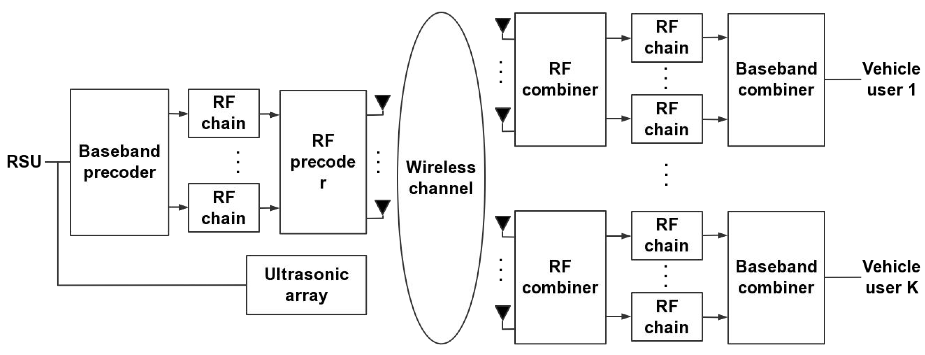
We set up a millimeter-wave massive MIMO communication system operating in the 73 GHz band with a bandwidth of 20 MHz. The number of FFT points is 64, the symbol period is T s = 3 . 2 µs, and the number of subcarriers is 64. A downlink transmission frame structure is used at T 1 = 120 , T 2 = 5 and T 3 = 45 . Other parameters include the expected error ξ = 0.001 , the angular range of AOAs and AODs is [ π / 2 , π / 2 ] , the number of paths is L = 4 , and the maximum Doppler shift is f max .
We consider the performance of the vehicle at two speeds, 90 km/h and 150 km/h. Compare the proposed channel estimation algorithm with the least square (LS), orthogonal matching pursuit (OMP), SBL, and SCPD algorithms. Compare the DOA tracking algorithm with the projection approximation subspace tracking (PAST), projection approximation and subspace tracking of deflation (PASTD), particle filtering (PF), and PF-MUSIC algorithms. We use normalized mean square error (NMSE) to evaluate the estimation accuracy of the channel estimation algorithm and root mean square error (RMSE) to evaluate the tracking accuracy of the DOA tracking algorithm. The expressions for both are as follows:
N M S E = 10 log 10 E H ˜ H F 2 H F 2 ,
R M S E = 1 N R i = 1 N R [ β ^ i ( n ) β ¯ i ( n ) ] 2 ,
where H ˜ denotes the estimated value of the channel, H denotes the actual value of the channel, β ^ i ( n ) denotes the estimated value of the DOA trace in the nth time slot, and β ¯ i denotes the actual value of the DOA.
Figure 4 show the RMSE performance of DOA tracking versus the signal-to-noise ratio (SNR) for vehicle speeds of 90 km/h and 150 km/h. It can be seen that the PAST and PASTD algorithms have larger errors at some estimation points, which is due to the fact that these types of algorithms are based on subspace updates, and it is more difficult to guarantee the orthogonality of the signal and noise subspaces during the update process. The effect of PF class algorithms is better than PAST and PASTD algorithms because the DOA estimates will be closer to the true values due to the multiple iterations of the weights in PF class algorithms. However, the PF algorithm is susceptible to environmental noise. The performance of the PF-MUSIC algorithm is close to that of our proposed algorithm, but the PF-MUSIC algorithm requires a large number of eigenvalue decompositions, which has the problem of high complexity and high computing power. With the increase in vehicle speed, the RMSE performance of various algorithms decreases, i.e., the DOA tracking accuracy decreases, but our algorithm still maintains good RMSE performance. We also compare the DOA single tracking time of different algorithms when the number of array elements is 16, as shown in Table 1. It can be seen that the PF-MUSIC algorithm has a long single tracking time because it takes computational time on the eigenvalue decomposition. The single tracking time of the PF algorithm is slightly shorter than that of the PF-MUSIC algorithm, but it still has a long single tracking time. The single tracking time of the PAST algorithm is close to our proposed algorithm and is faster than that of the PASTD algorithm, which is due to the slower convergence of the PASTD algorithm. Combining the above, the DOA tracking algorithm proposed in this paper has better results than the comparison algorithms.
Figure 5 show the NMSE performance of the channel estimation versus SNR for vehicle speeds at 90 km/h and 150 km/h. It can be seen that the LS algorithm performs poorly in all SNR ranges, especially in the low SNR case, because it does not take into account the noise factor in the channel. It is susceptible to noise. The OMP algorithm performs poorly because it mainly considers quasi-static channels with relatively stable channel conditions and is not applicable to the time-varying channel conditions of V2X. The performance of SBL is also worse but slightly better than that of OMP because SBL considers the sparse characteristics of the channel but not the low-rank characteristics. The SCPD algorithm utilizes the CP tensor decomposition method but does not take into account the effect of the low-rank characteristic. The better NMSE performance of the proposed channel estimation algorithm compared to the comparison algorithm is probably due to the fact that the proposed algorithm combines the DOA tracking algorithm, which accurately updates the beam ground angle information to make the channel conditions more stable, and takes advantage of the low-rank property.
Figure 6 show the bit error rate (BER) versus SNR for channel estimation at vehicle speeds of 90 km/h and 150 km/h. We can see that the BERs of the proposed channel estimation algorithm and the SCPD algorithm are generally lower and better than those of the other compared algorithms, and the BER performance of the proposed channel estimation algorithm is better at higher SNR. The LS algorithm is greatly affected by noise and has a high BER at low SNR. The BER performance of the OMP algorithm is also poorer because we consider the time-varying channel case where the Doppler shift exists and also the speed is higher. The BER performance of the SBL algorithm is slightly better than the OMP, but it does not fully consider the low-rank characteristics and still has some gaps with the proposed channel estimation algorithm.
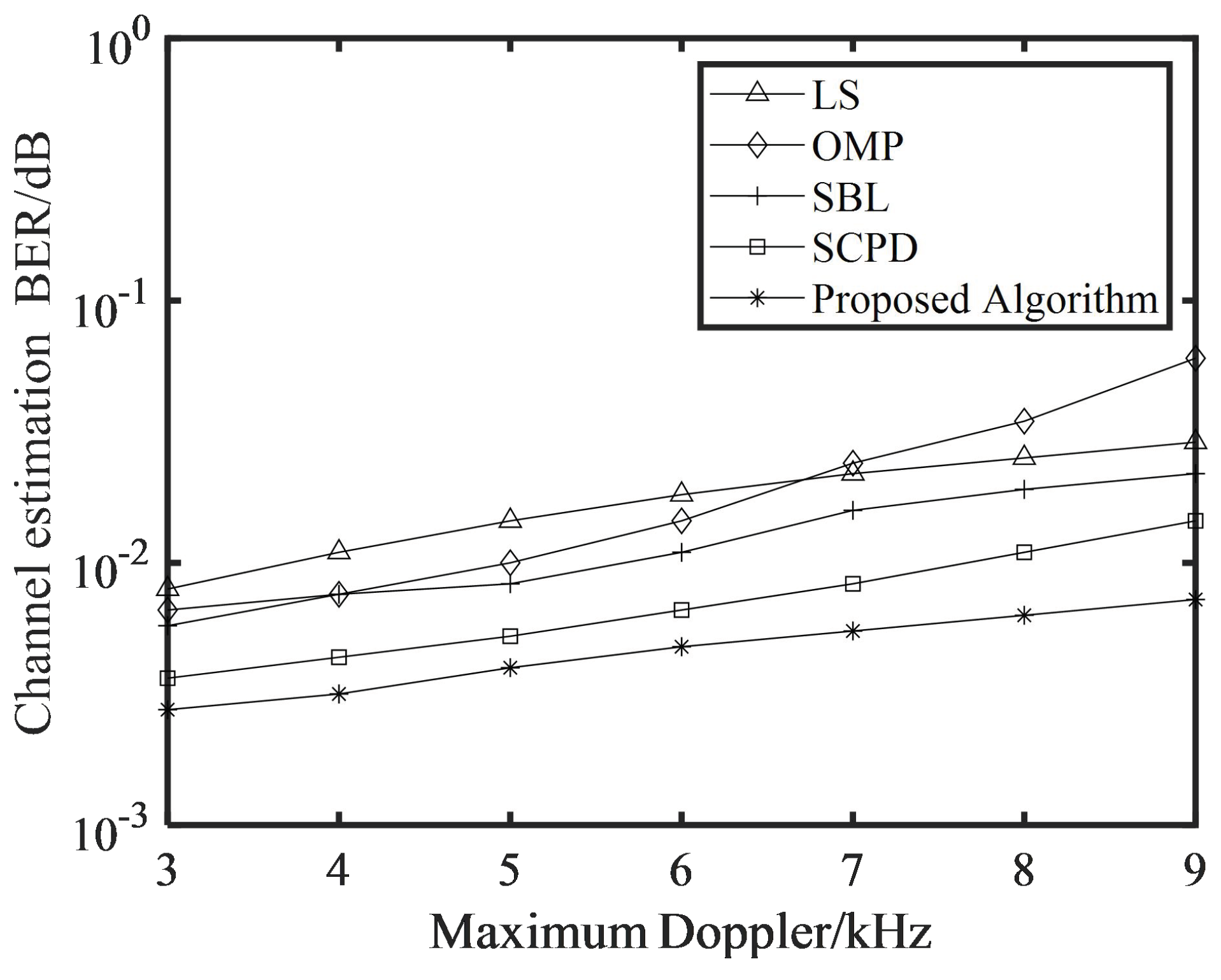
Figure 7 and Figure 8 show the NMSE and BER versus the maximum Doppler shift f max due to the change in vehicle speed, ranging from 3 kHz to 9 kHz. It can be seen that the NMSE and BER performance is related to f max and gradually deteriorates with increasing Doppler shift, which is due to the large Doppler shift when the vehicle speed is high, i.e., corresponding to the channel time-variability enhancement, the channel estimation parameters are not well adapted. However, our proposed scheme still maintains good stability and robustness because it performs DOA tracking and beam angle update compared to the comparison algorithm, and thus is able to sense the channel changes in a more timely manner.

6. Conclusions

In this paper, a set of channel estimation methods for the V2X millimeter wave massive MIMO communication scenario is proposed to solve the problem of rapid channel change due to vehicle movement. First, considering the multidimensional nature of the received signal data, the received signal is represented in tensor form, and the proposed subspace dimensionality reduction tensor decomposition model is used for tensor signal decomposition. The channel estimation process uses a proposed fast-layered alternating iterative tensor algorithm, which performs channel estimation by multiple alternating iterations. In particular, an ultrasonic-aided DOA-tracking method is proposed for the problem of beam direction change due to fast vehicle motion. The method is based on an ultra-high resolution quantization grid and uses the sparse scattering property of ultrasonic waves to transform DOA tracking into a sparse recovery problem. The dictionary matrix can be iteratively and adaptively updated to reduce the effect of quantization errors. The DOA-tracking results can be transformed to obtain a continuously updated communication beam emission direction. Simulation results confirm that the proposed method for estimating V2X fast time-varying channels has better results, and the ultrasonic equipment used is cheaper and more practical. In addition, the channel estimation scheme proposed in this paper can be suitably modified for fast-moving target communication scenarios, such as high-speed railroad communication and low-altitude unmanned aerial vehicle communication, which will help research on channel estimation aspects of these emerging communication scenarios.

Author Contributions

Conceptualization, X.Z. and Z.M.; methodology, X.Z.; software, Z.M. and J.L.; validation, X.Z. and L.Y.; formal analysis, X.Z. and Z.M.; investigation, X.Z. and L.Y.; resources, X.Z. and L.Y.; data curation, J.L.; writing—original draft preparation, Z.M.; writing—review and editing, Z.M.; visualization, J.L.; supervision, X.Z.; project administration, X.Z and J.L. All authors have read and agreed to the published version of the manuscript.

Funding

This research was funded by Shanghai Capacity Building Projects in Local Institutions, grant number 19070502900, Science and Technology Commission of Shanghai Municipality, grant number 22142201900.

Institutional Review Board Statement

Not applicable.

Informed Consent Statement

Not applicable.

Data Availability Statement

Not applicable.

Conflicts of Interest

The authors declare no conflict of interest.

References

  1. Chen, M.; Hwang, K.; Wang, H.; Leung, V.C.; Humar, I. Guest Editorial Special Issue on Internet of Things for Smart Health and Emotion Care. IEEE Internet Things J. 2021, 8, 16718–16722. [Google Scholar]
  2. Lv, Z.; Lou, R.; Singh, A.K. AI empowered communication systems for intelligent transportation systems. IEEE Trans. Intell. Transp. Syst. 2020, 22, 4579–4587. [Google Scholar]
  3. Ridene, S. Mid-infrared emission in InxGa1- xAs/GaAs T-shaped quantum wire lasers and its indium composition dependence. Infrared. Phys. Technol. 2018, 89, 218–222. [Google Scholar]
  4. Mastour, N.; Jemaï, M.; Ridene, S. Calculation of ground state and Hartree energies of MoS2/WSe2 assembled type II quantum well. Micro Nanostruct. 2022, 171, 207417. [Google Scholar] [CrossRef]
  5. Mastour, N.; Ramachandran, K.; Ridene, S.; Daoudi, K.; Gaidi, M. Tailoring the optical band gap of In–Sn–Zn–O (ITZO) nanostructures with co-doping process on ZnO crystal system: An experimental and theoretical validation. Eur. Phys. J. Plus 2022, 137, 1–11. [Google Scholar]
  6. Sakaguchi, K.; Fukatsu, R.; Yu, T.; Fukuda, E.; Mahler, K.; Heath, R.; Fujii, T.; Takahashi, K.; Khoryaev, A.; Nagata, S.; et al. Towards mmwave V2X in 5G and beyond to support automated driving. IEICE Trans. Commun. 2021, 104, 587–603. [Google Scholar] [CrossRef]
  7. Jin, I.G.; Avedisov, S.S.; He, C.R.; Qin, W.B.; Sadeghpour, M.; Orosz, G. Experimental validation of connected automated vehicle design among human-driven vehicles. Transp. Res. Part C Emerg. Technol. 2018, 91, 335–352. [Google Scholar]
  8. Huang, J.; Fang, D.; Qian, Y.; Hu, R.Q. Recent advances and challenges in security and privacy for V2X communications. IEEE Open J. Veh. Technol. 2020, 1, 244–266. [Google Scholar] [CrossRef]
  9. Gyawali, S.; Xu, S.; Qian, Y.; Hu, R.Q. Challenges and solutions for cellular based V2X communications. IEEE Commun. Surv. Tutor. 2020, 23, 222–255. [Google Scholar]
  10. Usman, M.; Qaraqe, M.; Asghar, M.R.; Gebremariam, A.A.; Ansari, I.S.; Granelli, F.; Abbasi, Q.H. A business and legislative perspective of V2X and mobility applications in 5G networks. IEEE Access 2020, 8, 67426–67435. [Google Scholar] [CrossRef]
  11. Naik, G.; Choudhury, B.; Park, J.M. IEEE 802.11 bd & 5G NR V2X: Evolution of radio access technologies for V2X communications. IEEE Access 2019, 7, 70169–70184. [Google Scholar]
  12. Storck, C.R.; Duarte-Figueiredo, F. A survey of 5G technology evolution, standards, and infrastructure associated with vehicle-to-everything communications by internet of vehicles. IEEE Access 2020, 8, 117593–117614. [Google Scholar]
  13. Rappaport, T.S.; Xing, Y.; MacCartney, G.R.; Molisch, A.F.; Mellios, E.; Zhang, J. Overview of millimeter wave communications for fifth-generation (5G) wireless networks—With a focus on propagation models. IEEE Trans. Antennas Propag. 2017, 65, 6213–6230. [Google Scholar] [CrossRef]
  14. Rappaport, T.S.; Sun, S.; Mayzus, R.; Zhao, H.; Azar, Y.; Wang, K.; Wong, G.N.; Schulz, J.K.; Samimi, M.; Gutierrez, F. Millimeter wave mobile communications for 5G cellular: It will work! IEEE Access 2013, 1, 335–349. [Google Scholar]
  15. Pi, Z.; Khan, F. An introduction to millimeter-wave mobile broadband systems. IEEE Commun. Mag. 2011, 49, 101–107. [Google Scholar]
  16. Niu, Y.; Gao, C.; Li, Y.; Su, L.; Jin, D. Exploiting multi-hop relaying to overcome blockage in directional mmwave small cells. J. Commun. Netw. 2016, 18, 364–374. [Google Scholar]
  17. Swindlehurst, A.L.; Ayanoglu, E.; Heydari, P.; Capolino, F. Millimeter-wave massive MIMO: The next wireless revolution? IEEE Commun. Mag. 2014, 52, 56–62. [Google Scholar] [CrossRef]
  18. Long, Y.; Chen, Z.; Fang, J. Minimum number of antennas required to satisfy outage probability in massive MIMO systems. IEEE Wirel. Commun. Lett. 2016, 5, 348–351. [Google Scholar] [CrossRef]
  19. Alsharif, M.H.; Nordin, R. Evolution towards fifth generation (5G) wireless networks: Current trends and challenges in the deployment of millimetre wave, massive MIMO, and small cells. Telecommun. Syst. 2017, 64, 617–637. [Google Scholar]
  20. Ozdemir, Ö.; Anjinappa, C.K.; Hamila, R.; Al-Dhahir, N.; Güvenç, I. Joint frame synchronization and channel estimation: Sparse recovery approach and USRP implementation. IEEE Access 2019, 7, 39041–39053. [Google Scholar] [CrossRef]
  21. Geng, N.; Yuan, X.; Ping, L. Dual-diagonal LMMSE channel estimation for OFDM systems. IEEE Trans. Signal Process. 2012, 60, 4734–4746. [Google Scholar] [CrossRef]
  22. Chen, L.; Liu, A.; Yuan, X. Structured turbo compressed sensing for massive MIMO channel estimation using a Markov prior. IEEE Trans. Veh. Technol. 2017, 67, 4635–4639. [Google Scholar] [CrossRef]
  23. Zhang, R.; Zhao, H.; Zhang, J. Distributed compressed sensing aided sparse channel estimation in FDD massive MIMO system. IEEE Access 2018, 6, 18383–18397. [Google Scholar] [CrossRef]
  24. Chun, C.J.; Kang, J.M.; Kim, I.M. Deep learning-based channel estimation for massive MIMO systems. IEEE Wirel. Commun. Lett. 2019, 8, 1228–1231. [Google Scholar] [CrossRef]
  25. Yang, Y.; Fei, D.; Dang, S. Inter-vehicle cooperation channel estimation for IEEE 802.11 p V2I communications. J. Commun. Netw. 2017, 19, 227–238. [Google Scholar]
  26. Baek, S.; Lee, I.; Song, C. A new data pilot-aided channel estimation scheme for fast time-varying channels in IEEE 802.11 p systems. IEEE Trans. Veh. Technol. 2019, 68, 5169–5172. [Google Scholar] [CrossRef]
  27. Liao, Y.; Hua, Y.; Cai, Y. Deep learning based channel estimation algorithm for fast time-varying MIMO-OFDM systems. IEEE Commun. Lett. 2019, 24, 572–576. [Google Scholar] [CrossRef]
  28. Qin, Q.; Gui, L.; Cheng, P.; Gong, B. Time-varying channel estimation for millimeter wave multiuser MIMO systems. IEEE Trans. Veh. Technol. 2018, 67, 9435–9448. [Google Scholar]
  29. Ma, J.; Zhang, S.; Li, H.; Gao, F.; Han, Z. Time-varying downlink channel tracking for quantized massive MIMO networks. IEEE Trans. Wirel. Commun. 2020, 19, 6721–6736. [Google Scholar]
  30. Zhang, M.; Zhou, X.; Wang, C. Time-varying sparse channel estimation based on adaptive average and MSE optimal threshold in STBC MIMO-OFDM systems. IEEE Access 2020, 8, 177874–177895. [Google Scholar]
  31. Dai, X.; Zhang, H.; Li, D. Linearly time-varying channel estimation for MIMO/OFDM systems using superimposed training. IEEE Trans. Commun. 2010, 58, 681–693. [Google Scholar] [CrossRef]
  32. Huang, S.; Zhang, M.; Gao, Y.; Feng, Z. MIMO radar aided mmwave time-varying channel estimation in MU-MIMO V2X communications. IEEE Trans. Wirel. Commun. 2021, 20, 7581–7594. [Google Scholar] [CrossRef]
  33. Cazzella, L.; Tagliaferri, D.; Mizmizi, M.; Badini, D.; Mazzucco, C.; Matteucci, M.; Spagnolini, U. Deep Learning of Transferable MIMO Channel Modes for 6G V2X Communications. IEEE Trans. Antennas Propag. 2022, 70, 4127–4139. [Google Scholar] [CrossRef]
  34. Mehrabi, M.; Mohammadkarimi, M.; Ardakani, M.; Jing, Y. Decision directed channel estimation based on deep neural network k-step predictor for MIMO communications in 5G. IEEE J. Sel. Areas Commun. 2019, 37, 2443–2456. [Google Scholar]
  35. Shahmansoori, A. Sparse Bayesian multi-task learning of time-varying massive MIMO channels with dynamic filtering. IEEE Wirel. Commun. Lett. 2020, 9, 871–874. [Google Scholar] [CrossRef] [Green Version]
  36. Prasad, R.; Murthy, C.R.; Rao, B.D. Joint channel estimation and data detection in MIMO-OFDM systems: A sparse Bayesian learning approach. IEEE Trans. Signal Process. 2015, 63, 5369–5382. [Google Scholar] [CrossRef]
  37. Araújo, D.C.; De Almeida, A.L.; Da Costa, J.P.; de Sousa, R.T. Tensor-based channel estimation for massive MIMO-OFDM systems. IEEE Access 2019, 7, 42133–42147. [Google Scholar]
  38. Buiquang, C.; Ye, Z. Blind Joint 2-D DOA/Symbols Estimation for 3-D Millimeter Wave Massive MIMO Communication Systems. ACM Trans. Sens. Netw. 2019, 15, 1–24. [Google Scholar] [CrossRef]
  39. Wen, F.; Xu, Y. HOSVD based multidimensional parameter estimation for massive MIMO system from incomplete channel measurements. Multidimens Syst. Signal Process 2018, 29, 1255–1267. [Google Scholar] [CrossRef]
  40. Lin, Y.; Jin, S.; Matthaiou, M.; You, X. Tensor-based channel estimation for millimeter wave MIMO-OFDM with dual-wideband effects. IEEE Trans. Commun. 2020, 68, 4218–4232. [Google Scholar] [CrossRef]
  41. Qin, S.; Zhang, Y.D.; Amin, M.G.; Himed, B. DOA estimation exploiting a uniform linear array with multiple co-prime frequencies. Signal Process. 2017, 130, 37–46. [Google Scholar]
  42. Han, G.; Wan, L.; Shu, L.; Feng, N. Two novel DOA estimation approaches for real-time assistant calibration systems in future vehicle industrial. IEEE Syst. J. 2015, 11, 1361–1372. [Google Scholar] [CrossRef]
  43. Masnadi-Shirazi, A.; Rao, B.D. A covariance-based superpositional CPHD filter for multisource DOA tracking. IEEE Trans. Signal Process. 2017, 66, 309–323. [Google Scholar]
  44. Xin, J.; Sano, A. Efficient subspace-based algorithm for adaptive bearing estimation and tracking. IEEE Trans. Signal Process. 2005, 53, 4485–4505. [Google Scholar]
  45. Chen, H.; Wei, Y.; Bai, Y.; Zhang, X. Sparse recovery for DOA estimation with a reflection path. IEEE Access 2018, 6, 70572–70581. [Google Scholar]
  46. Xie, N.; Guo, W.; Zhang, L.; Wang, H. High resolution DOA estimation method in MIMO radar. Wirel. Pers. Commun. 2016, 91, 219–236. [Google Scholar] [CrossRef]
  47. Li, Y.; Ma, H.; Wu, Y.; Cheng, L.; Yu, D. DOA estimation for echo signals and experimental results in the AM radio-based passive radar. IEEE Access 2018, 6, 73316–73327. [Google Scholar] [CrossRef]
  48. Guo, F.; Liu, H.; Huang, J.; Zhang, X.; Zu, X.; Li, B.; Yuan, X. Design of a direction-of-arrival estimation method used for an automatic bearing tracking system. Sensors 2016, 16, 1145. [Google Scholar] [CrossRef]
  49. Wei, L.; Huang, C.; Alexandropoulos, G.C.; Yuen, C. Parallel factor decomposition channel estimation in RIS-assisted multi-user MISO communication. In Proceedings of the 2020 IEEE 11th Sensor Array and Multichannel Signal Processing Workshop (SAM), Hangzhou, China, 8–11 June 2020; pp. 1–5. [Google Scholar]
Figure 1. Channel hybrid precoding structure for ultrasonic-aided multi-user millimeter-wave massive MIMO system. On the left is the RSU with the wireless communication module and the ultrasonic module, and on the right are the vehicles.
Electronics 11 03742 g001
Figure 2. Subspace dimensionality reduction tensor decomposition model. The process of the first two dimensionality reduction decompositions is used here as an example, and the subsequent decompositions will be performed in the reduced subspace.
Electronics 11 03742 g002
Figure 3. Schematic diagram of the angular transformation of DOA tracking results.
Electronics 11 03742 g003
Figure 4. RMSE performance versus SNR for DOA tracking. Simulation setup: single vehicle; the number of ultrasonic array elements is 16 on the RSU array. (a) The vehicle speed is 90 km/h. (b) The vehicle speed is 150 km/h.
Electronics 11 03742 g004
Figure 5. NMSE performance versus SNR for channel estimation. Simulation setup: single vehicle; the number of transmit antennas N R = 16 , and the transmit RF chains M R = 16 ; the number of receive antennas N V = 4 , and the receive RF chains M V = 4 . (a) The vehicle speed is 90 km/h. (b) The vehicle speed is 150 km/h.
Electronics 11 03742 g005
Figure 6. BER performance versus SNR for channel estimation. Simulation setup: single vehicle; the number of transmit antennas N R = 16 , and the transmit RF chains M R = 16 ; the number of receive antennas N V = 4 , and the receive RF chains M V = 4 . (a) The vehicle speed is 90 km/h. (b) The vehicle speed is 150 km/h.
Electronics 11 03742 g006
Figure 7. NMSE versus maximum Doppler shift f max . Simulation setup: the number of transmit antennas N R = 16 , and the transmit RF chains M R = 16 ; the number of receive antennas N V = 4 , and the receive RF chains M V = 4 .The number of vehicles is 4, and the distance between vehicles is greater than 50 m.
Electronics 11 03742 g007
Figure 8. BER versus maximum Doppler shift f max . Simulation setup: the number of transmit antennas N R = 16 , and the transmit RF chains M R = 16 ; the number of receive antennas N V = 4 , and the receive RF chains M V = 4 .The number of vehicles is 4, and the distance between vehicles is greater than 50 m.
Electronics 11 03742 g008
Table 1. DOA single tracking time for different algorithms when the number of array elements is 16.
AlgorithmDOA Single Tracking Time (s)
PAST0.875
PASTD1.196
PF1.333
PF-MUSIC1.549
Proposed Algorithm0.672
Publisher’s Note: MDPI stays neutral with regard to jurisdictional claims in published maps and institutional affiliations.

