Abstract
Microwave breakdown is crucial to the transmission of high-power microwave (HPM) devices, where a growing number of studies have analyzed the complex interactions between electromagnetic waves and the evolving plasma from theoretical and analytical perspectives. In this paper, we propose a finite-difference time-domain (FDTD) scheme to numerically solve Maxwell’s equation, coupled with a fluid plasma equation for simulating the plasma formation during HPM air breakdown. A subgridding method is adopted to obtain accurate results with lower computational resources. Moreover, the three-dimensional subgridding Maxwell–plasma algorithm is efficiently accelerated by utilizing heterogeneous computing technique based on graphics processing units (GPUs) and multiple central processing units (CPUs), which can be applied as an efficient method for the investigation of the HPM air breakdown phenomena.
1. Introduction
High-power microwave (HPM) systems and devices are widely used in the civilian and military sectors. To better design HPM systems and devices, air breakdown using a HPM source has been extensively investigated and is relatively well understood experimentally [1,2,3,4], as well as theoretically [5,6,7,8,9,10]. In the research on HPM, air breakdown is essential because of the significant limiting factor in the transmission of HPM devices. The transmission capability of a device will be dramatically decreased if the breakdown occurs.
Numerical analyses of microwave breakdown in metallic holes have been well studied. By coupling Maxwell’s equations and a set of electron-fluid model, the effect of air breakdown on intense microwave pulses passing through enclosed aperture holes was studied [11]. A similar conclusion of microwave breakdown in a narrow metallic gap was also obtained theoretically and experimentally in [12]. In [9,10], the FDTD has been adopted to solve a set of coupled Maxwell–plasma problems. Because of the relatively large plasma density gradient during microwave breakdown, the cell size should be small enough to achieve an accurate solution. According to the Courant–Friedrichs–Lewy (CFL) limit, the time step will also be small. As mentioned above, this uniform grid settings hinders the FDTD method from being applied to microwave breakdown problems because of the huge memory requirement and the long execution time. Due to the issues mentioned above, Hamiaz et al. proposed a 2D Maxwell–plasma model based on the finite-volume time-domain (FVTD) scheme, and it is suitable to study microwave breakdown in complex geometries [13]. The results prove that in the plasma region the FVTD method allows for local mesh refinement. A time step of local region used in the FVTD allows for a reduction of the required computational time. In [14,15], the discontinuous Galerkin time-domain (DGTD) [16,17,18] method was proposed for the multiscale and multiphysics modeling and simulation of the HPM breakdown and the Maxwell-plasma interaction. The nodal DGTD method was applied in the solution of the parabolic diffusion equation and the hyperbolic Maxwell’s equations.
In this paper, subgridding FDTD that is accelerated by heterogeneous computing techniques based on GPUs and multiple CPUs is applied to study the air breakdown in HPM devices, which shows significant advantages over conventional FDTD. In the first part of Section 2, the physical model is presented, which is similar to the one used in [19]. The three-dimensional numerical framework is also introduced in this section. In the second part of Section 2, we present the subgridding algorithm and heterogeneous CPU-GPU acceleration to improve computational efficiency and save memory. In Section 3, the subgridding algorithm is used to simulate the air breakdown in the high-power microwave device, which is accelerated by heterogeneous CPU-GPU computing technique. It is found that the simulation results are in good agreement with the experimental results. In Section 4, a discussion on microwave breakdown and acceleration technique is concluded, as an attempt to understand the multiphysics and multiscale problems.
2. Physical and Computation Model
2.1. Physical Model
The physical model adopted in this paper is based on standard Maxwell’s equations linked with a simple plasma diffusion equation [20,21,22,23]. The electromagnetic fields and drive the motion of the plasma charge with electron density , velocity and current density . The physical model is given by
where is the charge of the electron. The ion current density is neglected because it is much smaller compared with the electron current density. In Equation (3), the electron mean velocity is the solution of the simplified momentum equation
where is the electron mass and the is the electron-neutral collision frequency given by
where the is the ambient pressure in Torr. In this paper, Torr. The electron density is governed by a mass conservation equation
where the operator can be reformulated as the sum of two operators
According to [24], the first term on the right () in Equation (7) and the second term on the right () in Equation (6) are insignificant and can be neglected.
The effective diffusion coefficient can be written as a combination of the electron free diffusion coefficient and the ambipolar diffusion coefficient as follows
where
where is the Boltzmann constant, is the electron temperature which can be considered as approximately constant and equal to 2 eV [19], and stands for the electron mobility, which is equal to . The ion mobility is usually supposed to be [24]. The weighting between the free and ambipolar diffusions is adjusted by the unitless factor as
where represents the local dielectric relaxation time.
In Equation (6), the effective ionization frequency usually replaced the combination of attachment frequency and ionization frequency , which can be represented by the electron drift velocity [25,26] as
where is the ionization coefficient and indicated by the following empirical expression
where , , and , is the critical field intensity which determines the proportion of ionization and attachment. The coefficients are , when and , and when [25].
In Equation (13), the effective field represented by
where the mean square root is defined as
We discretized our domain via the Yee grid [27], where the electric fields are collocated with the electron mean velocity in space, the electron density is collocated at the vertices of the Yee grid. The electron velocity and electron density are at the same time step with that of the magnetic fields. The computational grid based on the standard Yee cell is displayed in Figure 1.
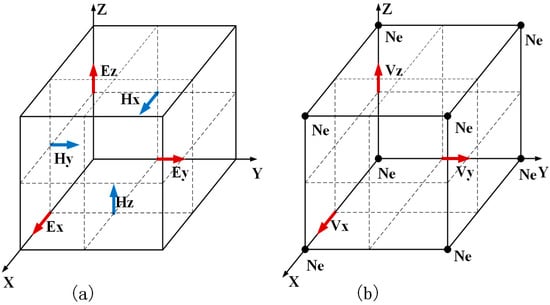
Figure 1.
The Yee grids for the Maxwell–plasma system. (a) Maxwell’s equations. (b) Plasma equations.
Considering the electron mean velocity at , the explicit difference equation for can be deduced as
with
with the central spatial difference and with the explicit time-stepping, the discretized form of Equation (6) is shown as follows:
2.2. Subgridding Algorithm and Heterogeneous CPU-GPU Acceleration
For the traditional FDTD method using the pure dense grid, especially for the simulation of EM interacting with plasmas and targets with delicate structures [28,29,30], the grid size must be small enough to capture the motion of electromagnetic fields and plasma dynamics. However, the fine mesh for simulating plasmas will lead to large memory cost and a long execution time. To solve this problem, the subgridding mesh technique is adopted [31,32,33]. Figure 2 shows the 3-D subgridding interface and the x-component electric field interpolation schematic diagram in the x–z plane. For the sake of simplicity, a grid ratio (GR) of the coarse grid and the dense grid is 3:1 is illustrated. represents the electric fields in the coarse grid and indicates the electric fields and in the dense grid. There are three different interpolation types in Figure 2. and belong to type one, in which the coarse grid electric fields overlap with dense grid electric fields, and these electric fields can be directly obtained from coarse grid electric fields. , , and belong to type two, in which these electric fields can be obtained with the linear interpolation method using the coarse grid electric fields. , , , , and belong to type three, in which these electric fields can be obtained with the linear interpolation method using the dense grid electric fields. The coefficients are displayed in Figure 2b.
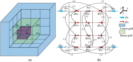
Figure 2.
(a) The subgridding interface in three dimensions and (b) the x-component electric field interpolation schematic diagram in the x–z plane.
The update equations for coarse grid electric fields in the coarse grid region, such as and , are those of the standard FDTD. The update equation for coarse grid electric fields at the interface, such as , , and , is given by
where is the grid ratio and are the magnetic fields in the dense grid region. There are four types of dense grid magnetic fields at the interface, as shown in Figure 3. Most of the dense grid magnetic fields belong to the type in Figure 3a, in which the electric field is at the middle of the interface and the magnetic fields are all in the dense grid region. In Figure 3b, the electric field is parallel to the boundary of the interface and there are dense magnetic fields in x-direction, but only in the z-direction. In Figure 3c, the electric field is perpendicular to the boundary of the interface and there are dense magnetic fields in the z-direction, but only in the x-direction. In Figure 3d, the electric field is perpendicular to one boundary of interface and parallel to another boundary of the interface, where there are dense magnetic fields in the z-direction and in the x-direction.
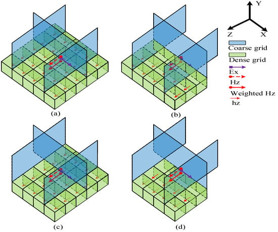
Figure 3.
3-D subgridding interface and weighted magnetic field, where (a) is at the middle of the interface, (b) is parallel to the boundary of the interface, (c) is perpendicular to the boundary of the interface, and (d) is perpendicular to one boundary of the interface and parallel to another boundary of the interface.
The coefficient matrix in Equation (19) has different four expressions which correspond to four different situations in Figure 3.
| (a) | (b) | |
| (c) | (d) |
The other five interfaces follow the same linear interpolation method. The subgridding algorithm, with different GR values, which are equal to 5, 7, and 9 are also employed in Maxwell–plasma equations in this paper.
Generally, a dense mesh and coarse mesh are adopted for updating plasmas and low refractive index media, respectively. As a rule-of-thumb, the dense/coarse grid size should be set to at least 200/10 cells per wavelength for the plasma and dielectrics. To efficiently execute the FDTD code, we used a heterogeneous computing technique. An example of a heterogeneous computing platform is shown in Figure 4, containing at least one multicore CPU and one or more GPUs. For the computation of EM fields in coarse grid regions, the CPU is employed, whereas the GPU is employed for the computation of EM fields and physical fields within dense grid regions. The PCI-e port connects the GPUs with the host. Different programming models and vendor-specific techniques are incorporated into this system to ensure cross-device execution of applications. In addition, this system provides kernel launch control, automatic data communication mechanisms, and memory management of devices. A GPU is well suited to parallel computation due to its Compute Unified Device Architecture (CUDA), which provides an interface for multiple languages and is compatible with several compilers. An abstracted representation of the GPU’s hard resources is called a 3-D grid, whose basic unit is called a block. The block is a 3-D structure made up of threads, which constitute its basic unit. In parallel programs, the scheduler assigns tasks within a block to a stream multiprocessor (SM), with each SM handling multiple blocks simultaneously.
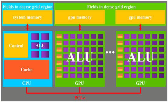
Figure 4.
Heterogeneous computing platform.
In this paper, there are two types of parallelism, one is the coarse-grained parallelism and the other is the fine-grained parallelism. In a heterogeneous system, the parallelism between CPUs and GPU is coarse-grained parallelism. This type of parallelism is achieved by arranging the coarse grid electric fields and magnetic fields in CPUs and arranging the dense grid electric fields, magnetic fields, electron density, and velocity in GPUs. The parallelism between threads is fine-grained parallelism. As shown in Figure 5, the FDTD grid is decomposed and allocated to the different processor units (PUs) in the heterogeneous system. Consequently, the components on the truncated boundary, as well as those involved in their updated equation, are not involved in the same processor. Data communication between adjacent processors is necessary after each iteration. In this paper, there is an imaginary buffer established between the two processors. After the electric field on the truncated of CPU is updated at each time step, obtained by interpolation method from coarse grid is transferred to the imaginary buffer for updating the magnetic field on the truncated of GPU in the next time. Similarly, after the magnetic on the truncated of GPU is updated at each time step, obtained by weighted summation method from dense grid is transferred to the imaginary buffer for updating the electric field on the truncated of the CPU in the next time.
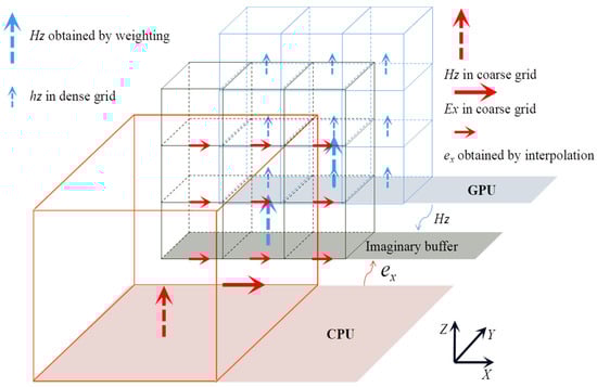
Figure 5.
Data exchange between the CPU and GPU.
3. Results
In this section, we apply the subgridding algorithm to simulate the air breakdown in the high-power microwave device. As shown in inset of Figure 6, the solution domain is an infinite wall with periodic PEC apertures, where the thickness is 0.3 mm, the length is 5 mm, and the width is 1.2 mm. A sinusoidal temporal profile plane wave polarized in the z-direction with a central frequency of 25 GHz and amplitude of 2 MV/m is launched at the TF/SF boundary and propagates toward the y-direction. The y-direction is truncated using the PMLs, and periodic boundary conditions are used in x- and z-direction. The initial electron density is assumed to be uniform (equal to ) in the aperture region at standard atmospheric pressure. The computational domain, including the metallic aperture, is meshed by dense grids and sandwiched by two coarse mesh regions for free-space domains.
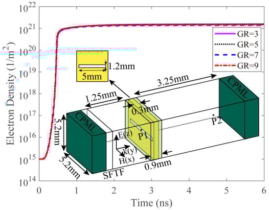
Figure 6.
Temporal evolution of the electron density recorded at P1 for different GRs and the illustration of the solution domain of the microwave breakdown problem.
In Figure 6, we plot the evolvement of the plasma density at P1 for different GR. The electron density increases exponentially from its initial value of to over within the first 0.5 nanoseconds, indicating that the electron density is increasing massively from its initial value and then maintains s steady state. For different GRs, the results are in good agreement.
We recorded the component at points P1 (the center of aperture) and P2 (the distance between P1 and P2 is 2.81 mm). Figure 7 shows the temporal waveform of the electric fields recorded at P1 and P2 for GR = 3, 5, 7 and 9. The results are consistent with the results in [13]. From Figure 7, one can see that the electric field at P1 increases initially due to the field confinement of the metallic aperture. While the electric field magnitude rises above the breakdown threshold, the electric field magnitude dramatically decreases. The temporal profile of the electric field at P2 also demonstrates a similar result after the air breakdown; that is, the existence of plasma hinders the field transmission. Moreover, relative errors in dB at P2 are also shown in Figure 7. For different GR, there are maximum relative errors when the air starts ionizing. After 0.5 ns, the relative error is at much lower values.
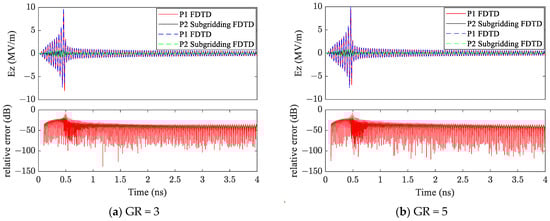
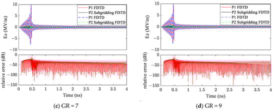
Figure 7.
Temporal response of the component recorded at P1 and P2 for different GR.
To acquire a deep understanding of the physical process and compare the results between the dense grid and subgrid, the spatial and temporal evolution of the effective field is presented in Figure 8, where (a), (b), (c), (d), and (e) represent the field distributions at 0.01 ns, 0.36 ns, 0.42 ns, 0.45 ns, and 0.1 ns, respectively. At 0.01 ns, due to the edge effect, the electric field at the aperture edge begins to increase, leading to the ionization of air. Within a short period, electron density increases dramatically. Then, the plasma formed by ionization will further cause electric field enhancement around the plasma. This process is shown in Figure 8b,c. In Figure 8d, the center of the aperture reaches the maximum value, the air in the center of the aperture also starts ionizing. After ionization of the entire aperture is completed, the plasma hinders the propagation of electromagnetic waves, as shown in Figure 8e.
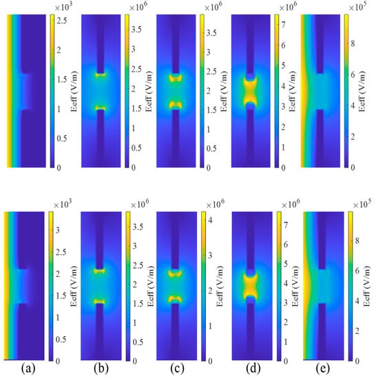
Figure 8.
The time evolution of the effective electric field in the y–z plane in the dense grid (upper panel) and subgrid (lower panel) at (a) 0.01 ns, (b) 0.36 ns, (c) 0.42 ns, (d) 0.45 ns, and (e) 0.1 ns.
To validate our subgridding FDTD method and benchmark the speed of the CPU/GPU heterogeneous computing technique, the proposed method was compared with a conventional FDTD CPU where serial code was running. The CPU used here was an Intel Core i9-10900K @ 3.70 GHz. The GPU used was a NVIDIA GeForce RTX 3090. The required memory and simulation time for different GRs are listed in Table 1. Compared with conventional FDTD, the subgridding FDTD accelerated by the heterogeneous computing technique shows noticeable computation time and memory savings.

Table 1.
Memory ratio and speedup in conventional FDTD (CPU) and subgridding FDTD (CPU-GPU) for different grid ratio.
4. Conclusions
In this paper, A 3-D Maxwell–plasma model based on a subgridding FDTD algorithm has been developed and accelerated with the CPU/GPU heterogeneous computing technique. The results demonstrate that the subgridding FDTD can use less memory and requires a shorter time to obtain the same precision as the conventional FDTD method. For the subgridding FDTD, a smaller grid can get more accurate results. According to the CFL condition, the timestep should be pretty small, leading to a long simulation time. We used the CPU/GPU heterogeneous computing technique to accelerate this algorithm, and the results show that the proposed heterogeneous computing technique can effectively improve the simulation efficiency. The algorithm will be helpful for multiphysics and multiscale problems.
Author Contributions
Conceptualization, J.F.; methodology, J.F.; software, W.C.; validation, M.F.; formal analysis, J.F.; investigation, M.F.; resources, X.W.; data curation, K.S.; writing—original draft preparation, J.F. and M.F.; writing—review and editing, Z.H. and X.W.; visualization, G.X.; supervision, Z.H. and X.W.; project administration, M.F.; funding acquisition, X.W. All authors have read and agreed to the published version of the manuscript.
Funding
This work was funded by the National Science Foundation of China (NSFC) (Nos. 61901001, 61901004, U20A20164), Anhui Province (No. 1908085QF259, No. GXXT-2021-027), State Key Laboratory of Millimeter Waves, Southeast University (K202230).
Data Availability Statement
All the calculation results and relevant data are from our own innovative work, parts of the data that are adopted in our work have already quoted and listed in the references.
Conflicts of Interest
The authors declare no conflict of interest.
References
- McDonald, A.D. Microwave Breakdown in Gases; Wiley Publisher: New York, NY, USA, 1966. [Google Scholar]
- Stefan, B.; Kleine, H.; O’Byrne, S. On the measurement of laser-induced plasma breakdown thresholds. J. Appl. Phys. 2013, 114, 093101. [Google Scholar]
- Hidaka, Y.; Choi, E.; Mastovsky, I.; Shapiro, M.A.; Sirigiri, J.R.; Temkin, R.J.; Edmiston, G.F.; Neuber, A.A.; Oda, Y. Plasma structures observed in gas breakdown using a 1.5 MW, 110 GHz pulsed gyrotron. Phys. Plasmas 2009, 16, 055702. [Google Scholar] [CrossRef]
- Cook, A.M.; Shapiro, M.A.; Temkin, R.J. Pressure dependence of plasma structure in microwave gas breakdown at 110 GHz. Appl. Phys. Lett. 2010, 97, 011504. [Google Scholar] [CrossRef]
- Nam, S.K.; Verboncoeur, J.P. Theory of filamentary plasma array formation in microwave breakdown at near-atmospheric pressure. Phys. Rev. Lett. 2009, 103, 055004. [Google Scholar] [CrossRef] [PubMed]
- Boeuf, J.P.; Chaudhury, B.; Zhu, G.Q. Theory and modeling of self-organization and propagation of filamentary plasma arrays in microwave breakdown at atmospheric pressure. Phys. Rev. Lett. 2010, 104, 015002. [Google Scholar] [CrossRef]
- Anderson, D.; Lisak, M.; Lewin, T. Breakdown in air-filled microwave waveguides during pulsed operation. J. Appl. Phys. 1984, 56, 1414–1419. [Google Scholar] [CrossRef]
- Zhao, P.; Guo, L.; Shu, P. Interaction of high-power microwave with air breakdown plasma at low pressure. Phys. Plasmas 2016, 23, 092105. [Google Scholar] [CrossRef]
- Arcese, E.; Rogier, F.; Boeuf, J.P. Plasma fluid modeling of microwave streamers: Approximations and accuracy. Phys. Plasmas 2017, 24, 113517. [Google Scholar] [CrossRef]
- Hamiaz, A.; Ferrières, X.; Pascal, O. Efficient numerical algorithm to simulate a 3D coupled Maxwell–plasma problem. Math. Comput. Simul. 2020, 174, 19–31. [Google Scholar] [CrossRef]
- Sieger, G.E.; Lee, J.; Mayhall, D.J. Computer simulation of nonlinear coupling of high-power microwaves with slots. IEEE Trans. Plasma Sci. 1989, 17, 616–621. [Google Scholar] [CrossRef]
- Jordan, U.; Anderson, D.; Backstrom, M.; Kim, A.V.; Lisak, M.; Lundén, O. Microwave breakdown in slots. IEEE Trans. Plasma Sci. 2004, 32, 2250–2262. [Google Scholar] [CrossRef]
- Hamiaz, A.; Klein, R.; Ferrieres, X.; Pascal, O.; Boeuf, J.P.; Poirier, J.R. Finite volume time domain modelling of microwave breakdown and plasma formation in a metallic aperture. Comput. Phys. Commun. 2012, 183, 1634–1640. [Google Scholar] [CrossRef]
- Yan, S.; Greenwood, A.D.; Jin, J.M. Modeling of plasma formation during high-power microwave breakdown in air using the discontinuous Galerkin time-domain method. IEEE J. Multiscale Multiphys. Comput. Tech. 2016, 1, 2–13. [Google Scholar] [CrossRef]
- Yan, S.; Greenwood, A.D.; Jin, J.M. Simulation of High-Power Microwave Air Breakdown Modeled by a Coupled Maxwell–Euler System with a Non-Maxwellian EEDF. IEEE Trans. Antennas Propag. 2018, 66, 1882–1893. [Google Scholar] [CrossRef]
- Chen, J.; Liu, Q.H.; Chai, M.; Mix, J.A. A non-spurious 3-D vector discontinuous Galerkin finite-element time-domain method. IEEE Microw. Wirel. Compon. Lett. 2009, 20, 1–3. [Google Scholar] [CrossRef]
- Tobón, L.E.; Ren, Q.; Liu, Q.H. A new efficient 3D discontinuous Galerkin time domain method for large and multiscale electromagnetic simulations. J. Comput. Phys. 2015, 283, 374–387. [Google Scholar] [CrossRef]
- Ren, Q.; Tobón, L.E.; Sun, Q.; Liu, Q.H. A new 3-D nonspurious discontinuous Galerkin spectral element time-domain (DG-SETD) method for Maxwell’s equations. IEEE Trans. Antennas Propag. 2015, 63, 2585–2594. [Google Scholar] [CrossRef]
- Kourtzanidis, K.; Boeuf, J.; Rogier, F. Three dimensional simulations of pattern formation during high-pressure, freely localized microwave breakdown in air. Phys. Plasmas 2014, 21, 123513. [Google Scholar] [CrossRef]
- Chaudhury, B.; Boeuf, J.P. Computational Studies of Filamentary Pattern Formation in a High Power Microwave Breakdown Generated Air Plasma. IEEE Trans. Plasma Sci. 2010, 38, 2281–2288. [Google Scholar] [CrossRef]
- Chaudhury, B.; Boeuf, J.P.; Zhu, G.Q.; Pascal, O. Physics and modelling of microwave streamers at atmospheric pressure. J. Appl. Phys. 2011, 110, 113306. [Google Scholar] [CrossRef]
- Fang, M.; Huang, Z.; Sha, W.E.; Xiong, X.Y.; Wu, X. Full hydrodynamic model of nonlinear electromagnetic response in metallic metamaterials. Prog. Electromagn. Res. 2016, 157, 63–78. [Google Scholar] [CrossRef]
- Fang, M.; Shen, N.H.; Wei, E.; Huang, Z.; Koschny, T.; Soukoulis, C.M. Nonlinearity in the Dark: Broadband Terahertz Generation with Extremely High Efficiency. Phys. Rev. Lett. 2019, 122, 027401. [Google Scholar] [CrossRef] [PubMed]
- Zhu, G.Q.; Boeuf, J.P.; Chaudhury, B. Ionization–diffusion plasma front propagation in a microwave field. Plasma Sources Sci. Technol. 2011, 20, 035007. [Google Scholar] [CrossRef]
- Raizer, Y.P. Gas Discharge Physics; Springer: Berlin, Germany, 1991. [Google Scholar]
- Warne, L.K.; Jorgenson, R.E.; Nicolaysen, S.D. Ionization Coefficient Approach to Modeling Breakdown in Nonuniform Geometries; Sandia Report SAND2003-4078; Sandia National Laboratories (SNL): Albuquerque, NM, USA; Livermore, CA, USA, 2003. [Google Scholar]
- Yee, K. Numerical solution of initial boundary value problems involving maxwell’s equations in isotropic media. IEEE Trans. Antennas Propag. 1966, 14, 302–307. [Google Scholar]
- Kumar, A.; Althuwayb, A.A.; Chaturvedi, D.; Kumar, R.; Ahmadfard, F. Compact planar magneto-electric dipole-like circularly polarized antenna. IET Commun. 2022, 1–6. [Google Scholar] [CrossRef]
- Kumar, R.; Thummaluru, S.R.; Chaudhary, R.K. Improvements in Wi-MAX reception: A new dual-mode wideband circularly polarized dielectric resonator antenna. IEEE Antennas Propag. Mag. 2019, 61, 41–49. [Google Scholar] [CrossRef]
- Chandra, A.; Mishra, N.; Kumar, R.; Kumar, K.; Patil, H.Y. A superstrate and FSS embedded dual band waveguide aperture array with improved far-field characteristics. Microw. Opt. Technol. Lett. 2022, 1–7. [Google Scholar] [CrossRef]
- Xiao, K.; Pommerenke, D.J.; Drewniak, J.L. A three-dimensional FDTD subgridding algorithm based on interpolation of current density. IEEE Trans. Antennas Propag. 2007, 55, 1981–1990. [Google Scholar] [CrossRef]
- Chang, C.; Sarris, C.D. An efficient implementation of a 3D spatially-filtered FDTD subgridding scheme. IEEE Int. Symp. Antennas Propag. 2012, 1–2. [Google Scholar] [CrossRef]
- Bérenger, J. A Huygens subgridding for the FDTD method. IEEE Trans. Antennas Propag. 2006, 54, 3797. [Google Scholar]
Publisher’s Note: MDPI stays neutral with regard to jurisdictional claims in published maps and institutional affiliations. |
© 2022 by the authors. Licensee MDPI, Basel, Switzerland. This article is an open access article distributed under the terms and conditions of the Creative Commons Attribution (CC BY) license (https://creativecommons.org/licenses/by/4.0/).