Autonomous Air Combat Maneuvering Decision Method of UCAV Based on LSHADE-TSO-MPC under Enemy Trajectory Prediction

Abstract

In this paper, an autonomous UCAV air combat maneuvering decision method based on LSHADE-TSO optimization in a model predictive control framework is proposed, along with enemy trajectory prediction. First, a sliding window recursive prediction method for multi-step enemy trajectory prediction using a Bi-LSTM network is proposed. Second, Model Predictive Control (MPC) theory is introduced, and when combined with enemy trajectory prediction, a UCAV maneuver decision model based on the MPC framework is proposed. The LSHADE-TSO algorithm is proposed by combining the LSHADE and TSO algorithms, which overcomes the problem of traditional sequential quadratic programming falling into local optimum when solving complex nonlinear models. The LSHADE-TSO-MPC air combat maneuver decision method is then proposed, which combines the LSHADE-TSO algorithm with the MPC framework and employs the LSHADE-TSO algorithm as the optimal control sequence solver. To validate the effectiveness of the maneuvering decision method proposed in this paper, it is tested against the test maneuver and the LSHADE-TSO decision algorithm, respectively, and the experimental results show that the maneuvering decision method proposed in this paper can beat the opponent and win the air combat using the same weapons and flight platform. Finally, to demonstrate that LSHADE-TSO can better exploit the decision-making ability of the MPC model, LSHADE-TSO is compared to various optimization algorithms based on the MPC model, and the results show that LSHADE-TSO-MPC can not only help obtain air combat victory faster but also demonstrates better decision-making ability.

1. Introduction

Countries all over the world are accelerating the development of unmanned combat aerial vehicles (UCAVs) as artificial intelligence technology advances [1]. AlphaDogfight, a DARPA-sponsored proximity autonomous intelligent air warfare project in the United States, exemplifies the most recent application of artificial intelligence in the field of autonomous air combat [2]. However, the current level of intelligence is insufficient to meet the actual needs, so UCAV autonomous air warfare has been studied as an important issue [3,4].

According to the OODA ring [5], decision making is the central component of UCAV autonomous air combat, serving as the “brain” of the UCAV [6]. Current close air combat maneuver decision methods are classified into three types [7]: game theory-based maneuver decision methods, artificial intelligence-based maneuver decision methods, and optimization theory-based methods.

The game theory-based maneuver decision method mainly employs game theory for air combat maneuver decisions, and it consists mainly of the differential countermeasure method and the influence diagram method. The differential countermeasure method is used to solve bilateral extreme value problems by converting offensive and defensive countermeasures. In Ref. [8], Lee et al. used a game-theoretic-based minmax algorithm to select the optimal maneuver command by constructing a score matrix, and the simulation results showed that it could make fast decisions; discrete maneuvers are used in the library text, which may result in the maneuvers obtained from the decision not being the globally optimal maneuver strategy. The influence diagram method uses expert knowledge from air combat games and is a decision model with a directed acyclic graph representation. Virtanen et al. [9] describe a multi-stage influence diagram game that simulates maneuvering decisions in one-to-one air combat and determines and achieves a Nash equilibrium of the dynamic game at each decision segment, but the influence diagram approach is complex and difficult to satisfy in real time.

Artificial intelligence-based maneuvering decision methods mainly include rule-based expert system methods and deep neural network-based reinforcement learning methods, etc. The rule-based expert system approach is an expert system library built according to IF-THEN rules, and the corresponding maneuvers are performed when the rules are met. Fu Li et al. [10] combined expert systems with rolling time-domain optimization, and used a rolling time-domain optimal control model when the expert system failed, which can make decisions quickly and effectively, but it is difficult to improve the rule base establishment of the expert system. Unlike expert systems, deep neural network-based reinforcement learning methods do not require air combat samples and enable autonomous air combat maneuvering decisions through self-learning and self-updating. Yang et al. [11] established a maneuver decision model based on Deep Q Network (DQN) and achieved autonomous maneuver decisions against enemy close range after phased training, but the reinforcement learning method has long training time and the effect is difficult to guarantee. Jiseon et al. [12] use reinforcement learning on multi-UAV target tracking. Their improved algorithm has the potential to be applied to the multi-UAV air combat problem.

Optimization theory-based methods primarily convert maneuver decision problems into single-objective or multi-objective optimization problems and solve them using heuristic optimization algorithms. Ruan et al. [13] used the Transfer Learning Pigeon-Inspired Optimization (TLPIO) algorithm to search for optimal hybrid strategies and verify the search accuracy of the algorithm using a test function, but the paper does not compare the algorithm with other heuristics on the maneuver decision problem. It does not show the advantage of the algorithm for the maneuvering decision problem. Yang et al. [14] designed an autonomous evasive maneuver decision method for over-the-horizon air combat, considering both longer off-target distance, less energy consumption, and longer maneuver duration, and transformed the evasive maneuver problem into a multi-objective optimization problem. A hierarchical multi-objective evolutionary algorithm (HMOEA) has been designed to find the approximate Pareto optimal solution of the problem. Simulation results showed that it can meet the needs of the different evasive tactics of UCAV. However, this method can only be used for escape, not for attack. Li et al. [15] proposed a multi-UCAV over-the-horizon cooperative occupancy maneuver decision method, which uses weapon strike zones and air combat geometry to establish dominance functions for posture evaluation. The multi-UCAV maneuver decision problem was transformed into a mixed integer nonlinear programming (MINLP) problem and was solved using an improved discrete particle swarm optimization (DPSO) algorithm. There is also no comparison of the effectiveness of different algorithms on the maneuvering decision problem in the paper.

By categorizing the existing researchs,

Table 1. Overview of close air combat maneuver decision methods.

Maneuver Decision Methods	Specific Methods	Literature
Game theory-based maneuver decision methods	Differential countermeasure method	[8,16,17]
	The influence diagram method	[9,18,19]
Artificial intelligence-based maneuver decision methods	Rule-based expert system methods	[9,20,21]
	Deep neural network-based reinforcement learning methods	[11,22,23]
Optimization theory-based methods	Single-objective optimization	[13,15,24]
	Multi-objective optimization	[14,25,26]

was obtained. According to the findings of the preceding research, it is difficult to find an analytical solution to achieve Nash equilibrium in the real air combat environment using the maneuvering decision method based on game theory, and the high computational complexity makes meeting the real-time requirements difficult. The air combat rules are tough to complete using the artificial intelligence-based maneuvering method, and the effect of using reinforcement learning requires a significant amount of training time. The maneuvering decision method based on optimization theory typically establishes the situation function and solves the control variables by the method of situation finding, which easily falls into the local optimum. Additionally, the decision dimension is low when solved using a heuristic algorithm, making it difficult to realize its advantages.

Additionally, none of the studies mentioned above used the enemy aircraft’s predicted trajectory to guide their maneuvering decisions or took into account how they would situate themselves over a longer period of time. When establishing the objective function, the next moment’s posture advantage of our aircraft is considered, and the UCAV can only maintain the posture advantage from time to time, which is easily deceived by the enemy tactics.

There are various control methods currently available for UAVs, which have been developed to meet the needs of trajectory tracking [27] and geographic boundary avoidance [28]. However, for the air combat environment, open-loop system control methods such as model predictive control are still used as the classical control methods [29].

Therefore, this paper adopts a model predictive control framework that combines trajectory prediction of enemy aircraft with the average of the relative situations of our aircraft and enemy aircraft at multiple future moments as the objective function. Multiple steps are taken in one decision, and the first step is used as the input for the next moment, thus completing the maneuver decision and realizing the utilization of enemy aircraft trajectory prediction data and the consideration of the long-term situation. Compared with the existing work, this paper is able to break through the problem that optimization algorithms for maneuvering decision problems tend to fall into local optimality and uses the MPC framework to incorporate trajectory prediction into maneuvering decisions. It aims to obtain air combat victory faster. Most importantly, the paper compares the different algorithms used for maneuvering decisions. The innovation and main work of this paper are shown below:

(1)

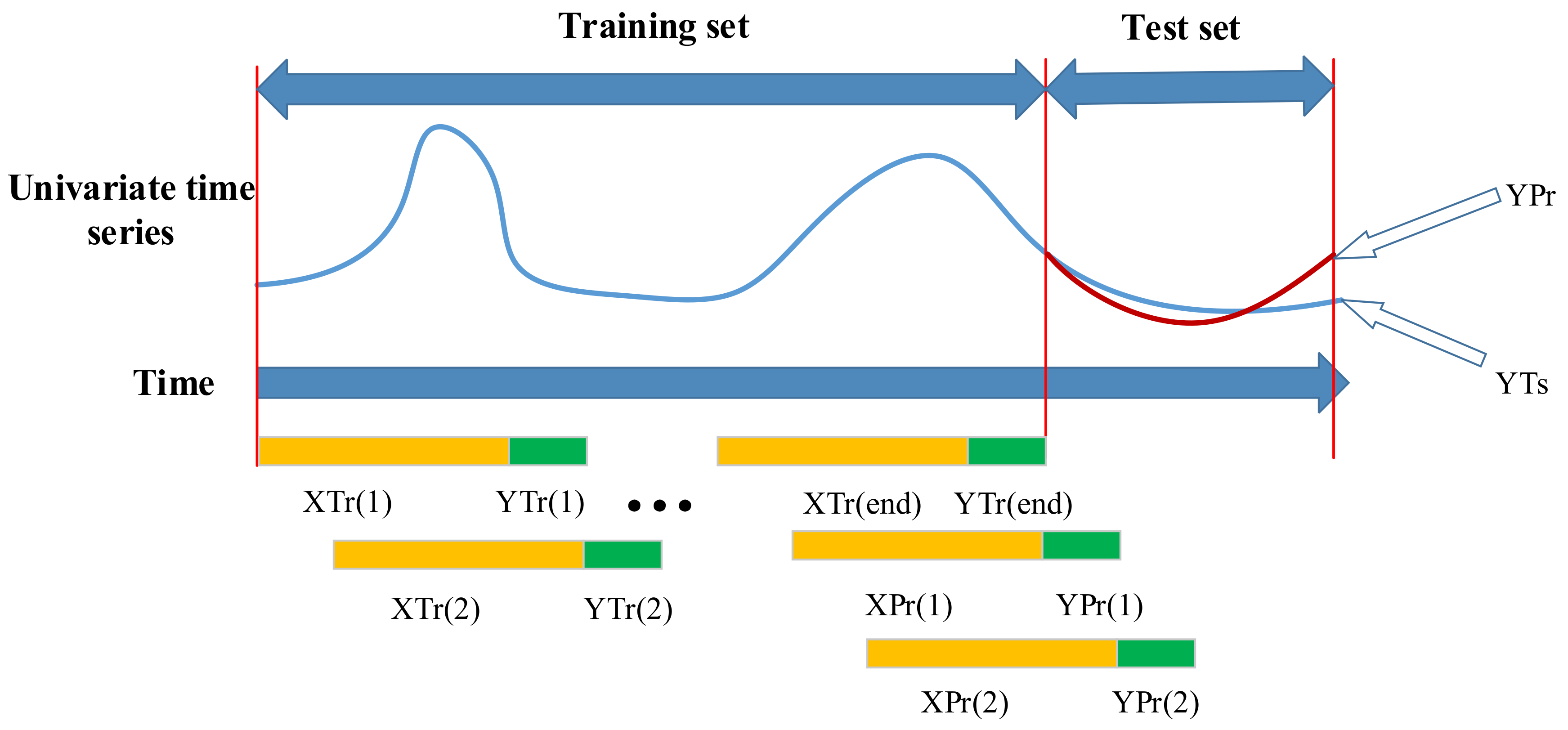
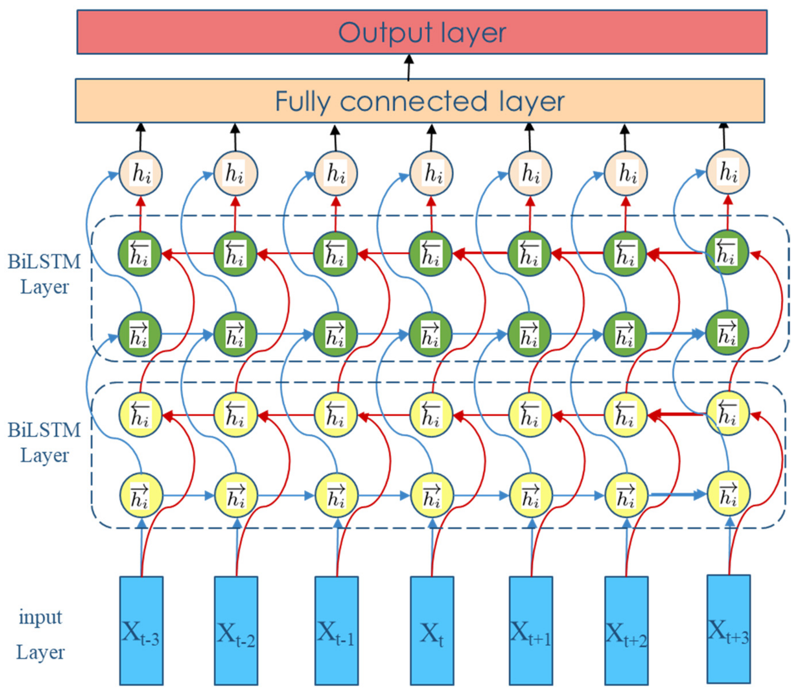
For long-time domain time series data prediction, Bi-LSTM network rolling recursive prediction theory is introduced, which solves the short time domain for the trajectory prediction issue.

(2)

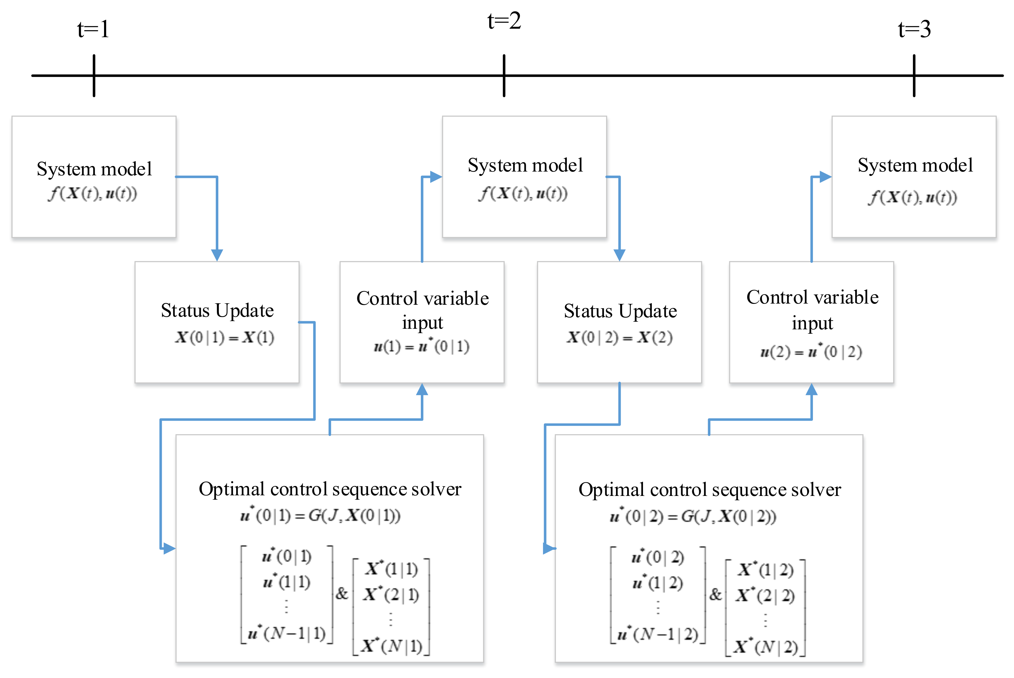
A model predictive control theory is presented, which combines a target prediction trajectory with several steps in a single decision, using the control variable from the first control sequence as the control variable for the next instant. Future dynamics are incorporated into the objective function using this method.

(3)

The LSHADE-TSO algorithm replaces the traditional model predictive control solver, sequential quadratic programming, which solves the problem of complex nonlinear models easily falling into local optimum.

(4)

Based on a modification of the LSAHDE algorithm, the LSHADE-TSO algorithm is proposed, and the search accuracy is validated using the CEC2014 test functions.

(5)

The superiority of the maneuvering decision method proposed in this paper is demonstrated by an experimental analysis of air combat countermeasures, and the decision duration is examined to demonstrate that it can meet real-time demand.

The rest of the paper is organized as follows. Multi-step trajectory prediction based on a Bi-LSTM network is described in Section 2. Section 3 describes the UCAV maneuvering decision model in the MPC framework; it combines the trajectory prediction and MPC framework for maneuvering decisions. The close air combat situation function is also presented in Section 3. In Section 4, the LSHADE-TSO algorithm is proposed and tested by CEC2014 test functions. Section 5 demonstrates simulation results for the comparison of different maneuvering decision methods and algorithms. Section 6 summarizes the simulation results and the work in this paper.

2. Multi-Step Trajectory Prediction Based on a Bi-LSTM Network

2.1. Sliding-Window Recursive Prediction

From the literature [30], it is known that the 3D coordinate independent prediction converges faster and has higher accuracy than the overall prediction, so this paper adopts the single sequence multi-step prediction method to predict the future trajectory of the enemy.

The time series prediction problem is the prediction of unknown future states, but in one part of the study, the sliding window is constructed using the actual values on the prediction of the test set [31], which is equivalent to leaking the test set data that must be predicted in advance, and there is actually a time paradox, so this paper adopts the method of constructing the sliding window using the predicted values, as shown in the figure below:

In Figure 1, the whole single variable time series is divided into training set and test set, and in the training set, the last position of the time window is used as the response for rolling training. In the test set, the entire test set is set as unknown, and the end of the training set is used as the input to predict the first datapoint, YPr(1), of the test set, and then YPr(1) and the end of the training set are reorganized into XPr(2) to predict the next point, YPr(2). This rolling cycle continues to achieve multi-step prediction of the target trajectory and output YPr.

2.2. Bi-LSTM Network

The gate structure in LSTM includes input gate, output gate, and forgetting gate. They are calculated as follows.

$$\mathrm{forgetting} \mathrm{gate}: F_t = \sigma (W_{f}g[h_{t-1},X_t] + b_f)$$

(1)

$$\mathrm{input} \mathrm{gate}: i_t = \sigma (W_{i}g[h_{t-1},X_t] + b_i)\cdot tanh(W_{c}g[h_{t-1},X_t] + b_c)$$

(2)

$$\mathrm{output} \mathrm{gate}: O_t = \sigma (W_{o}g[h_{t-1},X_t] + b_o)$$

(3)

$$h_t = O_t·tanh(C_t)$$

(4)

where, $W_f$, $W_i$, $W_c$, and $W_o$ are the coefficient matrix; $b_f$, $b_i$, $b_c$, and $b_o$ are the bias matrix; $\sigma$ represents a sigmoid activation function; $F_t$ represents the forget gate; $i_t$ represents the input gate; $O_t$ represents the output gate; $h_{t-1}$ represents the output of the previous unit; and $h_t$ represents the output of the current unit. The forgetting gate determines which historical information needs to be retained, the input gate determines which information is relevant to add from the current step, and the output gate determines the next hidden state, which is the one that contains past information and is also used for prediction.

The Bi-LSTM structure is shown in Figure 2. The Bi-LSTM is composed of the same composition as the LSTM network, but it is trained twice on the input data from left to right and from right to left [32].

The output at this moment t is:

$$\begin{array}{l}{\overrightarrow{\mathit{h}}}_t = \mathrm{LSTM}(x_t,{\overrightarrow{\mathit{h}}}_{t-1})\\ {\overleftarrow{\mathit{h}}}_t = \mathrm{LSTM}(x_t,{\overleftarrow{\mathit{h}}}_{t-1})\\ {\mathit{y}}_t = g({\mathit{W}}_{\overrightarrow{h}y}{\overrightarrow{\mathit{h}}}_t + {\mathit{W}}_{\overrightarrow{h}y}{\overrightarrow{\mathit{h}}}_t + {\mathit{b}}_y)\end{array}$$

(5)

where ${\overrightarrow{\mathit{h}}}_t$ is the forward output, ${\overleftarrow{\mathit{h}}}_t$ is the reverse output, and ${\mathit{y}}_t$ is the output of the fully connected layer.

3. UCAV Maneuvering Decision Model in MPC Framework

3.1. MPC Framework

In the presence of disturbances and constraints, model predictive control is a process control method that uses a system model to predict the future state of the system and generates a control vector [33]. The control vector minimizes or maximizes an objective function within the prediction horizon; the first element of the computed control vector is used as the system input and the rest is discarded at each point in time. This process is repeated the following moment. The main flow is depicted in Figure 3.

where $f(\mathit{X}(t),\mathit{u}(t))$ is the system model, denoting the object being controlled, for a nonlinear system, as shown below.

$$\begin{array}{l}\mathit{X}(t + 1) = f(\mathit{X}(t),\mathit{u}(t))\\ \mathit{X}(t)\in \mathit{\chi };\mathit{u}(t)\in \mathit{\Gamma }\end{array}$$

(6)

where $\mathit{X}(t)$ is the state variable at time t, $\mathit{u}(t)$ is the control variable at time t, $\mathit{\chi }$ and $\mathit{\Gamma }$ are the state variable and control variable range constraints, respectively, and f is the state transfer function of the system.

In Figure 3, G represents the optimal control sequence solver, J is the optimization objective function, and the objective function is generally set as follows:

$$J(\xi (t),\mathit{U}(t)) = {\displaystyle \sum _{k = 0}^{N-1}S(\mathit{X}(k|t),\mathit{u}(k|t))} + P(\mathit{X}(N|t))$$

(7)

where $\mathit{U}(t) = {[\mathit{u}(0|t),\mathit{u}(1|t),\dots ,\mathit{u}(N-1|t)]}^T$ is the input sequence of control variables $\mathit{u}$ in the future time domain of length N from time t, $\xi (t) = {[\mathit{X}(1|t),\mathit{X}(2|t),\dots ,\mathit{X}(N|t)]}^T$ is the sequence of state quantities under the action of $\mathit{U}(t)$ in the time domain length from time t, $S$ in the objective function is the ability to track the desired output, and P is the terminal constraint of the state variables.

Thus, the essence of the nonlinear model predictive control problem is to solve the following optimization problem with constraints in each time duration.

$$\begin{array}{l}\min or\max J(\xi (t),\mathit{U}(t))\\ s.t.\mathit{X}(t + 1) = f(\mathit{X}(t),\mathit{u}(t))\\ \mathit{X}(t)\in \chi \\ \mathit{u}(t)\in \Gamma \\ \mathit{X}(0) = {\mathit{X}}_0\end{array}$$

(8)

where ${\mathit{X}}_0$ is the initial state constraint.

Thus, the problem is solved with a feasible solution that can be expressed as ${\mathit{U}}^{*}(t) = {[{\mathit{u}}^{*}(0|t),{\mathit{u}}^{*}(1|t),\dots ,{\mathit{u}}^{*}(N-1|t)]}^T$, and as time rolls forward, the first control variable, ${\mathit{u}}^{*}(0|t)$, in the solution sequence is used as input to obtain the state at the next moment.

Model predictive control is usually handled by converting a nonlinear system into a linear time-varying system, i.e., biasing the nonlinear system near the equilibrium point and thus linearizing it, but because the equilibrium point is related to the state quantities and is therefore a linear time-varying system, its linearized equation of state is shown below.

$$\dot{X} = \frac{\partial f}{\partial X}X + \frac{\partial f}{\partial u}u$$

(9)

After that, the optimized objective function is constructed quadratically and solved by traditional sequential quadratic programming (SQP) [34]. At the same time, linearizing the nonlinear model into a linear time-varying model can reduce part of the computational complexity, but it also causes a certain degree of distortion of the model. In this paper, instead of linearizing the nonlinear model, the intelligent optimization algorithm is used to solve the model, taking advantage of its powerful global search capability and fast convergence ability.

3.2. Decision Model of UCAV Based on MPC Framework

3.2.1. Pseudo Six-Degree-of-Freedom Nonlinear Model

$$\left\{\begin{array}{l}\dot{x} = v\cos \gamma \cos \psi \hfill \\ \dot{y} = v\cos \gamma \sin \psi \hfill \\ \dot{h} = v\sin \gamma \hfill \\ \dot{v} = \frac{\delta T_{\max }(v,h)\cos \alpha -D(v,h,\alpha )}{m}-g\sin \gamma \hfill \\ \dot{\gamma } = \frac{(L(v,h,\alpha ) + \delta T_{\max }(v,h)\sin \alpha )\cos \mu }{mv}-\frac{g}{v}\cos \gamma \hfill \\ \begin{array}{l}\dot{\psi } = \frac{(L(v,h,\alpha ) + \delta T_{\max }(v,h)\sin \alpha )\sin \mu }{mv\cos \gamma }\\ \dot{m} = -c\end{array}\hfill \\ L = \frac{1}{2}\rho v_{}^{2}S{C}_L,D = \frac{1}{2}\rho v_{}^{2}S{C}_D\hfill \end{array}\right.$$

(10)

where $g$ is the acceleration of gravity; $(T,D,L)$ denotes the engine thrust, air resistance, and lift, respectively; $\rho = 1.225{\mathrm{e}}^{-\frac{h}{9300}}$ is the air density; $S$ is the UCAV reference cross-sectional area; $C_L$ and $C_D$ denote the lift and drag coefficients, respectively; $\tau$ is the fuel consumption coefficient; and $T_{\max }$ is the maximum engine thrust.

Control elements: $\mathit{u} = {[\alpha ,\mu ,\delta ]}^{\mathrm{T}}$. $\alpha ,\mu ,\delta$ indicates the angle of approach, track roll angle, and throttle setting, respectively.

State elements: $X = {[x,y,h,v,\gamma ,\psi ,m]}^T$. $(x,y,h)$ denotes the coordinates of the UCAV in the inertial coordinate system; $v$ denotes the UCAV velocity; and $\gamma$, $\psi$, and $m$ denote the track inclination, track declination, and UCAV mass of the UCAV, respectively.

The subscripts u and t represent UCAV and enemy, respectively. Figure 4 shows the three-dimensional model.

In this paper, relevant parameters and aerodynamic data of the F-4 “Ghost” fighter are used [35] to ensure the authenticity and high reliability of the decisions.

3.2.2. Optimization Objective Function

In this paper, the air combat situation function is used as the objective function. The air combat situation function is obtained by weighting the angular situation factor, the distance situation factor, and the energy situation factor. These three situation factors are established as shown below.

(a)

Angular situation factor

Because the third-generation infrared close-in air missile has omnidirectional attack capability and off-axis launch capability, the UCAV does not need to point its nose at the enemy aircraft, but only needs the enemy aircraft to be within the missile’s maximum off-axis angle to lock on and fire the missile. At the same time, traditional close-range air combat experience suggests that staying behind the 3–9 line of enemy aircraft can provide a situational advantage. As a result, the angular situation factor is calculated as follows, taking into account the maximum off-axis launch angle, ${\varphi }_{M\max }$, of our aircraft’s close-in infrared missile, the enemy aircraft entry angle (AA), and the radar antenna crossover angle (ATA).

$${\eta }_A = \left\{\begin{array}{cc}1•(1-\frac{\pi -AA}{\pi })& ATA\le {\varphi }_{M\max }\\ (1-\frac{ATA}{\pi })•(1-\frac{\pi -AA}{\pi })& ATA>{\varphi }_{M\max }\end{array}\right.$$

(11)

(b)

distance situation factor

When the UCAV is outside the maximum off-axis launch angle, ${\varphi }_{M\max }$, of the enemy’s missile, the distance posture decision factor value is 1 when the enemy aircraft is within the range of the UCAV missile. The value decreases when the distance is greater than the maximum missile launch distance, $D_{M\max }$, and decreases when the distance is less than the minimum missile launch distance, $D_{M\min }$; the value decreases further when the aircraft is closer to the pursuer. The relationship between the distance posture decision factor and the distance is reversed when the UCAV is within the maximum off-axis launch angle of the enemy’s missile.

$${\eta }_R = \left\{\begin{array}{l}{\mathrm{e}}^{\frac{D-D_{\min }}{D_{\min }}},\hspace{1em}\hspace{1em}AA\le \pi -{\varphi }_{R\max }\&D<D_{M\min }\\ 1,\hspace{1em}\hspace{1em}AA\le \pi -{\varphi }_{R\max }\&D_{M\min }\le D\le D_{M\max }\\ {\mathrm{e}}^{\frac{D_{\max }-D}{D_{\max }}},\hspace{1em}\hspace{1em}AA\le \pi -{\varphi }_{R\max }\&D>D_{M\max }\\ {\mathrm{e}}^{\frac{D_{\min }}{D-D_{\min }}},\hspace{1em}\hspace{1em}AA>\pi -{\varphi }_{R\max }\&D<D_{M\min }\\ 1,\hspace{1em}\hspace{1em}AA>\pi -{\varphi }_{R\max }\&D_{M\min }\le D\le D_{M\max }\\ {\mathrm{e}}^{\frac{D_{M\max }}{D_{\max }-D}},\hspace{1em}\hspace{1em}ATA>\pi -{\varphi }_{R\max }\&D>D_{M\max }\end{array}\right.$$

(12)

where the missile attack distance solution is determined by the literature [16].

$$\left\{\begin{array}{c}{D}_{M\max } = f\left(v_u,v_t,h_t,AA,ATA,{\gamma }_t\right)\\ D_{M\min } = f\left(v_u,v_t,h_t,AA,ATA,{\gamma }_t\right)\end{array}\right.$$

(13)

(c)

energy situation factor

The energy posture factor is used to control the UCAV to maintain relative energy advantage, thus making it easier to complete large overload maneuvers and gain a situation advantage.

The energy possessed by the UCAV is defined as follows [36]:

$$E = H + \frac{V^2}{2\mathrm{g}}$$

(14)

The energy situation factor established is shown below.

$${\eta }_E = e^{\frac{E_{\mathit{U}}-E_t}{E_{\mathit{U}} + E_t}-1}$$

(15)

The air combat situation function is obtained by combining the angular situation factor, the distance situation factor, and the energy situation factor by a weighting method as follows:

$$S = [0.6\hspace{1em}0.3\hspace{1em}0.1]*{[{\eta }_A\hspace{1em}{\eta }_R\hspace{1em}{\eta }_E]}^{\mathrm{T}}$$

(16)

The situation function is established considering the situation of both sides at a certain moment, but in the MPC framework, the future situation of the UCAV and the enemy at multiple moments needs to be considered together. The future state of our aircraft can be predicted iteratively using a nonlinear model, while the future state of the enemy aircraft is predicted using the method proposed in Section 2. Therefore, the optimization objective function is established as follows:

$$\max J(\xi (t),\mathit{U}(t))$$

(17)

$$J(\xi (t),\mathit{U}(t)) = {\displaystyle \sum _{k = 0}^{N-1}S(\mathit{X}(k|t),\mathit{u}(k|t))}/N$$

(18)

That is, the objective function is the average of the posture values at the subsequent N time points, thus incorporating the long-term posture into the objective function while taking into account the posture at the next moment.

In addition, from the objective function established above, it can be seen that the independent variable of one decision is ${\mathit{U}}^{*}(t) = {[{\mathit{u}}^{*}(0|t),{\mathit{u}}^{*}(1|t),\dots ,{\mathit{u}}^{*}(N-1|t)]}^T$, and therefore the independent variable dimension is $N\times L$, where N is the length of the time domain of the model prediction control settings and L is the control variable dimension. By expanding the independent variable dimension through the MPC framework, the advantages of the heuristic algorithm’s high independent variable dimensional objective optimization can be more effectively exploited.

4. LSHADE-TSO

4.1. Brief Review of LSHADE and TSO

(1)

LSHADE

In addition, since 2005, many variants of DE have managed to obtain a position among the top three algorithms in the CEC competitions in successive years, except for 2013, when DE obtained the 4th rank. LSHADE was the champion in the 2014 Evolutionary Computing Conference competition [37]. The basic steps of LSHADE are given below.

Step 1: An initial population, P0, is created as follows:

$$\left\{{\mathit{x}}_i\right|L_j\le x_{i,j}\le U_j,i = 1,2,\dots ,NP;j = 1,2,\dots ,D\}$$

(19)

where ${\mathit{x}}_i$ is the i^th individual, j represents the j^th dimension, and NP is the initial population number.

$$x_{i,j} = L_j + rand(0,1)(U_j-L_j)$$

(20)

Step 2: The algorithm parameters crossover rate, CR, and scaling factor, F, are set.

$$CR = \left\{\begin{array}{c}0\\ {\mathrm{randn}}_i(M_{CR},0.1)\end{array}\right.\begin{array}{c}\mathrm{if} M_{CR,r_i} = \perp \\ \mathrm{othervise}\end{array}$$

(21)

In case a value for CR_i outside of [0, 1] is generated, it is replaced by the limit value (0 or 1) closest to the generated value. When F_i > 1, Fi is truncated to 1, and when F_i ≤ 0, Equation (2) is repeatedly applied to try to generate a valid value. These manners are according to the procedure for [38].

Step 3: According to current-to-pbest/1 mutation strategy, a mutant vector, ${\mathit{v}}_{i,g}$, is created as follows:

$${\mathit{v}}_{i,g} = {\mathit{x}}_{i,g} + F_i({\mathit{x}}_{best,g}^p-{\mathit{x}}_{i,g}) + F_i({\mathit{x}}_{r1,g}-{\tilde{\mathit{x}}}_{r2,g})$$

(22)

where x_i,g represents the i^th target vector of the g^th generation, F_i is the scaling factor of the i^th target vector, ${\mathit{x}}_{best,g}^p$ is a random p target vector with the best fitness value, and r1 and r2 are random indexes selected from the current population and a combination of the current population and an external archive, respectively.

Step 4: The trial vector, ${\mathit{u}}_{i,g}$, is obtained through replacing some components of the target vector, ${\mathit{x}}_{i,g}$, with the corresponding mutant vector, ${\mathit{v}}_{i,g}$.

$$u_{i,j,g} = \left\{\begin{array}{c}{v}_{i,j,g} \mathit{if} \mathrm{rand}<CR \mathrm{or} \mathrm{randi}(1,D) = j\\ x_{i,j,g} \mathrm{else}\end{array}\right.$$

(23)

The randi (1, D) generate a random integer between 0 and D. $CR\in (0,1)$ is the crossover factor that decides the proportion of replaced components in ${\mathit{x}}_{i,g}$.

Step 5: Selection operation: according to the greedy strategy, the individual of next generation is selected by comparing the trail vector, ${\mathit{u}}_{i,g}$, and the target vector, ${\mathit{x}}_{i,g}$, in DE. The selection method is as follows:

$${\mathit{x}}_{i,g + 1} = \left\{\begin{array}{c}{\mathit{u}}_{i,g} \mathit{if} f(u_i)<f(x_i) \\ {\mathit{x}}_{i,g} \mathrm{else}\end{array}\right.$$

(24)

Step 6: According to linear population size reducing (LPSR) [37], the population size is updated by evaluation number.

$$N{P}^{G + 1} = \mathit{round}\left[\left(\frac{N{P}^{\min }-N{P}^{init}}{\max \_\mathit{nfes}}\right)\cdot \mathit{nfes} + N{P}^{init}\right]$$

(25)

(2)

TSO

The LSHADE algorithm uses a single mutation strategy, which leads to the algorithm falling into local optimum. In this regard, the two foraging search strategies in tuna swarm optimization (TSO) [39] are introduced into the mutation operation of LSHADE. The two mutation strategies account for a certain percentage of the population to improve population diversity and avoid local optimum.

Tuna Swarm Optimization is one of the latest proposed swarm-based global optimization algorithms. Its main inspiration comes from two cooperative foraging behaviors of tuna swarm in the ocean: spiral foraging and parabolic foraging. Its global exploration ability is better than the exploitation ability.

(1) Spiral foraging

The heuristic algorithm usually performs a global search of the range in the initial stage of the search to determine the main area of the optimal position, and then performs an exact local search afterwards. Therefore, as the number of iterations increases, the target of spiral foraging of TSO gradually changes from random individuals to optimal individuals, and its probability increases with the amount of iterations. In summary, the final mathematical model of the spiral foraging strategy is shown below:

$$v_{i,g} = \left\{\begin{array}{c}{\alpha }_1\cdot ({\mathit{x}}_{best,g} + \beta \cdot \left|{\mathit{x}}_{best,g}-{\mathit{x}}_{i,g}\right|) + {\alpha }_2\cdot {\mathit{x}}_{i-1,g},i = 2,3,\dots ,NP\\ {\alpha }_1\cdot ({\mathit{x}}_{rand,g} + \beta \cdot \left|{\mathit{x}}_{rand,g}-{\mathit{x}}_{i,g}\right|) + {\alpha }_2\cdot {\mathit{x}}_{i-1,g},i = 2,3,\dots ,NP\end{array}\right.\begin{array}{c}if \mathrm{rand}<\frac{t}{t_{\max }}\\ if \mathrm{rand}\ge \frac{t}{t_{\max }}\end{array}$$

(26)

(2) Parabolic foraging

To prevent prey from escaping, in addition to forming a spiral line to feed, the swarm of tuna also forms a parabolic line to feed. While forming a parabolic formation with the prey as the reference point, the group of tuna also conducts a search for prey around itself, both of which are carried out with a 50% probability at the same time. The mathematical model is shown below:

$${\mathit{v}}_{i,g} = \left\{\begin{array}{c}{\mathit{x}}_{best,g} + \mathrm{rand}\cdot ({\mathit{x}}_{best,g}-{\mathit{x}}_{i,g}) + TF\cdot p^2\cdot ({\mathit{x}}_{best,g}-{\mathit{x}}_{i,g}), \mathrm{if} \mathrm{rand}<0.5\\ TF\cdot p^2\cdot {\mathit{x}}_{i,g}, \mathrm{if} \mathrm{rand}\ge 0.5\end{array}\right.$$

(27)

$$p = {(1-\frac{t}{t_{\max }})}^{(t/t_{\max })}$$

(28)

where TF is a random value of −1 or 1.

Tuna swarms forage cooperatively with the two foraging methods mentioned above, and each individual randomly chooses one strategy to execute.

4.2. Description of LSHADE-TSO

On the basis of LSHADE, this paper proposes a novel algorithm, called LSHADE-TSO. It competes the variant strategies in LSHADE with TSO predation strategies through an adaptive competition mechanism, thus expanding the search range. Meanwhile, strategies such as cross-factor ranking and top 60% r1 selection are applied to LSHADE to enhance its convergence ability.

(1)

Adaptive competition mechanism

For the variants of LSHADE, the search process is prone to fall into the local optimum trap due to the single variant strategy. In this regard, this paper proposes an adaptive competition mechanism, by competing with spiral foraging and parabolic foraging in TSO through current-to-pbest in LSHADE; population diversity is expanded, thus avoiding getting trapped in a local optimum. After generating the variance vector, the test vector is generated by the crossover operation in Equation (22). Each individual x in P will generate offspring individual u using either LSHADE or TSO. The choice of these two strategies is achieved through the probability variable P. P is randomly selected from the memory sequence M_P. Thus, more individuals will be gradually assigned to the better performing algorithms. The memory sequence, M_P, is updated in the following way:

$$M_M{}_{f,g + 1} = c•M_M{}_{f,g + 1} + (1-c)•{\mathsf{\Delta }}_{A\lg 1}$$

(29)

where c is the learning rate and ${\mathsf{\Delta }}_{A\lg 1}$ is the improvement rate for each algorithm.

$${\mathsf{\Delta }}_{A\lg 1} = \frac{{\omega }_{A\lg 1}}{{\omega }_{A\lg 1} + {\omega }_{A\lg 2}}$$

(30)

${\omega }_{A\lg 1}$ is the summation of differences between old and new fitness values for each individual belonging to Algorithm 1.

$${\omega }_{A\lg 1} = {\displaystyle \sum _{i = 1}^{n}f(x)-f(u)}$$

(31)

where f is the fitness function, x is the old individual, u is the offspring individual, and n is the number of individuals belonging to Algorithm 1.

(2)

Crossover rate sorting mechanism

In order to establish the relationship between CR and the individual fitness values, the CR sorting mechanism [40] is introduced. Firstly, the CR values are generated by Gaussian distribution and are then sorted in ascending order. This is shown as follows:

$$CR\prime = sort(CR,\prime ascend\prime )$$

(32)

$$index = sort(f(x),\prime ascend\prime )$$

(33)

$$CR(index) = CR\prime$$

(34)

By sorting the CR values, the individuals with better fitness are given a smaller CR, so their next generation can retain more parts of the parent individuals. Meanwhile, the poor individuals will be given a larger CR, and a larger proportion of components will be replaced by the mutated individuals. This helps to improve the exploration efficiency.

(3)

Top α r₁ selection

In LSHADE-RSP [41], a ranking-based approach was proposed for the selection of r₁ and r₂. In the JADE algorithm, the selection of the r₁ individual is random. To improve the convergence efficiency of the algorithm, the top α r₁ selection strategy is used. The selection of the r₁ is shown as follows:

$$r_1 = \mathrm{floor}(1 + \alpha \cdot NP\cdot rand)$$

(35)

where $\alpha \cdot NP$ is the number of candidates for the selection of r₁, and rand is a random value selected in [0, 1]. The individuals with better fitness values will have a greater probability of being selected. In this way, it is easier to form a difference vector that evolves towards the current optimal individual and accelerates convergence.

Algorithm 1: LSHADE-TSO algorithm pseudo-code.

Initialise population

${\mu }_{CR} = 0.5,{\mu }_F = 0.8,A = \varnothing ,p = 0.11,Ar = 2.6,N{P}_{\min } = 50,\alpha = 0.6,H = 6$

for g = 1 to gmax do

for i = 1:NP

$C{R}_i = rand{n}_i(M_{CR},0.1)$,$F_i = rand{c}_i(M_F,0.1)$

end

$CR = sort(CR)$

for i = 1:NP

if rand<P

Generate $r_1,r_2,{\mathit{x}}_{best}^p$

${\mathit{v}}_{i,g} = {\mathit{x}}_{i,g} + F_i({\mathit{x}}_{best,g}^p-{\mathit{x}}_{i,g}) + F_i({\mathit{x}}_{r1,g}-{\tilde{\mathit{x}}}_{r2,g})$

else

if rand<0.5

generate ${\mathit{v}}_{i,g}$ According to Equation (26)

else

generate ${\mathit{v}}_{i,g}$ According to Equation (27)

end

end

if $rand<CR \mathrm{or} randi(1,D) = j$

$u_{i,j,g + 1} = v_{i,j,g}$

else

$u_{i,j,g + 1} = x_{i,j,g}$

end

$C{R}_i\prime = {\displaystyle \sum _{j = 1}^D{b}_{i,j}}/D$, $CR = CR\prime$

if $f(u_i)\le f(x_i)$

$x_{i,G + 1} = u_{i,G},x_{i,G}\to A,C{R}_i\to S_{CR},F_i\to S_F$

else

$x_{i,G + 1} = x_{i,G}$

end

end

Update $M_{CR}$,$M_F$ MP, and NP

Update archive size by removing worst solutions

Update population size by removing worst solutions

end

4.3. Algorithm Performance Verification

In this subsection, we verify the performance of LSHADE-TSO using the CEC2014 single-objective optimization test set presented at the 2014 IEEE Conference on Evolutionary Computation (2014 IEEE CEC). This paper compares LSHADE-TSO with SPS-LSHADE-EIG [42], LSAHDE, CPI-JADE [43], TSO, and MPA. LSHADE was the winner of the CEC 2014 competition. SPS-LSHADE-EIG was the second winner of the CEC 2015 competition. CPI-JADE was proposed in 2016. TSO and MPA were recently proposed in 2021.

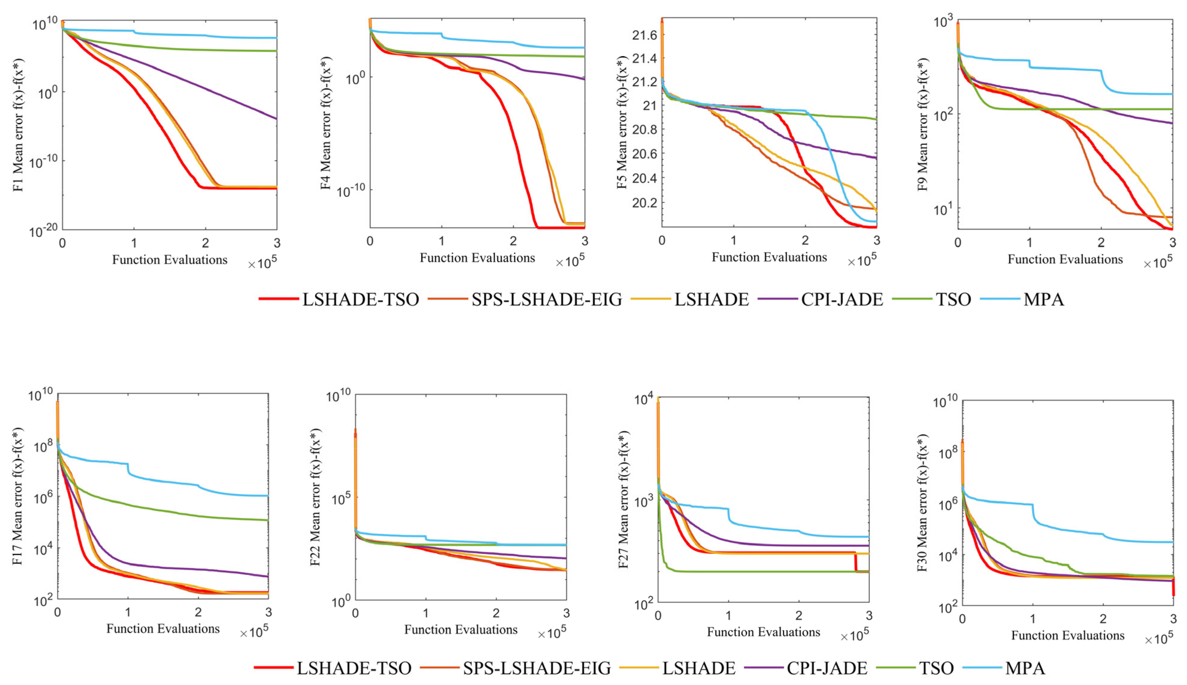
The CEC2014 test set contains 30 test functions, which can be divided into four types according to their different characteristics: F1–F3 for single-peaked functions, F4–F16 for multi-peaked functions, F17–F22 for mixed functions, and F23–F30 for combined functions; the definitions and optimal values of these functions can be found in the literature. The maximum number of evaluations (Maximum Function Evaluations, FEsmax) was set to D × 10,000, where D denotes the dimension of the problem. This section uses the CEC2014 30D function for testing, so FEsmax is equal to 300,000. The environment for simulation experiments was an AMD R7 4800 U (1.80 GHz) processor and 16 GB RAM, and the program was run on the MATLAB 2016b platform. Each algorithm was solved 51 times for each test function, and the mean and standard deviation were recorded.

In this paper, some of the four types of test functions are selected to demonstrate the convergence performance of the LSHADE-TSO algorithm. In Figure 5, f(x*) is the minimum value of the test function. It is clear shown in Figure 5 that the LSHADE-TSO algorithm converges faster and with greater accuracy in these test functions.

Table 2. Friedman test results.

Algorithm	LSHADE-TSO	SPS-LSHADE-EIG	LSHADE	CPI-JADE	TSO	MPA
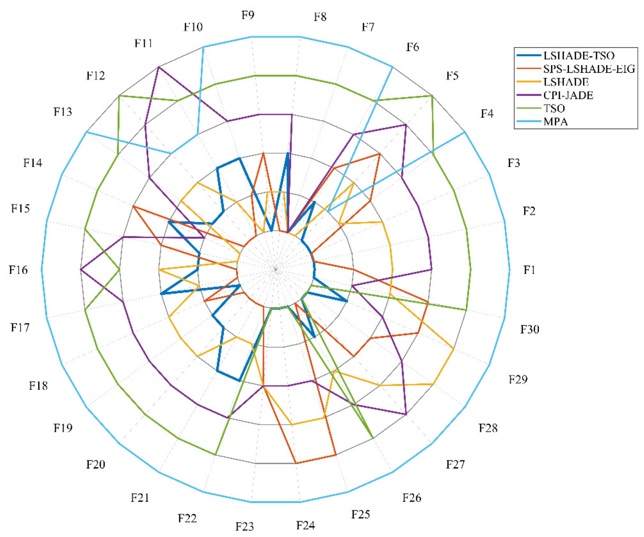
Rank	1.93	2.35	2.75	3.92	4.32	5.73

shows the ranking table of the algorithms obtained from Friedman’s test. There is no doubt that LSHADE-TSO is ranked first.

The algorithm ranking radar chart of the six algorithms is shown in Figure 6, and it can be seen that the LSHADE-TSO algorithm is ranked in the top two in most of the tested functions, with a few ranked third.

5. Simulation Experiments and Analysis

The aerodynamic parameters are the same for both red and blue, and the control variable limit range for both sides is $[{\alpha }_{\max },{\mu }_{\max },{\delta }_{\max }] = {[{34}^{\mathrm{o}}{,180}^{\mathrm{o}} ,1]}^{\mathrm{T}}$, $[{\alpha }_{\min },{\mu }_{\min },{\delta }_{\min }] = {[-{15}^{\mathrm{o}},-{180}^{\mathrm{o}} ,0.15]}^{\mathrm{T}}$. Both the UCAV and enemy initial control variables are $[{\alpha }_0,{\mu }_0,{\delta }_0] = {[0,0 ,0.5]}^{\mathrm{T}}$. The simulation time per step is set to 1 s (second). Both the enemy and the UCAV use the same vehicle platform, the initial distance between the two aircraft is 14.142 km, and the same type of infrared close-range air-to-air combat missile is mounted. ${\varphi }_{M\max }$ is set as 60°. The missile attack zone is solved using the method in the literature [44], and the air battle is set to end when the target remains for 5 s in the missile non-escapable zone. When the altitude is lower than 1000 m, it is determined that the air combat zone is exceeded, the simulation ends, and the winner is determined. This air combat simulation has been performed in many papers [24,36]; only the initial states and situation functions differ.

The initial state settings for the UCAV and enemy aircraft are shown in

Table 3. Initial state values of UCAV and enemy.

State	x	y	h	v	γ	Ψ (O °)	M (kg)
enemy	10,000	10,000	8000	250	0	225	14,680
UCAV	0	0	8000	250	0	45	14,680

.

5.1. LSHADE-TSO-MPC Maneuver Decision against Trial Maneuver Decision

The trial maneuver decision method is a more advanced maneuver decision method that has been proposed in recent years, which is characterized by rapid decision making, and its main method is to divide the control variable gradient so as to form a variety of optional control variable schemes, from which a maneuver trial is conducted to select a control volume scheme with the largest situation value. In this paper, the three control variables change range is divided into 11 gradients, thus forming 11 × 11 × 11 = 1331 medium maneuver schemes, whose gradient change values are set as follows:

$$\delta \in \left\{\begin{array}{c}{\delta }_{\min },{\delta }_{\min }/2,{\delta }_{\min }/4,{\delta }_{\min }/8,0\\ {\delta }_{\max },{\delta }_{\max }/2,{\delta }_{\max }/4,{\delta }_{\max }/8\end{array}\right\}$$

(36)

$$\alpha \in \left\{\begin{array}{c}{\alpha }_{\min },{\alpha }_{\min }/2,{\alpha }_{\min }/4,{\alpha }_{\min }/8,0\\ {\alpha }_{\max },{\alpha }_{\max }/2,{\alpha }_{\max }/4,{\alpha }_{\max }/8\end{array}\right\}$$

(37)

$$\mu \in \left\{\begin{array}{c}{\mu }_{\min },{\mu }_{\min }/2,{\mu }_{\min }/4,{\mu }_{\min }/8,0\\ {\mu }_{\max },{\mu }_{\max }/2,{\mu }_{\max }/4,{\mu }_{\max }/8\end{array}\right\}$$

(38)

The simulation results are shown below.

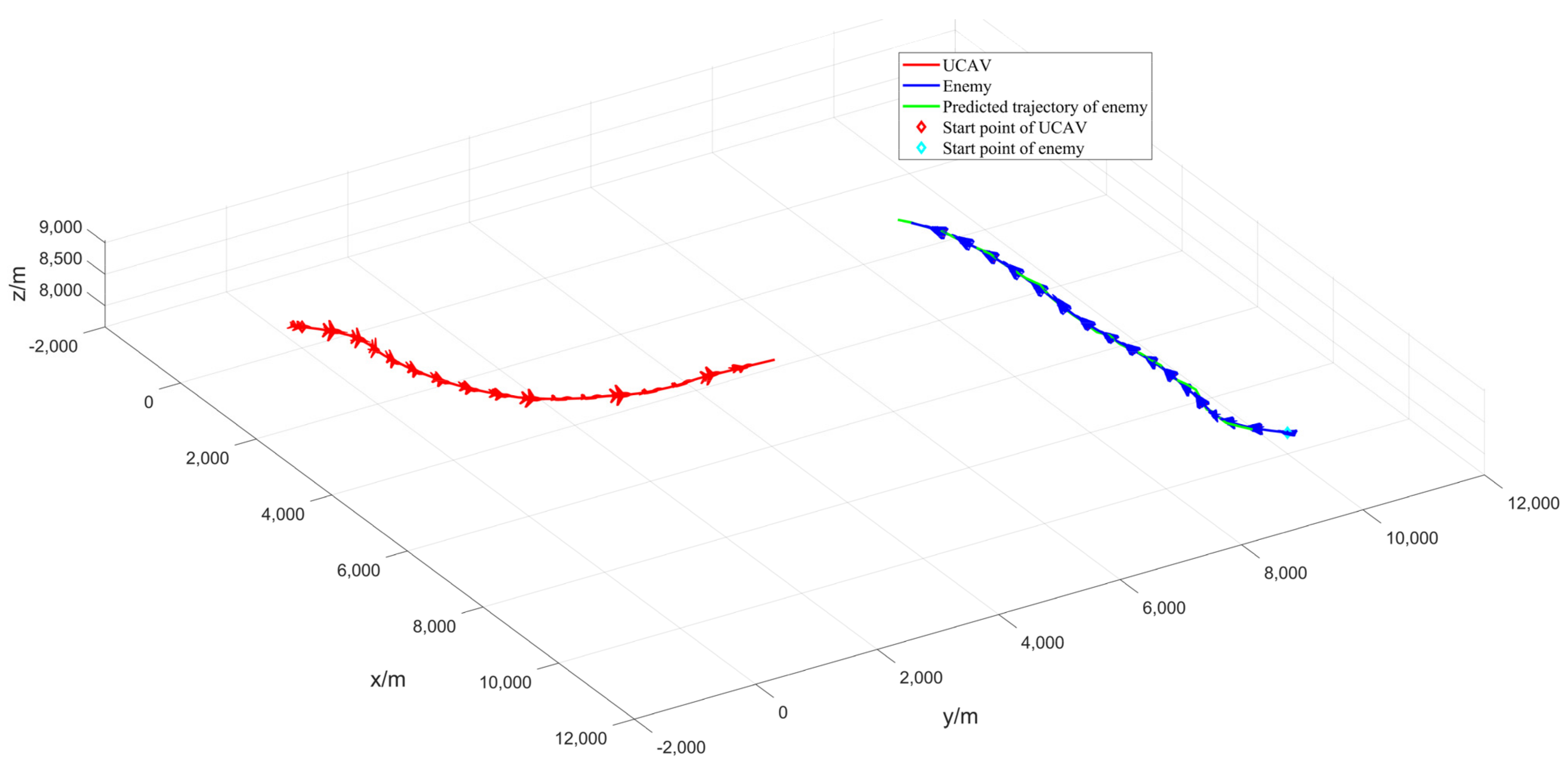
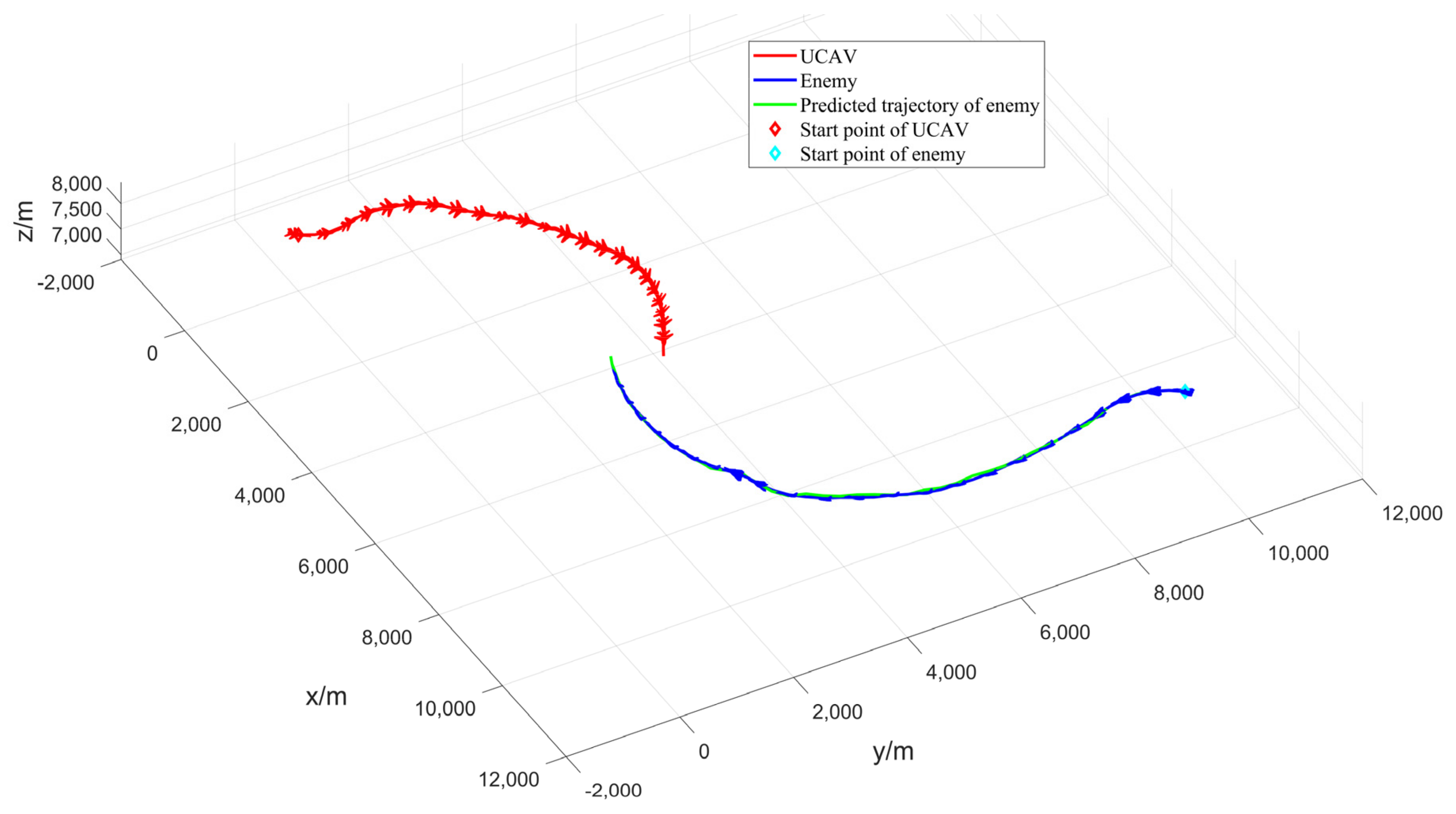
Figure 7 depicts the 3D trajectory of the UCAV and the enemy, as well as the predicted trajectory of the enemy. After 34 s, the enemy aircraft is in our aircraft’s missile inescapable zone for 5 s continuously within 29–34 s, and our aircraft finally wins the air battle. Figure 7 shows that both the enemy aircraft and our aircraft performed similar maneuvers, first a right turn followed by a left turn, because our aircraft and the enemy aircraft used the same attitude function. However, our aircraft uses the enemy aircraft’s online prediction information via the MPC framework to ultimately win the air combat.

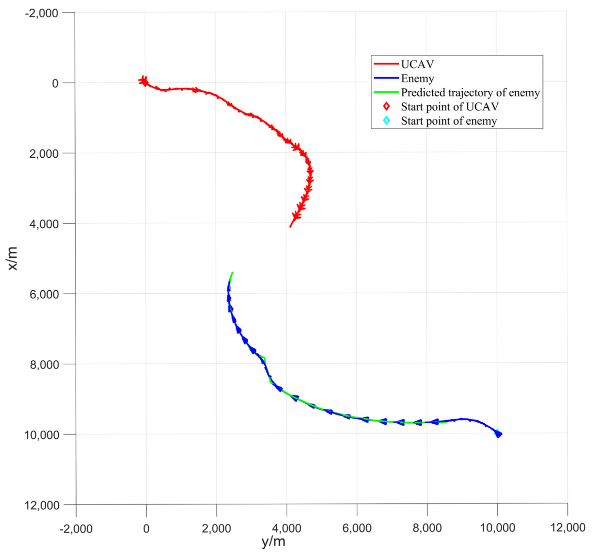
Figure 8 shows that the accuracy of predicting the trajectory of enemy aircraft decreases when they perform large maneuvers, such as some fluctuations in enemy aircraft predicted trajectory during right turns. In Figure 8, the predicted trajectory for the enemy aircraft is 3 s, and the length of one MPC control framework decision is also 3 s.

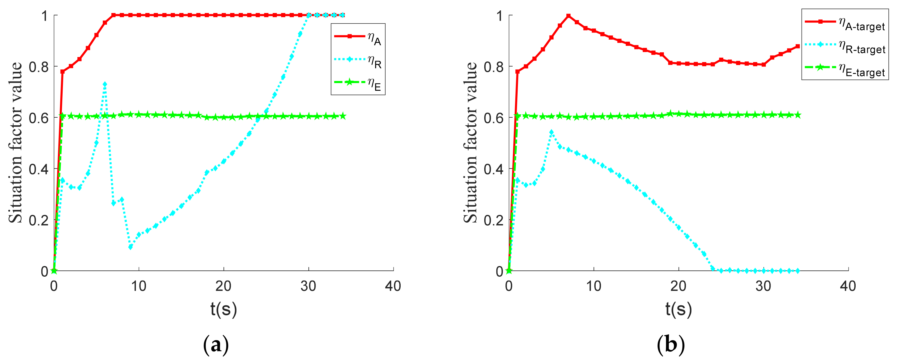
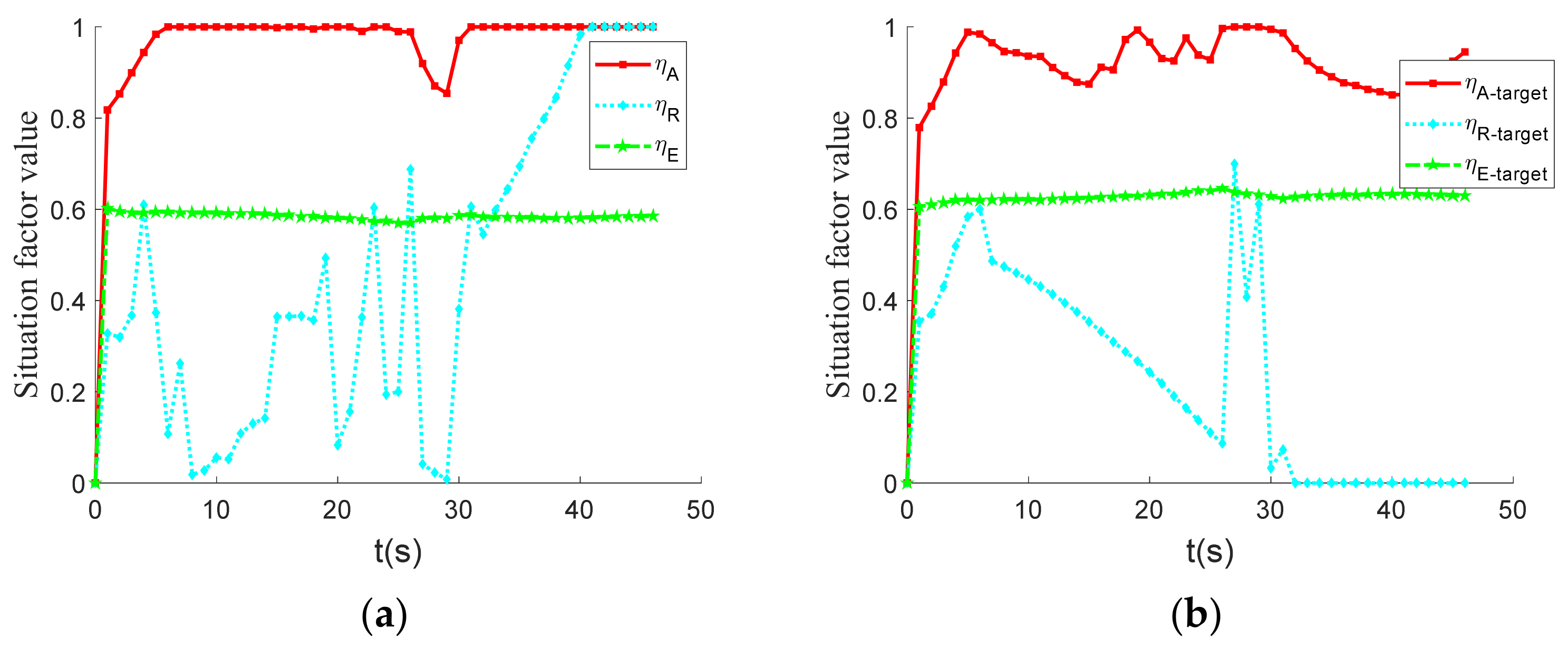
The graph above depicts the UCAV and enemy maneuver decision factor curves. Figure 9 shows that the angular situation factor value of our aircraft remains at 1 after rising in the initial stage, while the angular situation factor value of the enemy aircraft rises in the initial stage and gradually decreases. Because the enemy and our aircraft start at the same speed and altitude and perform similar maneuvers, their energy situation factor curves are similar. Our aircraft’s posture factor curve value continued to rise after a brief drop and eventually remained at 1, whereas the enemy aircraft’s distance posture factor value dropped to 0 in the final stage. The main reason for this is that the enemy is in the UCAV’s missile inescapable zone, and because the distance posture factor is coupled with the angular posture factor, the distance posture factor curves of the two aircraft differ significantly.

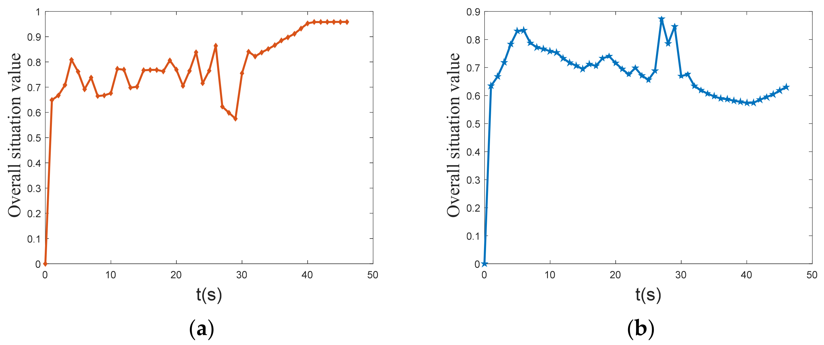
Figure 10 shows the overall situation value curves of UCAV and enemy. At the initial moment, the situation values of UCAV and enemy are the same, but after 34 s of maneuvering, the situation value of the UCAV reaches approximately 0.96, while the enemy’s situation value drops to approximately 0.56, and finally the UCAV wins the air battle. The overall situation value of the UCAV is greater than that of the enemy when the UCAV and the enemy use the same situation function, which shows that the maneuver decision method of the UCAV has a significant advantage over the enemy.

Figure 11 depicts the UCAV-enemy relative distance and missile inescapable distance curves. From 29–34 s, the enemy is in the UCAV’s missile inescapable zone for 5 s in a row, indicating that the UCAV has won the air battle. However, the enemy’s missile launchable distance is 0 because the enemy’s advance angle is greater than the missile’s maximum off-axis launch angle, preventing the missile from being launched and resulting in a 0 launchable distance.

Figure 12 shows that the advance angle of the UCAV is less than 60 degrees most of the time, indicating that the enemy is within the maximum off-axis firing angle of our missile most of the time, whereas the enemy’s advance angle is continuously less than 120 degrees from the eighths, indicating that the UCAV is continuously outside the maximum off-axis firing angle of the enemy’s missile.

Figure 13 shows the control variables curves of the UCAV and the enemy. The three lines from top to bottom represent the throttle, angle of approach and roll angle respectively. It can be seen that the control volume of the enemy aircraft is strictly on the gradient of the control volume range division, but our aircraft does not have this constraint in the control volume range. The control volume is a continuous variable, and the optimal control volume after discretizing it is likely to be in the gradient interval, which is why it is difficult for the trial maneuver decision method to beat the optimization algorithm decision method.

5.2. LSHADE-TSO-MPC Maneuver Decision against LSHADE-TSO Maneuver Decision

As shown in Figure 14, the three-dimensional trajectory of the UCAV and the enemy and the predicted trajectory of the enemy lasted for 46 s. Within 41–46 s, the enemy is in the inescapable missile zone of the UCAV for 5 s. Finally, the UCAV wins the air battle. As shown in Figure 14, both the UCAV and the enemy perform a left turn maneuver, but the UCAV performs a larger left turn and then a quick right turn. However, the UCAV makes a large left turn and then a quick right turn, whereas the enemy aircraft makes a small left turn followed by a near level flight and then a right turn, giving the UCAV the first opportunity to win the air battle.

Figure 15 shows the top view, from which we can see that the error between the predicted trajectory and the actual trajectory increases when the enemy performs a large overload maneuver with a prediction length of 3 s, which is reflected in Figure 15 as the distance between the green curve and the blue curve increases, showing a “burr” shape. In Figure 15, the predicted trajectory of the enemy aircraft is 3 s, and the length of one decision of the MPC framework is also 3 s.

Figure 16 depicts the UCAV and enemy maneuver decision factor curves. Figure 16 shows that the UCAV’s overall angular situation factor curve fluctuates from increasing to decreasing, then increasing again, and finally remaining at 1. The angular situation factor curve of the enemy aircraft undergoes a process from increasing and staying at 1 and then decreasing and then increasing again, but finally does not reach 1. The energy situation factor curves of the enemy and UCAV are similar and fluctuate in a very small range around 0.6. The distance situation factor of the UCAV factor fluctuates throughout the 0–30 s, but it increases rapidly after 32 s and eventually reaches 1. The distance situation factor value of the enemy aircraft decreases rapidly at 29 s and eventually drops to 0.

Figure 17 depicts the curve of UCAV and enemy overall situation value. The graph shows that the initial value of the overall situation of UCAV and enemy is similar. In the middle stage, the overall situation value of the enemy is clearly higher than that of the UCAV, but after 30 s, the overall situation value of UCAV increases rapidly, while the overall situation value of the enemy aircraft decreases. Finally, the overall situation value of the UCAV is stable at approximately 0.96, and the overall situation value of the enemy is stable at approximately 0.62. The UCAV’s situation value is significantly greater than the enemy’s, and it eventually wins the air combat.

Figure 18 depicts the UCAV’s and the enemy’s missile inescapable distance, as well as the two aircraft’s distance curve. In the 27–30 s time period, the enemy’s advance angle is less than the maximum missile off-axis launch angle, and the UCAV is within the enemy’s maximum missile off-axis launch angle. However, because the two aircraft are so far apart at this point, the UCAV does not enter the enemy’s missile-proof zone. The UCAV then maneuvers to successfully lasso the enemy into the missile inescapable zone and finally wins the air battle. From the missile launchable distance curve, the UCAV sacrificed some situational advantage when both sides were far away to gain a situational advantage when they were closer, which reflects the foresight of the LSHADE-TSO-MPC machine-dynamic decision method, which was able to consider the situational advantage at a longer distance, which has advantages over the optimization algorithm decision method.

Figure 19 shows the change curves of the advance angle between our aircraft and the enemy aircraft. Because the maximum off-axis launch angle of the missile is 60 degrees, the ATA of our aircraft fluctuates by approximately 60 degrees within 5–28 s, while the AA fluctuates by approximately 120 degrees. However, after 28 s, the ATA drops, while the AA fluctuates still around 120 degrees, and finally our aircraft achieves the air combat victory condition.

The three lines in Figure 20 from top to bottom represent the throttle, angle of approach and roll angle respectively. The curves of UCAV and enemy control variables shown in Figure 20 show that the change of angle of attack of the UCAV is more drastic than the enemy aircraft, and the throttle is not always in the maximum position, indicating that the UCAV can consider the relationship between speed and situation comprehensively, rather than just pursuing at maximum throttle and maximum speed.

5.3. Comparative Analysis of Different Algorithms Combined with MPC Framework

In the previous subsection we compared the LSHADE-TSO-MPC maneuver decision with the trial maneuver decision and LSHADE-TSO maneuver decision, and both achieved air combat victories, but we did not compare LSHADE-TSO-MPC with the rest of the optimization algorithms combined with the MPC framework. Therefore, this section confronts the maneuver decision methods of different optimization algorithms combined with the MPC framework with the LSHADE-TSO maneuver decision method. The simulation results are used to verify the performance of LSHADE-TSO-MPC compared to the rest of the optimization algorithms combined with the MPC framework.

The following methods are compared in this paper: LSHADE-MPC, TSO-MPC, and MPA-MPC for performance comparison, with a maximum of 50 iterations and a population size of 100, and the rest of each for comparison. The algorithm parameters are set as shown in

Table 4. Algorithm parameter setting table.

Algorithm Name	Parameter Setting
LSHADE	$N{P}_{init} = 100,N{P}_{\min } = 4,r^{arc} = 2.6,p = 0.11,H = 6,M_F = 0.5,M_{CR} = 0.5$
TSO	$a = 0.5,z = 0.05$
MPA	$FADs = 0.2,p = 0.5$

. The adversary employs the LSHADE-TSO maneuver decision, and the situation curves of both sides are obtained as shown in Figure 21. The time used for each maneuver decision method step are shown in Figure 22.

In PSO, C1 is the individual learning factor of the particle, C2 is the social learning factor of the particle, and $\omega$ is the inertia factor. In GA, Pc is the crossover probability and Pm is the variation probability.

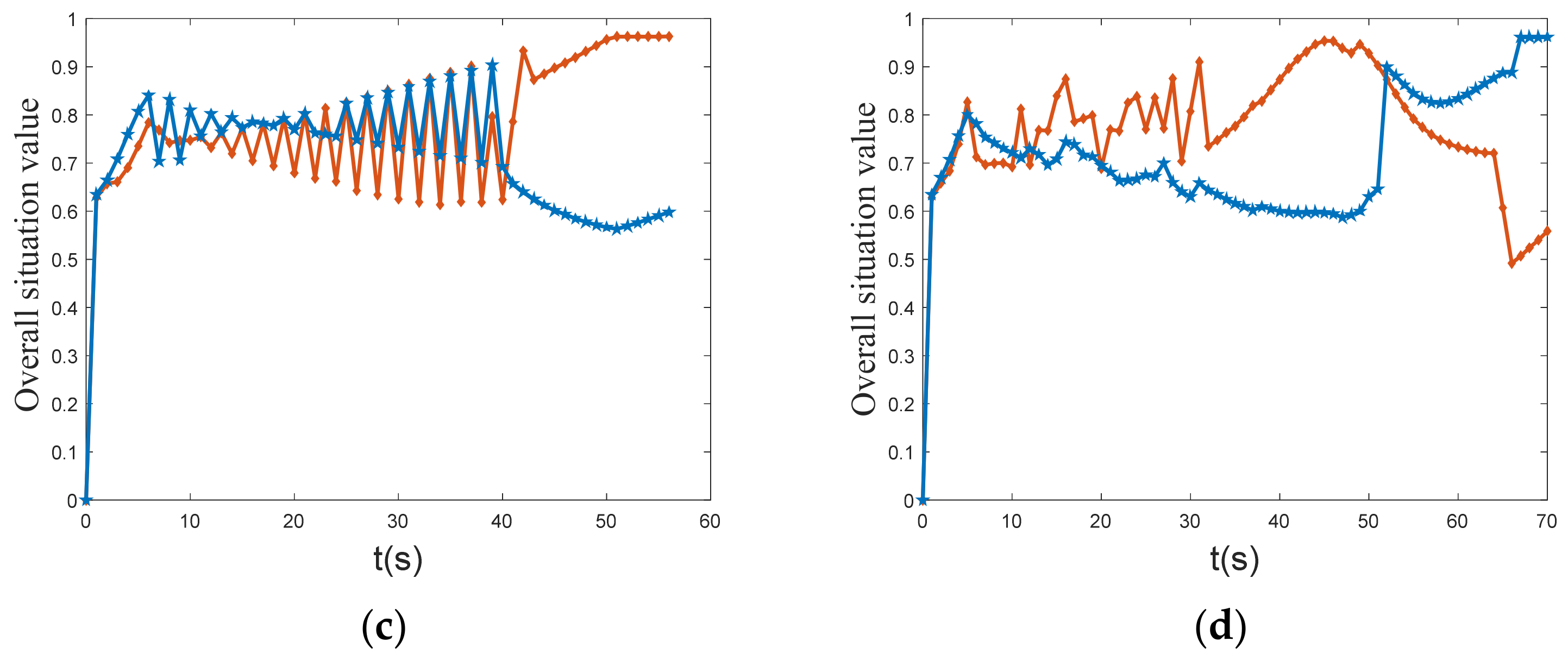
The overall situation value curves of both sides are obtained by combining LSHADE-MPC, TSO-MPC, and MPA-MPC with the LSHADE-TSO maneuvering decision, as shown in Figure 21. The results of the confrontation are presented in

Table 5. Four algorithms combined with the MPC framework against LSHADE-TSO.

Maneuvering Decision Making Methods	Air Battle Results	Air Combat Time
LSHADE-TSO-MPC	Win	46 s
LSHADE-MPC	Win	52 s
TSO-MPC	Win	56 s
MPA-MPC	Loss	70 s

. LSHADE-MPC achieved air combat victory in 52 s. GA-MPC achieved air combat victory in 56 s. At 70 s, the MPA-MPC was defeated by the enemy aircraft. LSHADE-TSO-MPC achieved air combat victory in 46 s. It is clear that the proposed LSHADE-TSO-MPC has some advantages over other optimization algorithms combined with the MPC framework, such as improved search and convergence capabilities.

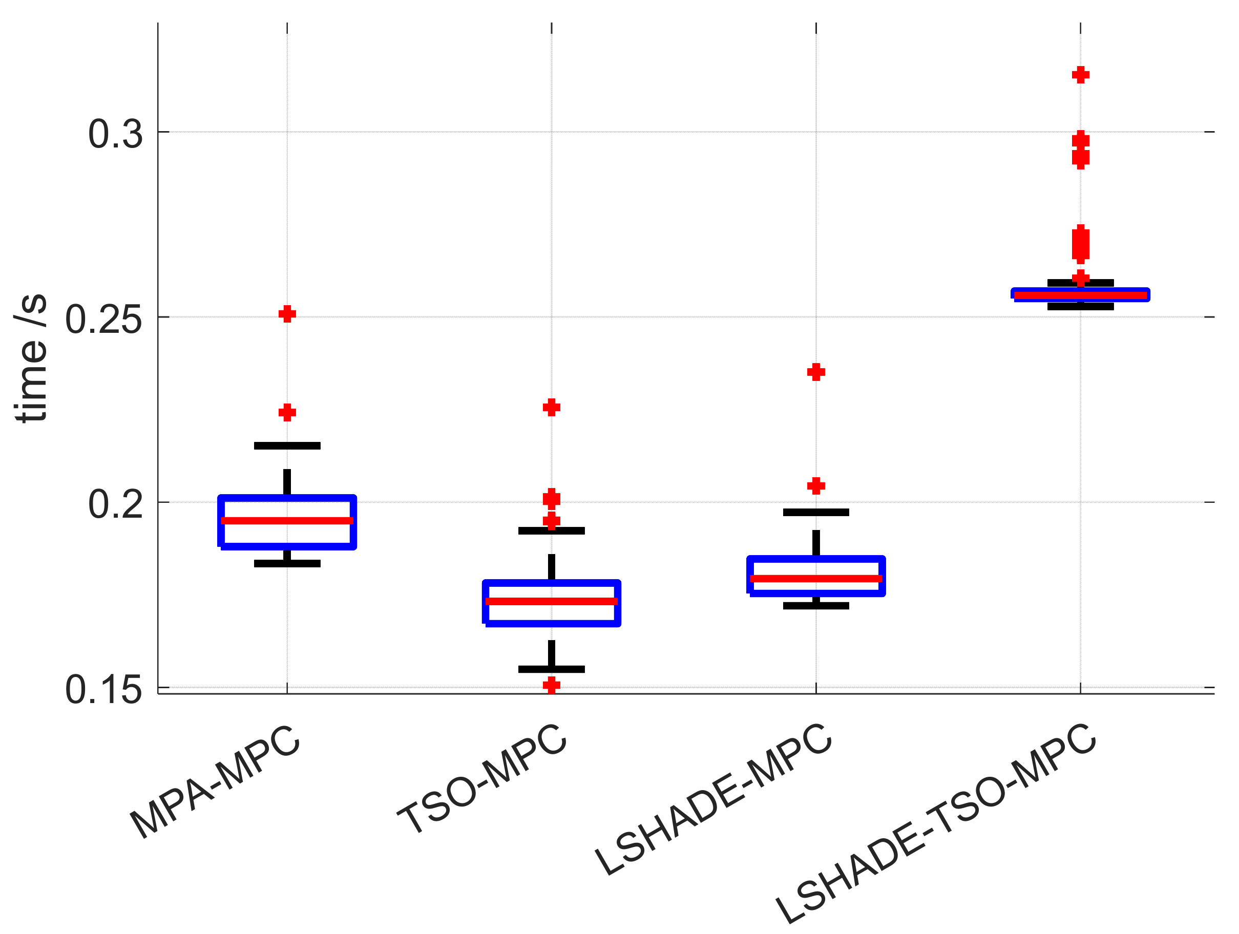
Figure 22 shows the comparison of the decision time used for the LSHADE-MPC, MPA-MPC, TSO-MPC, and LSHADE-TSO-MPC maneuver decision methods, where the average decision time of LSHADE-MPC is 0.1793 s, the average decision time of MPA-MPC is 0.1949 s, the average decision time of TSO-MPC is 0.1731 s, and the average decision time of LSHADE-TSO-MPC is 0.2557 s. From the results, the LSHADE-TSO-MPC has a longer decision time compared to the optimization algorithms in the literature [36], mainly due to the amount of control in deciding multiple steps in one decision, but it is acceptable compared to the 1 s decision cycle and can meet the real-time requirements.

6. Conclusions

In this paper, based on the traditional optimization algorithm for UCAV autonomous air combat maneuver decisions, an improved optimization algorithm is proposed for the solution of the maneuver decision problem, and the predicted trajectory of enemy aircraft is used for maneuver decisions in combination with a model predictive control framework. The method can incorporate future momentary posture into the objective function as well as expand the independent variable dimension, and more effectively exploit the advantages of intelligent optimization algorithms in high independent variable dimensional objective optimization. Using the same aircraft platform and weapon performance, a head-on air combat confrontation was conducted using the same posture function, and the results demonstrate that the use of a UCAV can effectively gain air combat advantage and achieve air combat victory under enemy trajectory prediction combined with model prediction control conditions. The LSHADE-TSO-MPC proposed in this paper has better decision-making capability in close air combat compared to other optimization algorithms combined with an MPC framework and can achieve air combat victory faster.

References

1. de Lima Filho, G.M.; Medeiros, F.L.L.; Passaro, A. Decision Support System for Unmanned Combat Air Vehicle in beyond Visual Range Air Combat Based on Artificial Neural Networks. J. Aerosp. Technol. Manag. 2021, 13, e3721. [Google Scholar] [CrossRef]
2. Pope, A.P.; Ide, J.S.; Micovic, D.; Diaz, H.; Rosenbluth, D.; Ritholtz, L.; Twedt, J.C.; Walker, T.T.; Alcedo, K.; Javorsek, D. Hierarchical Reinforcement Learning for Air-to-Air Combat. In Proceedings of the 2021 International Conference on Unmanned Aircraft Systems, ICUAS, Athens, Greece, 15–18 June 2021; pp. 275–284. [Google Scholar]
3. Luo, S.; Zhang, Z.; Wang, S.; Zhang, S.; Dai, J.; Bu, X.; An, J. Network for Hypersonic UCAV Swarms. Sci. China Inf. Sci. 2020, 63, 140311. [Google Scholar] [CrossRef] [Green Version]
4. Duan, H.; Shao, S.; Su, B.; Zhang, L. New Development Thoughts on the Bio-Inspired Intelligence Based Control for Unmanned Combat Aerial Vehicle. Sci. China Technol. Sci. 2010, 53, 2025–2031. [Google Scholar] [CrossRef]
5. Huang, Y. Modeling and Simulation Method of the Emergency Response Systems Based on OODA. Knowl.-Based Syst. 2015, 89, 527–540. [Google Scholar] [CrossRef]
6. Yuan, W.; Xiwen, Z.; Rong, Z.; Shangqin, T.; Huan, Z.; Wei, D. Research on UCAV Maneuvering Decision Method Based on Heuristic Reinforcement Learning. Comput. Intell. Neurosci. 2022, 2022, 1477078. [Google Scholar] [CrossRef]
7. Ma, W.; Li, H.; Wang, Z.; Huang, Z.; Wu, Z.; Chen, X. Close Air Combat Maneuver Decision Based on Deep Stochastic Game. Syst. Eng. Electron. 2021, 43, 443–451. [Google Scholar] [CrossRef]
8. Lee, B.Y.; Han, S.; Park, H.J.; Yoo, D.W.; Tahk, M.J. One-versus-One Air-to-Air Combat Maneuver Generation Based on Differential Game. In Proceedings of the 30th Congress of the International Council of the Aeronautical Sciences, ICAS 2016, Daejeon, Korea, 25–30 September 2016. [Google Scholar]
9. Virtanen, K.; Karelahti, J.; Raivio, T. Modeling Air Combat by a Moving Horizon Influence Diagram Game. J. Guid. Control. Dyn. 2006, 29, 1080–1091. [Google Scholar] [CrossRef] [Green Version]
10. Fu, L.; Xie, F.; Meng, G.; Wang, D. An UAV Air-Combat Decision Expert System Based on Receding Horizon Control. J. Beijing Univ. Aeronaut. Astronaut. 2015, 41, 1994–1999. [Google Scholar] [CrossRef]
11. Yang, Q.; Zhang, J.; Shi, G.; Hu, J.; Wu, Y. Maneuver Decision of UAV in Short-Range Air Combat Based on Deep Reinforcement Learning. IEEE Access 2020, 8, 363–378. [Google Scholar] [CrossRef]
12. Moon, J.; Papaioannou, S.; Laoudias, C.; Kolios, P.; Kim, S. Deep Reinforcement Learning Multi-UAV Trajectory Control for Target Tracking. IEEE Internet Things J. 2021, 8, 15441–15455. [Google Scholar] [CrossRef]
13. Ruan, W.; Duan, H.; Deng, Y. Autonomous Maneuver Decisions via Transfer Learning Pigeon-Inspired Optimization for UCAVs in Dogfight Engagements. IEEE CAA J. Autom. Sin. 2022, 9, 1639–1657. [Google Scholar] [CrossRef]
14. Yang, Z.; Zhou, D.; Piao, H.; Zhang, K.; Kong, W.; Pan, Q. Evasive Maneuver Strategy for UCAV in Beyond-Visual-Range Air Combat Based on Hierarchical Multi-Objective Evolutionary Algorithm. IEEE Access 2020, 8, 46605–46623. [Google Scholar] [CrossRef]
15. Li, W.-H.; Shi, J.-P.; Wu, Y.-Y.; Wang, Y.-P.; Lyu, Y.-X. A Multi-UCAV Cooperative Occupation Method Based on Weapon Engagement Zones for beyond-Visual-Range Air Combat. Def. Technol. 2022, 18, 1006–1022. [Google Scholar] [CrossRef]
16. Xu, G.; Wei, S.; Zhang, H. Application of Situation Function in Air Combat Differential Games. In Proceedings of the Chinese Control Conference CCC, Dalian, China, 26–28 July 2017; pp. 5865–5870. [Google Scholar]
17. Park, H.; Lee, B.Y.; Tahk, M.J.; Yoo, D.W. Differential Game Based Air Combat Maneuver Generation Using Scoring Function Matrix. Int. J. Aeronaut. Sp. Sci. 2016, 17, 204–213. [Google Scholar] [CrossRef] [Green Version]
18. Liu, Y.; Gao, X.; Shi, J.; Deng, L.; Chen, L.; Wu, J. Research on Decision–Making Method of Air Combat Embedded Training Based on Extended Influence Diagram. In Lecture Notes in Electrical Engineering; Springer: Berlin/Heidelberg, Germany, 2022; Volume 64, pp. 4529–4541. [Google Scholar]
19. Pan, Q.; Zhou, D.; Huang, J.; Lv, X.; Yang, Z.; Zhang, K.; Li, X. Maneuver Decision for Cooperative Close-Range Air Combat Based on State Predicted Influence Diagram. In Proceedings of the 2017 IEEE International Conference on Information and Automation, ICIA 2017, Macao, China, 18–20 July 2017; pp. 726–731. [Google Scholar]
20. Fu, Q.; Fan, C.L.; Song, Y.; Guo, X.K. Alpha C2-An Intelligent Air Defense Commander Independent of Human Decision-Making. IEEE Access 2020, 8, 87504–87516. [Google Scholar] [CrossRef]
21. Geng, W.X.; Kong, F.; Ma, D.Q. Study on Tactical Decision of UAV Medium-Range Air Combat. In Proceedings of the 26th Chinese Control and Decision Conference, CCDC 2014, Changsha, China, 31 May–2 June 2014; pp. 135–139. [Google Scholar]
22. Hu, D.; Yang, R.; Zuo, J.; Zhang, Z.; Wu, J.; Wang, Y. Application of Deep Reinforcement Learning in Maneuver Planning of Beyond-Visual-Range Air Combat. IEEE Access 2021, 9, 32282–32297. [Google Scholar] [CrossRef]
23. Piao, H.; Sun, Z.; Meng, G.; Chen, H.; Qu, B.; Lang, K.; Sun, Y.; Yang, S.; Peng, X. Beyond-Visual-Range Air Combat Tactics Auto-Generation by Reinforcement Learning. In Proceedings of the International Joint Conference on Neural Networks, Glasgow, UK, 19–24 July 2020. [Google Scholar]
24. Xuan, Y.; Zhou, K.; Wu, B.; Wang, X.; Liang, Y. A UCAV Maneuver Decision-Making Framework for One-on-One Air Combat. In Proceedings of the 2021 International Conference on Autonomous Unmanned Systems (ICAUS 2021), Changsha, China, 24–26 September2021; Volume 861, pp. 2568–2581. [Google Scholar] [CrossRef]
25. Du, H.; Cui, M.; Han, T.; Wei, Z.; Tang, C.; Tian, Y. Maneuvering Decision in Air Combat Based on Multi-Objective Optimization and Reinforcement Learning. J. Beijing Univ. Aeronaut. Astronaut. 2018, 44, 2247–2256. [Google Scholar] [CrossRef]
26. Peng, G.; Fang, Y.; Chen, S.; Peng, W.; Yang, D. A Hybrid Multi-Objective Discrete Particle Swarm Optimization Algorithm for Cooperative Air Combat DWTA. In Proceedings of the Communications in Computer and Information Science, Brunów, Poland, 23–25 November 2016; Volume 682, pp. 114–119. [Google Scholar]
27. Van Nguyen, L.; Phung, M.D.; Ha, Q.P. Iterative Learning Sliding Mode Control for Uav Trajectory Tracking. Electronics 2021, 10, 2474. [Google Scholar] [CrossRef]
28. Hermand, E.; Nguyen, T.W.; Hosseinzadeh, M.; Garone, E. Constrained Control of UAVs in Geofencing Applications. In Proceedings of the MED 2018—26th Mediterranean Conference on Control and Automation, Zadar, Croatia, 19–22 June 2018; pp. 217–222. [Google Scholar]
29. Altan, A.; Hacıoğlu, R. Model Predictive Control of Three-Axis Gimbal System Mounted on UAV for Real-Time Target Tracking under External Disturbances. Mech. Syst. Signal Process. 2020, 138, 106548. [Google Scholar] [CrossRef]
30. Wang, X.; Yang, R.; Zuo, J.; Xu, X.; Yue, L. Trajectory Prediction of Target Aircraft Based on HPSO-TPFENN Neural Network. Xibei Gongye Daxue Xuebao/J. Northwest. Polytech. Univ. 2019, 37, 612–620. [Google Scholar] [CrossRef]
31. Sighencea, B.I.; Stanciu, R.I.; Căleanu, C.D. A Review of Deep Learning-Based Methods for Pedestrian Trajectory Prediction. Sensors 2021, 21, 7543. [Google Scholar] [CrossRef] [PubMed]
32. Cao, Y.; Cao, J.; Zhou, Z.; Liu, Z. Aircraft Track Anomaly Detection Based on Mod-Bi-Lstm. Electronics 2021, 10, 1007. [Google Scholar] [CrossRef]
33. Schwenzer, M.; Ay, M.; Bergs, T.; Abel, D. Review on Model Predictive Control: An Engineering Perspective. Int. J. Adv. Manuf. Technol. 2021, 117, 1327–1349. [Google Scholar] [CrossRef]
34. Belloufi, A.; Assas, M.; Rezgui, I. Optimization of Turning Operations by Using a Hybrid Genetic Algorithm with Sequential Quadratic Programming. J. Appl. Res. Technol. 2013, 11, 88–94. [Google Scholar] [CrossRef]
35. Grauer, J.A.; Morelli, E.A. A Generic Nonlinear Aerodynamic Model for Aircraft. In Proceedings of the AIAA Atmospheric Flight Mechanics Conference, National Harbor, MD, USA, 13–17 January 2014. [Google Scholar]
36. Xie, L.; Ding, D.; Wei, Z.; Xi, Z.; Andi, T. Moving Time UCAV Maneuver Decision Based on the Dynamic Relational Weight Algorithm and Trajectory Prediction. Math. Probl. Eng. 2021, 2021, 6641567. [Google Scholar] [CrossRef]
37. Tanabe, R.; Fukunaga, A.S. Improving the Search Performance of SHADE Using Linear Population Size Reduction. In Proceedings of the 2014 IEEE Congress on Evolutionary Computation, CEC 2014, Beijing, China, 6–11 July 2014; pp. 1658–1665. [Google Scholar]
38. Zhang, J.; Sanderson, A.C. JADE: Adaptive Differential Evolution with Optional External Archive. IEEE Trans. Evol. Comput. 2009, 13, 945–958. [Google Scholar] [CrossRef]
39. Xie, L.; Han, T.; Zhou, H.; Zhang, Z.R.; Han, B.; Tang, A. Tuna Swarm Optimization: A Novel Swarm-Based Metaheuristic Algorithm for Global Optimization. Comput. Intell. Neurosci. 2021, 2021, 9210050. [Google Scholar] [CrossRef]
40. Zhou, Y.Z.; Yi, W.C.; Gao, L.; Li, X.Y. Adaptive Differential Evolution with Sorting Crossover Rate for Continuous Optimization Problems. IEEE Trans. Cybern. 2017, 47, 2742–2753. [Google Scholar] [CrossRef]
41. Stanovov, V.; Akhmedova, S.; Semenkin, E. LSHADE Algorithm with Rank-Based Selective Pressure Strategy for Solving CEC 2017 Benchmark Problems. In Proceedings of the 2018 IEEE Congress on Evolutionary Computation, CEC 2018, Rio de Janeiro, Brazil, 8–13 July 2018. [Google Scholar]
42. Guo, S.M.; Tsai, J.S.H.; Yang, C.C.; Hsu, P.H. A Self-Optimization Approach for L-SHADE Incorporated with Eigenvector-Based Crossover and Successful-Parent-Selecting Framework on CEC 2015 Benchmark Set. In Proceedings of the 2015 IEEE Congress on Evolutionary Computation, CEC 2015, Sendai, Japan, 25–28 May 2015; pp. 1003–1010. [Google Scholar]
43. Wang, Y.; Liu, Z.Z.; Li, J.; Li, H.X.; Yen, G.G. Utilizing Cumulative Population Distribution Information in Differential Evolution. Appl. Soft Comput. J. 2016, 48, 329–346. [Google Scholar] [CrossRef]
44. Li, A.; Meng, Y.; He, Z. Simulation Research on New Model of Air-to-Air Missile Attack Zone. In Proceedings of the 2020 IEEE 4th Information Technology, Networking, Electronic and Automation Control Conference, ITNEC 2020, Chongqing, China, 12–14 June 2020; pp. 1998–2002. [Google Scholar]
Figure 1. Schematic diagram of sliding window recursive prediction.
Electronics 11 03383 g001
Figure 2. Schematic diagram of Bi-LSTM network structure.
Electronics 11 03383 g002
Figure 3. Schematic diagram of the MPC framework process.
Electronics 11 03383 g003
Figure 4. Schematic diagram of UCAV pseudo-six degrees of freedom model.
Electronics 11 03383 g004
Figure 5. Convergence curves of the four algorithms. * represents the minimum value of the test function.
Electronics 11 03383 g005
Figure 6. Radar chart of algorithm ranking.
Electronics 11 03383 g006
Figure 7. Three-dimensional air combat trajectory and predicted trajectory map.
Electronics 11 03383 g007
Figure 8. Top view of air combat trajectory and predicted trajectory.
Electronics 11 03383 g008
Figure 9. Maneuver situation factor change curve. (a) UCAV; (b) enemy.
Electronics 11 03383 g009
Figure 10. Overall situation value change curve. (a) UCAV; (b) enemy.
Electronics 11 03383 g010
Figure 11. UCAV-enemy relative distance and missile inescapable distance curve. (a) UCAV; (b) enemy.
Electronics 11 03383 g011
Figure 12. ATA and AA change curves. (a) UCAV; (b) enemy.
Electronics 11 03383 g012
Figure 13. Decision process control variable curve. (a) UCAV; (b) enemy.
Electronics 11 03383 g013
Figure 14. Three-dimensional air combat trajectory and predicted trajectory map.
Electronics 11 03383 g014
Figure 15. Top view of air combat trajectory and predicted trajectory.
Electronics 11 03383 g015
Figure 16. Maneuver situation factor change curve. (a) UCAV; (b) enemy.
Electronics 11 03383 g016
Figure 17. Overall situation value change curve. (a) UCAV; (b) enemy.
Electronics 11 03383 g017
Figure 18. UCAV-enemy relative distance and missile inescapable distance curve. (a) UCAV; (b) enemy.
Electronics 11 03383 g018
Figure 19. ATA and AA change curves. (a) UCAV; (b) enemy.
Electronics 11 03383 g019
Figure 20. Decision process control variable curve. (a) UCAV; (b) enemy.
Electronics 11 03383 g020
Figure 21. Overall situation values of four algorithms combined with the MPC framework against LSHADE-TSO. (a) LSHADE-TSO-MPC; (b) LSHADE-MPC; (c) TSO-MPC; (d) MPA-MPC.
Electronics 11 03383 g021aElectronics 11 03383 g021b
Figure 22. Box plot of algorithm decision time.
Electronics 11 03383 g022