A Graph-Based Metadata Model for DevOps in Simulation-Driven Development and Generation of DCP Configurations

Abstract

With the goal of improving the quality of model-based development and to reduce testing effort, DevOps practices have gained more and more importance. However, most system engineers are not DevOps specialists, and there are a lot of manual steps involved when writing build pipelines and configurations of simulations. For this purpose, an abstract graph-based metadata model is proposed. This allows the autogeneration of scenario descriptions for simulations and code for the build server where the simulation environment is set up and executed. This is demonstrated by applying this process to the DCP standard. In this paper, we will discuss three simple use cases which are motivated by practical problems that arise in complex development environments and how the proposed solutions can be used to tackle them. Detailed descriptions and implementations of the use cases show how the proposed methods can be applied in practice and help solve the described problems. Furthermore, a Python implementation of a DCP master and a simple FMI-to-DCP wrapper are presented in this work.

1. Introduction

To tackle the growing complexity of software on electronic control units (ECUs) in cars or co-simulation of physical phenomena of different parts of the vehicle, the use of software development practices has risen. In particular, DevOps plays an important role. According to [1], DevOps is a set of practices intended to reduce the time between committing a change to a system and the change being placed into production while ensuring high quality. Although DevOps is well established in software development [2] to ensure quality and traceability [3,4], there remain challenges when simulations come into play. Simulations are often very complex and need a lot of expert knowledge from other fields such as mechanical or electrical engineering. Thus, there is a need to provide dedicated frameworks which need only little knowledge of DevOps tools like build servers to enable the application of modern and efficient development practices. Although graph-based methods are not new in DevOps [2,5], we focus on the specific challenges that arise in the development and deployment of co-simulations. During the SimDEV project, a cooperation between Volkswagen and Virtual Vehicle, different approaches were analyzed with regard to how to tackle the challenges arising in the context of simulations and how to tackle building and deployment of the necessary metadata descriptions of the involved building blocks. See [6,7] for an overview of the findings. It should also be noted that most involved functions and models are very simplistic. However, because the main focus of this works lies in the development process itself and not in the models that are developed, the use of more artificial examples is justified in this context.

When performing model-based engineering there may be several components available from previous or parallel projects. Thus, it would be convenient to integrate them in the current workflow and test the system in several variations (models, versions, or different parameters). Hence, it would be more efficient to allow automatic setup of existing artifacts and pipelines from an abstract description of the simulation provided in UML, SysML, or the SSP standard [8] and then generate the necessary simulation setup from that description, at least in a semi-automatic fashion. In [9], we presented this framework and a first use case, and in [10] we elaborate on the theoretical background of the used methods. For demonstration, the distributed co-simulation protocol (DCP) standard [11] was chosen because it allows abstract description of co-simulation configuration [12] for very different kinds of setups, such as the cyber-physical system and offline simulations. In contrast to the process model for the application of DCP in [13], we propose the description of simulation setups by graphs and the algorithmic processing of these graphs to allow automated configuration and deployment of simulation scenarios. To achieve this goal, an abstract graph data structure is introduced to build the link between system engineering tasks, DevOps, and co-simulation. Furthermore, it is shown that the data structure is suited for data transformations between general scenario descriptions and co-simulation scenarios, and we will discuss the implementation of the use cases.

It is also important to highlight that the performance of the involved software and algorithms is not the main focus in our considerations as they serve the purpose of improving workflows where steps in corrections and reiterations and the involved simulation runs can take hours, so it is still feasible if computations take a few more seconds or minutes in the background, as it should not impact overall performance when hours of work can be saved. One should also keep in mind that nowadays computation time is much cheaper then manpower.

This paper is structured as follows. Section 2 describes problems that arise in the practical development of simulations and cyber-physical systems. This is done on the basis of use cases that serve as illustrating examples in order to highlight structure of the described problems. This serves as motivation for the developed methods. Section 3 describes the methods used; this includes the graph-based methods for generating pipelines in an algorithmic manner as well as descriptions of the standards involved. In Section 4, the use cases and their implementation are described and how the proposed methods solve the described problems. Finally, Section 5 summarizes the results and Section 6 discusses the implications of this work.

2. Motivational Examples

In this section, three use cases which are motivated by real-life applications are presented.

2.1. Description of a Development Process: From Systems Engineering to Automatic Deployment

In this section, a typical process in development of simulation models and the roles involved are described. A use case originally motivated in [6,7] is presented. The challenges and potential benefits of applying dedicated DevOps methods are highlighted.

The following scenario is considered. A system engineer wants to test two related software components. Their common behavior defines a system, which is subject to usage in product development projects at a later point in time. They know that there are two prototypes from development available, but they want to rely on the nightly version to use the most up-to-date version. They want to experiment and incorporate small changes; hence the software components have to be built from scratch in a regular fashion. To use them, the system engineer has to

• get access to the code;
• build a pipeline (or script) to build the model; and
• set up a co-simulation scenario and run it.

Figure 1 shows a schematic of this process. The content of the red box highlights what the system engineer has to define. The code, shown in green boxes, is maintained by developers. The boxes in blue are related to process automation. Typically, a DevOps engineer is responsible for implementing these activities. A clear separation of tasks enables every member of the team to focus on their respective role in the process.

• The system engineer defines the system design including model boundaries, their scope, and, in particular, the flow of model signals between models. This can either be done from scratch or by working in part with previously established models.
• The model developer creates the models and their implementation according to the previously defined system design.
• The DevOps engineer provides build pipelines—or templates for build pipelines—to build the models and deploy the resulting instances of these models as artifacts.

Similarly, pipelines for running the simulation need to be provided. These pipelines should be as flexible as possible to be parameterized for different configurations and situations.

Although the tasks described in this section are manageable in general, they suffer from several well-known problems. First of all, the entire process is considered complex, and involves many different tasks as sources for faults and errors. Fixing problems is time consuming, and unnoticed errors can lead to disasters. In particular, setting up the infrastructure for builds is not always straightforward and needs proper configuration management. This includes setup of scripts, pipelines, specific software versions, etc. This may be an additional challenge for someone with little software engineering in their background. Even with the help of the developers and DevOps engineers, it may be cumbersome. Staff might not be available all the time. Reaction time might be limited, so several of the arising issues may not be fixed immediately. For these reasons it would be desirable to have a dedicated mechanism in place that can be at least partially automated.

2.2. Auto-Configuration of Co-Simulations

In the configuration of co-simulation scenarios, the graph structure of the underlying simulation is used to configure the co-simulation algorithm, i.e., how the participants should be coupled [14]. In [15], e.g., an optimization procedure is used to find the optimal trigger sequence in sequential co-simulation. In sequential co-simulation, the quality of the simulation result will depend on the order in which simulation participants perform calculations in each step. From the meta-information of how participants are connected to each other, which is condensed into the co-simulation graph, an optimal sequence can be derived and used in the simulation run. A participant that acts as a sink, e.g., can always be executed last whereas a source should be executed first. Most participants will be neither but have both inputs and outputs; their number and specific connections can give information on which trigger sequence may yield better results.

The application of graph-based methods [16] to analyze the signal flow of co-simulation scenarios and subsequently configure the master algorithm are instrumental to the field of co-simulation. This process fits very well in the presented framework of a co-simulation process graph, which the co-simulation graph is a part of. Thus, already established methods can be used to automatically generate co-simulation configurations and make use of the presented framework to automatically run various scenarios and evaluate the results.

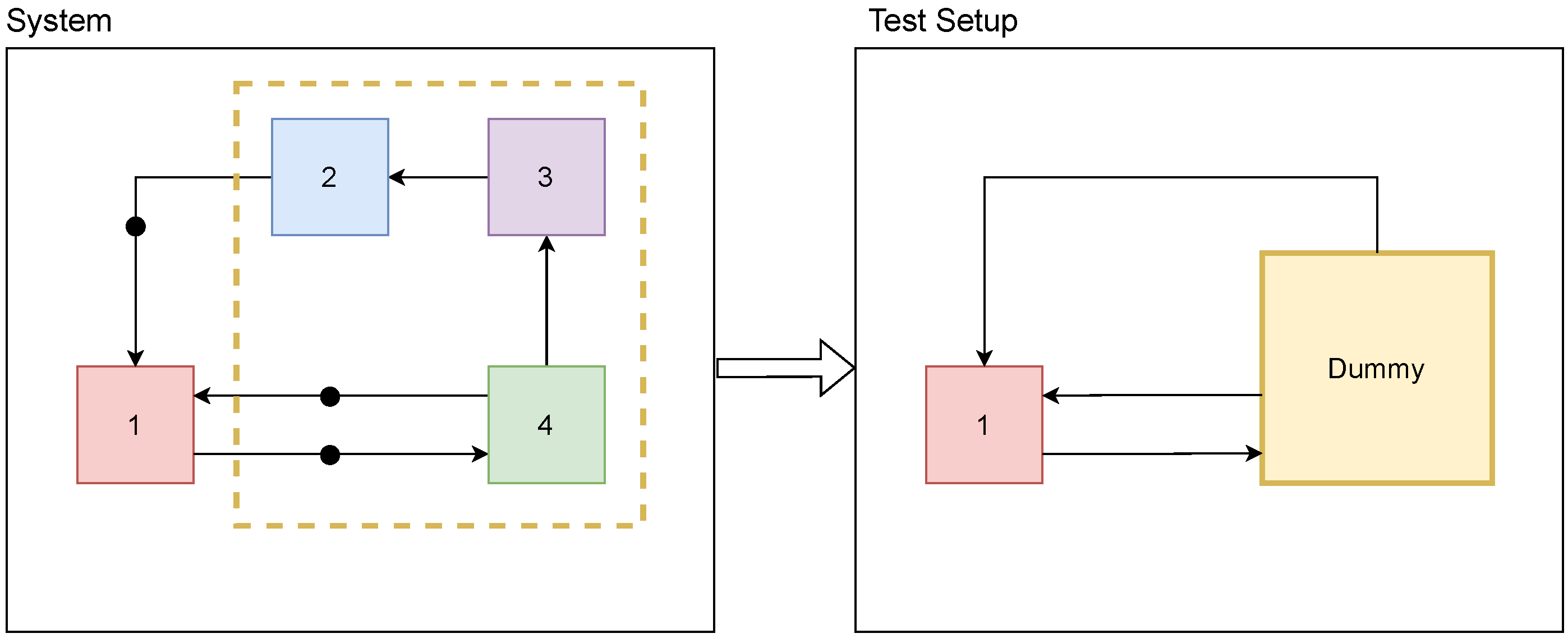
2.3. Automatic Test Generation from Already Executed Simulations

Another important application for a dedicated graph structure is the possibility of analyzing the failing of complex simulations, localize the error, and extract the faults to generate tests and enrich the build pipelines of components with suitable unit tests and subsystem integration tests. This is particularly a challenge in the context of cyber-physical systems where effects are often of physical nature and hard to predict. There are many methods by which to analyze errors with the help of graph structures. An example would be finding paths of error propagation [17]. However, many approaches rely on some previous knowledge (e.g., distribution of parameter etc.). Storing many test runs and their structure within a graph database allows one not only to improve the performance on the current run, but also to identify possible sources of error, extract subsystems, and generate new tests which can then be used for running tests in the future.

With the help of a dummy participant, tests can be created by using the logging information of a previous simulation run. Such a test dummy participant sends the recorded data from the other participants and can check the output the subsystems generated to emulate the run of the overall system in a more efficient way. This newly created subsystem is then turned into graph metadata and stored in the database. The main benefit of such an approach would be that the creation of a range of different test scenarios would get very time sensitive as they would have to be set up by hand in all different combinations. With the help of such a system, a semi-automatic approach can be used to easily enrich the test pipeline at each iteration when a new problem is identified, and it can easily be carried over to new versions of the participants under test. In this way, an increasingly robust test framework can be built in order to make test runs more efficient. Because the approach can also be applied to single participants, this opens the possibility for proper unit testing for models as well, as they often are hard to generate, as it is not always obvious how to perform basic functional tests for complex objects like simulations, contrary to simpler functions often appearing in conventional software development, where the behavior can be predicted more easily. For example, if in a complex simulation a fault is identified (for example a controller enters a wrong state), the inputs and outputs of the time when the wrong behavior happened can be extracted, and the wrong output could be checked against the expected output. This new dummy participant (which should run very fast) and this test setup could then be used by the developer of the component with the fault to debug it and add the gained unit test to the test pipeline. In this way, a check for regression is added to prevent the error to come back after future iterations.

3. The Co-Simulation Graph and the DCP Standard

In this section, we discuss the methods applied to the use cases described in the previous section and how we can address them with the help of appropriate data structures and co-simulation standards. The main contribution is the definition of the co-simulation process graph and dedicated methods to transform it. Although process graphs must be acyclic simulations, graphs will contain cycles due the involved feedback mechanisms. To remedy this, the sub-graph corresponding to the described simulation is contracted to a single node, thus giving a process graph that can be used to generate automation pipelines. This is done while maintaining the information within this contracted simulation node so that it can be expanded again at any time to the simulation graph to generate configuration data from its associated metadata. This section gives an overview of the used methods. A more detailed description of the data structure and analysis of the used algorithms can be found in [10].

3.1. Challenges and Contributions

The challenges described in the previous section can be overcome by developing and applying a dedicated process that allows the storage of configuration management data as metadata of the graph and process these graphs by appropriate algorithms. This approach is used in an effort to ensure traceability, reproducibility, and software quality by systematically automating the deployment of simulations. This work contributes by (1) introducing a method for setup of simulation-driven development processes that rely on graphs, (2) provision of an implementation consuming these graphs, automating the build process, and generate prototypical systems for simulation and testing, (3) using the leverage of graph databases for auto-configuration of co-simulations, and (4) providing suggestions regarding how the graph structure can be used to enrich the build process on the fly with component tests, which are generated from error reports.

3.2. Definition and Computational Framework for Co-Simulation Process Graphs

First, we start with a definition of the co-simulation process graph as a data structure. To model CI processes in DevOps, we introduce the concept of a pipeline. In [1] (p. 80f), a (deployment) pipeline consists of the steps that are taken between a developer committing code and the code actually being promoted into normal production, while ensuring high quality [18]. In more simple terms, a pipeline consists of process steps which must be executed in a certain order. These steps can be represented as a directed acyclic graph (DAG). We use the term DAG and pipeline synonymously in the context of this work.

Definition 1

(Pipeline). A pipeline is a directed acyclic graph, where each node represents a task inside the pipeline.

If a pipeline is given, a proper order can be computed efficiently, namely the topological order [19,20]. It should be noted that the major reason why directed acyclic graphs (DAGs) are used as a model is that they provide the possibility of generating the necessary execution steps offline. The benefits of an offline description are that static code can be generated which can be versioned and analyzed. This is important in the context of security and quality management in the DevOps process as it makes the automated processes more transparent and accessible for code analysis tools. However, when modeling pipelines for simulation processes, it is important to store the relations between different simulation participants inside scheduled simulations as well in order to provide efficient deployment orders and provide information on the used communication protocols and signals. This may introduce cycles inside the graph due to closed-loop simulations. This motivates the generalization of a DAG, namely the co-simulation process graph, a graph-based metadata model which allows the description of workflows and simulation scenarios in a unified manner and enables direct generation of the execution pipelines and auto-configuration of the simulations involved. This model is discussed in this section.

The co-simulation process graph was formally defined in [7] and is an extension of the classical process graph described in [21].

Definition 2

([7]). A co-simulation process graph is a directed graph with the following properties.

• The set of nodes consists of data nodes, transformation nodes, master nodes, signal nodes and communication (or gateway) nodes.
• To represent the instantiation of a process or the usage of a signal inside a simulation, copies of the nodes which represent these instances are made. Instances have to be directly connected to their originals.
• Instead of using the bi-partite structure to represent data transformations, only instances of processes can connect to data nodes to perform operations. In this way, the nodes which perform operations and their instantiation can be determined with a suitable algorithm, which determines a different partition of the graph with help of the defined structure, to provide the correct order of executions. This is necessary because it is allows that transformation nodes are neighboring, e.g., a Docker container which is built and then used for executing a program afterwards
• An information node can never be the successor or predecessor of another information node. A process must be placed in between. However, neighboring process nodes are allowed. This may happen if a program-performing transformation at a later stage is modified beforehand by another process (e.g., parameterization of tools).
• A simulation is a subgraph with the following properties: (a) It contains the instance of a master node. (b) The instance of the master node is connected to all instances of signal nodes that belong to the simulation. (c) All the other nodes inside the simulation (i.e., the simulation participants and communication gateways) neighbor a signal instance. (d) Each instance of a signal is only allowed to appear once inside a simulation.
• Cycles are only allowed inside a simulation subgraph.

An example is shown in Figure 2. A possible example is that the nodes $c_1$ and $c_2$ represent software sources (e.g., source code of a model), b represents a build tool like CMAKE and $b_1$ and $b_2$ represent two processes of this build tool which are started, which leads to the simulation units $P_1$ and $P_2$, while the node M represents a simulation master. After the build in stage 1) the simulation is executed, and the master is configured using the information contained in the node M and gets additional parameters from node I, whereas the node O represents the output of the simulation. The nodes $i_j$ and $o_j$ represent in- and outgoing signals like velocity or acceleration, whereas $g_j$ represents the communication protocols (e.g., a network protocol like IP) for $j=1,2$. This is depicted in Figure 3.

It can be shown that a co-simulation process graph can efficiently be transformed into a pipeline. This transformation consists of 2 steps:

1.

Scan and contract the simulations within the graph. This can be achieved by collecting the master nodes and collect all connected nodes, and their connected gateways. Then contract the simulation, i.e., all involved nodes in the simulation will be replaced by one node representing the simulation as a whole. This node is treated like a bridge, as the simulation can also be seen as a transformation from input data (e.g., configuration data) to output data (simulation results). See also [10] for a discussion of the efficient implementation of contractions within graph databases.

2.

Apply Algorithm 1 to transform the circle free co-simulation process graph into a pipeline.

These transformations are based on contractions which are of particular importance because they allow a simplification of the graph to make the representation more accessible for human users, because the data structure was designed to be computer friendly and can become quite complex.

The transformation nodes can also be filled with existing scripts and code snippets to improve the reusability of existing build scripts. This way the graph structure can be either directly used as a simple low code platform for programming pipelines or linked with existing technologies to make the combination of the continuous integration world with the realm of simulations easier. Because it is a universal data structure, it is not necessary to introduce new tooling but allows linking the existing tools into the framework.

Algorithm 1: Creating the vertices of a pipeline from an extended pipeline graph. Lists are denoted with square brackets.

See Figure 4 for the database view on the build graph for the adaptive cruise control (ACC) function as a further example. This graph contains all necessary steps for the build steps of the ACC function participant. Additionally, the database holds the signals which are associated with the participant which should be used in the scenario description for the DCP simulation. Several manufacturers have fixed catalogs of signals which are allowed to be used. Storing these in the database together with simulation participant helps developers to avoid using the wrong signals. Furthermore, this opens the possibility for algorithmic processing of the existing data.

In practice, teams can only focus on a local problem, but in a huge system more layers of complexity are added which are hard for humans to grasp. However, with a proper representation in a database these systems can be parsed and processed automatically. This enables complexity management of this problem, as it is difficult for humans to have a full overview of all aspects and more accessible for a computer to make a proper analysis of the huge amount of data. For example, consider optimization of the whole building process with limited resources, such as licenses, to avoid faulty local optimization of resource distribution.

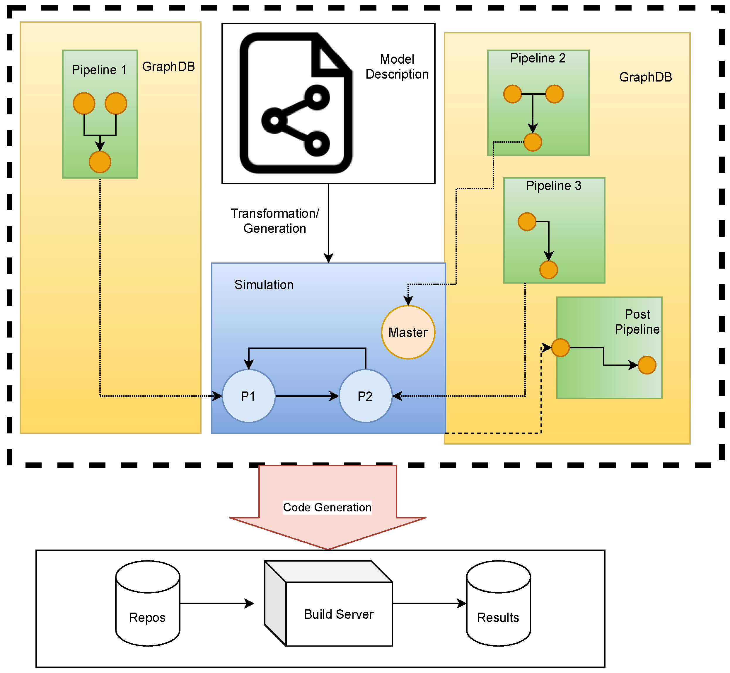
3.3. Graph Databases and the Metadata Model

In order to efficiently store graph-based structures, the obvious choice are graph databases as they allow us to map the co-simulation process graphs directly into the database without the need to transform the data in a form that is understood by relational databases. Furthermore, we can directly make use of the features of graph data bases to search for data with structural properties like neighboring edges. Graph databases can be defined in the following way.

Definition 3.

A graph database is a database whose data model conforms to some form of graph (or network or link) structure. The graph data model usually consists of nodes (or vertices) and (directed) edges (or arcs or links), where the nodes represent concepts (or objects) and the edges represent relationships (or connections) between these concepts (objects) [22].

There are several implementations of graph data bases like Neo4J, ArangoDB or OrientDB (see [23] for an overview and comparison of different graph data bases). For our purposes we use ArangoDB, as it allows us to directly store edges and nodes as text files (JSON). Additionally, the AQL query language is rather intuitive. ArangoDB simply stores the node data in JSON format. Edges are similarly stored as JSON, but they also contain the database identifier of the nodes which form the edge. This allows us to store the graph-based metadata, which is used in this work one-to-one in the DB.

The graph-based metadata model itself is defined in a flexible manner, as users can customize the transforming nodes to work with all kind of data and add data fields as needed. In the current examples only, (hyper-)links and text are used to avoid duplication of data. However, one could easily integrate transform nodes which can work with arbitrarily complex data and store them accordingly. The only restrictions are the unique identifiers of the node to be able to build and store the graph in a well-defined manner; everything else can be customized by the user. These identifiers are the ID (identifier), IID (instance identifier) and cls_name (type of node) fields. The (ID, IID) tuple as identifier has to be unique among all possible representations (e.g., when transforming among different databases which use their own identifiers). This allows for storing the data over different systems while keeping the graph well defined. The motivation why two main identifiers are used is that it allows one to use the same transforming bridge several times in the graph and therefore allows one to compute execution schedules offline. For example, there could be a node representing the Python interpreter with e.g., ID 1. However, the same interpreter can be now applied to several different scripts, e.g., script1.py, script2.py. Consequently, to represent the same program with two different parameters, one gets the three nodes with identifiers e.g., $(1,None)$, $(1,0)$, $(1,1)$, where None is reserved for the initial instance (namely the Python interpreter available) and $(1,0)$, $(1,1)$ represent the executions with script1.py and script2.py respectively. From this knowledge, an execution order can be computed offline based on how many resources are available. Note that the possibility of making the computations offline was a key motivator for this design, as pipelines for build services like Jenkins are only generated once and should not be changed during the run for reproducibility reasons, as it is possible to review and assess the generated code. As examples of how such nodes look, we included the JSON of some nodes of the first use case in the Appendix A (see Listing A1 for a normal data node, Listing A2 for a bridge node, Listing A3 for an instance of that bridge, and Listing A4 for an example of a signal node).

Another important aspect is the contraction of nodes for graphs and how to perform them efficiently in graph databases. This is important in order to simplify big systems or the remove cycles from graphs. A discussion and a detailed algorithm can be found in ([10], Chapter 3).

4. Implementation of the Use Cases

In this section, each of the use cases is described in detail highlighting how the proposed methods are used to overcome the problems described earlier.

4.1. Autogeneration of Co-Simulations from System Descriptions

This use case forms the basis for the subsequent use cases. In this use case, two models are connected in a simulation. The first is a model of an adaptive cruise control (ACC) system simply called ACC function that is to be tested. It controls the acceleration of a vehicle in order to maintain a desired speed by using incoming sensor data from the environment. In our case, the speed of the vehicle itself and the speed of and distance to the vehicle ahead if such a vehicle is detected are calculated. The second model encompasses the entire environment and serves as a counterpart to the ACC function. A system level description of the models, their signals, and how these signals are connected is shown in a UML diagram in Figure 5. Here, as an example, UML was used for the proof of concept, due to practical reasons as it was simple to realize as a showcase with open-source tools available. The UML metamodel that was used for demonstration is very primitive. The simulation master is described by a ProtocolStateMachine which holds properties (e.g., parameters for start time). The participants are classes which themselves have properties which hold parameters, and ports for the signals’ in- and outputs. The connectors are represented by InformationFlows, which hold the type of protocol encoded in the name. A simple but well-defined mapping into our graph model in the form of a simulation subgraph can be derived:

1.

A ProtocolStateMachine is mapped onto a master node. Its properties are added as data to the node.

2.

The class objects are represented as bridge nodes which again hold the property fields as information.

3.

The port objects are mapped onto signal nodes.

4.

The InformationFlow objects are then used to define connection nodes and the edges between the participants.

However, this approach is not limited to UML because other standards, such as SysML or SSP, could be used for the transformation as well because they are easily parseable. It should be highlighted again that this is a very simplistic model to showcase the viability of the approach. A more in-depth study of metamodels is needed to provide proper transfomrations for industrial use. Nevertheless, one can see that this should be extendable to other formats. This system description as it is designed by a systems engineer forms the basis of the use case and is used to generate the graph that describes the build and simulation framework. The structure of the process, which is described earlier in an abstract manner, is shown in Figure 6.

In this case, the model (green box) is maintained in a code repository by a developer and consists of C code as well as the model description in xml format. The build pipeline (blue box) is constructed by filling out templates of Jenkins pipelines with the following information. The location of and the access credentials to the code repository and used libraries and their location (here the FMU SDK), the model description (which we consider part of the code), and configuration of the model and its build environment. The resulting pipeline will compile the downloaded code into a shared library according to the provided configuration and package it together with the model description into an FMU. Then, the FMU is tested by using the FMU Checker to ensure formal compliance with the FMI standard and check if the shared object can be called by using the defined interface. Then, the resulting most recent version of the FMU is uploaded to an artifact repository. This forms a self-contained development process for each simulation unit in the scenario. This build process is repeated for all involved simulation participants.

To conclude the build stage of the process, these artifacts must be deployed in the simulation environment. Our implementation of the deployment uses docker containers. Each simulation participant, as well as the simulation master, is deployed in its own docker container, and the containers are started up and connected by using a docker network, this is schematically shown in Figure 7. Again, the configuration of these containers is generated automatically by using information contained in the co-simulation process graph, such as the number of participants, their connections and the network configuration.

The simulation stage of the process as depicted in Figure 2 gives information on the configuration of the scenario, in particular which signals are connected to which, which time step to use, how long to simulate, and so on. This is stored in the simulation graph and used to generate the configuration supplied to the master. The containers corresponding to simulation participants contain an FMI-to-DCP wrapper that allows the downloaded FMUs to be run as DCP participants once the container is started. This wrapper runs as a DCP slave that maps the state machine of DCP to that of the FMU, calling the appropriate FMI functions as triggered by the DCP master. This makes the functionality of the FMU available as a DCP participant. This wrapper was developed as a prototype by using the DCPLib  (https://github.com/modelica/DCPLib, accessed on 10 January 2022)—which is the open-source reference implementation of DCP. It provides an implementation of the protocol, including slave description generation, state machine transitions, and data exchange, and ensures compliance with the protocol. The actual calculation of the simulation participant is relayed to the FMU that the DCP is wrapped around. In our implementation, we use the FMILibrary (https://github.com/modelon-community/fmi-library, accessed on 10 January 2022) for that purpose. When a docker container containing a simulation participant is started, the DCP slave in the container is started and transitions to the DCP state Alive, awaiting instructions by the master.

Once all docker containers are started, the master registers the participants and rolls out the given configuration by using configuration protocol data units (PDUs) via the network using TCP/IP. This causes the DCP slaves to transition through their state machine and apply the supplied configuration acknowledging each received message. Once the simulation is started by the master simulation, time starts, and each DCP slave independently calculates the current time step sending their output to the other slave and receiving their inputs by using data PDUs. This is called the soft real- time (SRT) configuration of DCP, i.e., every simulation participant keeps their own time and performs the calculations in real time by best effort. Of course this is no problem in our minimal example, but in a real-world scenario care must be taken to ensure the performance of the models is adequate. Once a certain amount of wall clock time has passed, the master sends a stop PDU to each participants and notes their orderly termination. Then the results of the simulation are collected and uploaded to an artifact repository.

This use case is treated as a prototype that the other use cases are based upon Their configuration management and deployment follow the same principals, and the pipelines for building and deploying the simulation are automatically adapted to the changes in configuration.

4.2. Autoconfiguration of Execution Orders of Participants in Co-Simulations

As discussed in Section 2.2 the co-simulation graph is already used to analyze the system and generate configurations. Since the co-simulation process graph contains this graph in the simulation stage, these methods fit well in our proposed framework. In sequential non-iterative co-simulation (i.e., the execution of the models in each time step in a certain sequence without repeating steps), the order of execution is of importance for the quality of the result. In DCP, this sequential execution, which is important for the determinism of the system, is possible by using the non-real-time operating mode (NRT). In this mode, the simulation time is completely independent of the wall clock time and participants only calculate to the next time step when explicitly triggered to do so by the simulation master. Indeed, the sending of outputs is also triggered by the master to enable a more fine-grained configuration, such as which participants will receive which data during the sequence of execution. This represents the default mode in co-simulation in the FMI-specification [24]; however, due to the distributed nature of DCP, this is represented as separate state transitions. Note that in NRT this does not necessarily mean that the system is not running in real time, but rather that the time of each participant is dependent on triggers from the master. If all participants of an NRT system can perform their calculations in real time and the master can trigger these in real time, the system is running in real time.

In our use case, the sequence of execution of the simulation participants is a fixed configuration that can be changed as a parameter. Although this was sufficient to run the simulation several times with changed parameters and compare the results, in principle this trigger sequence can be derived from the simulation graph [15].

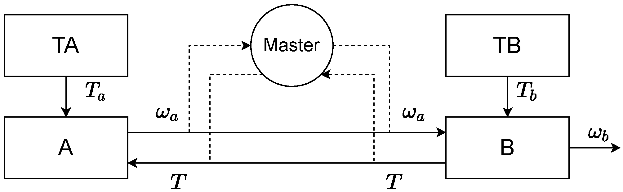
4.3. Autogeneration of Test Scenarios

As motivation, consider the following co-simulation, which represents a lumped propeller shaft [25] (see also Figure 8 for a schematic overview).

• The participant TA sends the time-dependent signal $T_a$ defined by the curve

  $$\begin{array}{c}\hfill T_a=\left\{\begin{array}{cc}0\hfill & \mathrm{if}0\le t<1,\hfill \\ a\hfill & \mathrm{else},\hfill \end{array}\right.\end{array}$$

  (1)

  with a = 10 Nm.
• Similar to TA, TB is defined by

  $$T_b=\left\{\begin{array}{cc}0\hfill & \mathrm{if}0\le t<2,\hfill \\ b\hfill & \mathrm{else},\hfill \end{array}\right.$$

  (2)

  with $b=-10 \mathrm{Nm}$.
• The system A is defined by the differential equation

  $${\dot{\omega }}_a=\frac{1}{J_A}(T_a-T)$$

  (3)

  with ${\omega }_A(t=0)=0$ and parameter $J_A=0.9 \mathrm{k}\mathrm{g}{\mathrm{m}}^2$.
• The system B is described by

  $${\dot{\phi }}_A={\omega }_A$$

  (4)

  $${\dot{\phi }}_B={\omega }_B$$

  (5)

  $${\dot{\omega }}_B=\frac{1}{J_B}\left(c({\phi }_A-{\phi }_B\right)+d\left({\omega }_A-{\omega }_B)-T_b\right)$$

  (6)

  with the initial conditions ${\phi }_A(t=0)=0$, ${\phi }_B(t=0)=0$, ${\omega }_B(t=0)=0$ and parameters $J_B=0.7 \mathrm{k}\mathrm{g}{\mathrm{m}}^2$, $c=1000 \mathrm{N}\mathrm{m}/\mathrm{rad}$ and $d=44.17 \mathrm{k}\mathrm{g}/\mathrm{s}$. The outgoing signal is determined by the relation

  $$T=J_B{\dot{\omega }}_B+T_a.$$

  (7)

A proper system initialization is needed in order to only couple the shafts when an equilibrium is reached to avoid undesired effects. In DCP, this can be achieved by use of the synchronization states indicating a finished synchronization by transitioning to the state Synchronized before starting the actual simulation. This can be achieved by implementing a coupling control in the master which can distinguish between an initial transient oscillation phase and the actual simulation run.

In certain simulation scenarios, it can be of vital importance to start the system from a consistent initial state. For this purpose, DCP provides a separate initialization phase called the super state Initialization comprised of several states. In contrast to the synchronization states, this is done before simulation time starts. Although this feature is optional, it can be used to run the simulation a number of non-real-time steps before the simulation time starts, even in real time operating mode. This can be used by the master to bring the system to a consistent initial state before the actual simulation is started. In order for the master to have control over the system, the data can be routed via the master in this initialization phase only and exchanged directly between the simulation participants during the actual simulation run. This is depicted in Figure 8 for our use case. The dotted connections of participant A and participant B with the master are only active during initialization. These connections may be informed by dependencies of the simulation models and may thus be generated based on the simulation graph. The master can decide when an equilibrium is reached based on the exchanged data and start the simulation run.

However, implementing such a master control can be difficult. Problems like these can arise, for example, in the context of test benches where the coupling of such a system has implications on the hardware. Thus, it is important to test such a master control properly, so a lot of tests are needed, and reproduction of faults and errors has to be fast. Although the example above is relatively simple, when faced with additional complexity creating tests becomes difficult and test runs may take a long time, as many participants may be needed to reproduce the issue and avoid regression over long-term development.

To tackle this issue, the following approach is proposed to ease up the creation of proper test cases in a timely manner. The left-hand side of Figure 9 shows a scenario with four participants (as in the example above). From a previous simulation, run-stored data is used to generate a test for participant 1, which can be seen on the right. The data of all inputs and outputs of participant 1 at the black dots is used to generate a test participant that simply repeats the recorded data. This is done by considering all participants, except for the one to be tested, to be in a subsystem and contracting this subsystem to a single new participant. This enables us to test participant 1 for repeatability and determinism, and this test can run cheaply again and again during continuous development of participant 1 without having to run the whole system again. In the same manner, tests for all other participants can be generated each time, putting all participants that are currently not to be tested in a subsystem, assuming all data from a previous simulation run has been recorded. We tested this setup only for one participant. We did this because the code to generate a test dummy as a counterpart to one participant was available. However, in principle the same can be done to test entire subsystems. The subsystem consisting of participants 1 and 2 could, e.g., be tested against the data provided by participants 3 and 4 and so on. In this manner, a large number of integration tests can be generated by using the same setup and ensuring reproducibility of the results during the development process. Because each test only repeats data, it is very fast to run and one could test a model without running a computationally expensive participant, such as an environment simulation, each time. If no previous simulation was run, the data could be replaced by data from requirements, specifying how a model should behave. In this manner, a complex simulation system can be constructed step by step, adding on components or subsystems one at a time.

5. Conclusions

We presented practical problems arising in the complex process of development and deployment of simulation models. Furthermore, a graph-based approach was presented for the setup and generation of build pipelines involving simulations. This demonstrates our proposed approach to develop consistent and overarching DevOps processes to reduce the overall effort and highlights how graph databases can be used to increase reusability. Additionally, a simple implementation to make FMUs available as DCP participants was presented, and our methods were studied on three use cases which are motivated by real-world applications in order to show the feasibility of the presented methods.

6. Discussion and Outlook

We propose graph-based methods to allow for the description and automated handling of parts of this process. This can be used to reduce cumbersome and error-prone manual configuration of simulation scenarios. Additionally, it enables the deployment of a far greater number of automatically generated simulation configurations, while reusing existing models. Traceability and reproduceability are ensured by such a process, in particular when graphs are stored in graph databases which are managed in a way that keeps pipelines operational. Using modern co-simulation standards and development tools ensures interoperability and future-proofs model development. The proposed methods aim to make modern development environments more efficient overall, allowing developers and researchers to focus on their respective core tasks.

There are several topics left open which we would like to address further. One aspect is the proper versioning of graph databases in order to ensure traceability of error and faults during tests. Another topic involves the generalization of the proposed graph data structure to more complex co-simulation graphs in order to combine existing co-simulation graph-based methodologies with our co-simulation process graph model.

Another important topic would be to extend the demonstrated methods to standardized system descriptions which are more advanced as the examples used in this work are mostly conceptional. Additionally, although standards such as SSP describe the system itself, we aim to also store configuration data of how the system is to be simulated, such as time step size, initialization, sequential or parallel execution, etc. in a consistent manner. An extension to map more sophisticated models in SSP and SysML 2.0. to the graph model is planned.

Furthermore, autoconfiguration of big co-simulations with the help of graph-based approaches will be an important issue to tackle to improve overall usability of the proposed methods.

References

- Bass, L.; Weber, I.; Zhu, L. DevOps: A Software Architect’s Perspective; Addison-Wesley Professional: New York, NY, USA, 2015. [Google Scholar]
- Leite, L.; Rocha, C.; Kon, F.; Milojicic, D.; Meirelles, P. A Survey of DevOps Concepts and Challenges. ACM Comput. Surv. 2020, 52, 1–35. [Google Scholar] [CrossRef]
- Palihawadana, S.; Wijeweera, C.H.; Sanjitha, M.G.T.N.; Liyanage, V.K.; Perera, I.; Meedeniya, D.A. Tool support for traceability management of software artefacts with DevOps practices. In Proceedings of the 2017 Moratuwa Engineering Research Conference (MERCon), Moratuwa, Sri Lanka, 29–31 May 2017; pp. 129–134. [Google Scholar] [CrossRef]
- Rubasinghe, I.; Meedeniya, D.; Perera, I. Traceability Management with Impact Analysis in DevOps based Software Development. In Proceedings of the 2018 International Conference on Advances in Computing, Communications and Informatics (ICACCI), Bangalore, India, 19–22 September 2018; pp. 1956–1962. [Google Scholar] [CrossRef]
- Rodrigues, M.R.; Magalhães, W.C.; Machado, M.; Tarazona-Santos, E. A graph-based approach for designing extensible pipelines. BMC Bioinform. 2012, 13, 163. [Google Scholar] [CrossRef] [PubMed]
- Balci, S.; Reiterer, S.; Benedikt, M.; Soppa, A.; Filler, T.; Szczerbicka, H. Kontinuierliche Integration von vernetzten Steuergerätefunktionen im automatisierten Modellierungs- und Build-Prozess bei Volkswagen. In Proceedings of the SIMVEC 2018, Baden-Baden, Germany, 20–21 November 2018. [Google Scholar]
- Reiterer, S.H.; Balci, S.; Fu, D.; Benedikt, M.; Soppa, A.; Szczerbicka, H. Continuous Integration for Vehicle Simulations. In Proceedings of the 2020 25th IEEE International Conference on Emerging Technologies and Factory Automation (ETFA), Vienna, Austria, 8–11 September 2020; Volume 1, pp. 1023–1026. [Google Scholar]
- Modelica Association Project SSP. SSP Specification Document; Version 1.0; Modelica Association: Linköping, Sweden, 2019. [Google Scholar]
- Reiterer, S.H.; Schiffer, C. A Graph-Based Meta-Data Model for DevOps in Simulation-Driven Development and Generation of DCP Configurations. In Proceedings of the 14th Modelica Conference 2021, Linköping, Sweden, 20–24 September 2021; pp. 411–417. [Google Scholar] [CrossRef]
- Reiterer, S.; Kalab, M. Modelling Deployment Pipelines for Co-Simulations with Graph-Based Metadata. Int. J. Simul. Process. Model. 2021, 16, 333–342. [Google Scholar] [CrossRef]
- Modelica Association Project DCP. DCP Specification Document; Version 1.0; Modelica Association: Linköping, Sweden, 2019. [Google Scholar]
- Krammer, M.; Benedikt, M. Configuration of slaves based on the distributed co-simulation protocol. In Proceedings of the 2018 IEEE 23rd International Conference on Emerging Technologies and Factory Automation (ETFA), Torino, Italy, 4–7 September 2018; Volume 1, pp. 195–202. [Google Scholar] [CrossRef]
- Krammer, M.; Schiffer, C.; Benedikt, M. ProMECoS: A Process Model for Efficient Standard-Driven Distributed Co-Simulation. Electronics 2021, 10, 633. [Google Scholar] [CrossRef]
- Gomes, C.; Thule, C.; Broman, D.; Larsen, P.G.; Vangheluwe, H. Co-simulation: State of the art. arXiv 2017, arXiv:1702.00686. [Google Scholar]
- Holzinger, F.R.; Benedikt, M.; Watzenig, D. Optimal Trigger Sequence for Non-iterative Co-simulation with Different Coupling Step Sizes. In Simulation and Modeling Methodologies, Technologies and Applications; Obaidat, M.S., Ören, T., Szczerbicka, H., Eds.; Springer International Publishing: Cham, Switzerland, 2021; pp. 83–103. [Google Scholar]
- Bastian, J.; Clauß, C.; Wolf, S.; Schneider, P. Master for Co-Simulation Using FMI. In Proceedings of the 8th International Modelica Conference, Dresden, Germany, 20–22 March 2011; pp. 115–120. [Google Scholar] [CrossRef]
- O’Halloran, B.M.; Papakonstantinou, N.; Giammarco, K.; Van Bossuyt, D.L. A graph theory approach to functional failure propagation in early complex cyber-physical systems (CCPSs). In INCOSE International Symposium; Wiley Online Library: Hoboken, NJ, USA, 2017; Volume 27, pp. 1734–1748. [Google Scholar]
- Roche, J. Adopting DevOps practices in quality assurance. Commun. ACM 2013, 56, 38–43. [Google Scholar] [CrossRef]
- Korte, B.; Vygen, J. Combinatorial Optimization; Springer: Berlin/Heidelberg, Germany; New York, NY, USA, 2012; Volume 2. [Google Scholar]
- Friedler, F.; Tarjan, K.; Huang, Y.; Fan, L. Combinatorial algorithms for process synthesis. Comput. Chem. Eng. 1992, 16, 313–320. [Google Scholar] [CrossRef]
- Tick, J. P-graph-based workflow modelling. Acta Polytech. Hung. 2007, 4, 75–88. [Google Scholar]
- Wood, P.T. Graph Database; Springer: Boston, MA, USA, 2009; pp. 1263–1266. [Google Scholar] [CrossRef]
- Fernandes, D.; Bernardino, J. Graph Databases Comparison: AllegroGraph, ArangoDB, InfiniteGraph, Neo4J, and OrientDB. In DATA; SciTePress: Porto, Portugal, 2018; pp. 373–380. [Google Scholar]
- FMI-Working-Group. Functional Mock-Up Interface for Model Exchange and Co-Simulation. 2020. Available online: https://github.com/modelica/fmi-standard/releases/download/v2.0.2/FMI-Specification-2.0.2.pdf (accessed on 12 April 2021).
- Benedikt, M.; Drenth, E. Relaxing stiff system integration by smoothing techniques for non-iterative co-simulation. In IUTAM Symposium on Solver-Coupling and Co-Simulation; Springer: Cham, Switzerland, 2019; pp. 1–25. [Google Scholar]
Publisher’s Note: MDPI stays neutral with regard to jurisdictional claims in published maps and institutional affiliations. |
© 2022 by the authors. Licensee MDPI, Basel, Switzerland. This article is an open access article distributed under the terms and conditions of the Creative Commons Attribution (CC BY) license (https://creativecommons.org/licenses/by/4.0/).
Share and Cite
Reiterer, S.H.; Schiffer, C.; Benedikt, M. A Graph-Based Metadata Model for DevOps in Simulation-Driven Development and Generation of DCP Configurations. Electronics 2022, 11, 3325. https://doi.org/10.3390/electronics11203325
Reiterer SH, Schiffer C, Benedikt M. A Graph-Based Metadata Model for DevOps in Simulation-Driven Development and Generation of DCP Configurations. Electronics. 2022; 11(20):3325. https://doi.org/10.3390/electronics11203325
Chicago/Turabian StyleReiterer, Stefan H., Clemens Schiffer, and Martin Benedikt. 2022. "A Graph-Based Metadata Model for DevOps in Simulation-Driven Development and Generation of DCP Configurations" Electronics 11, no. 20: 3325. https://doi.org/10.3390/electronics11203325
APA StyleReiterer, S. H., Schiffer, C., & Benedikt, M. (2022). A Graph-Based Metadata Model for DevOps in Simulation-Driven Development and Generation of DCP Configurations. Electronics, 11(20), 3325. https://doi.org/10.3390/electronics11203325