Abstract
The term NeuralODE describes the structural combination of an Artificial Neural Network (ANN) and a numerical solver for Ordinary Differential Equations (ODE), the former acts as the right-hand side of the ODE to be solved. This concept was further extended by a black-box model in the form of a Functional Mock-up Unit (FMU) to obtain a subclass of NeuralODEs, named NeuralFMUs. The resulting structure features the advantages of the first-principle and data-driven modeling approaches in one single simulation model: a higher prediction accuracy compared to conventional First-Principle Models (FPMs) and also a lower training effort compared to purely data-driven models. We present an intuitive workflow to set up and use NeuralFMUs, enabling the encapsulation and reuse of existing conventional models exported from common modeling tools. Moreover, we exemplify this concept by deploying a NeuralFMU for a consumption simulation based on a Vehicle Longitudinal Dynamics Model (VLDM), which is a typical use case in the automotive industry. Related challenges that are often neglected in scientific use cases, such as real measurements (e.g., noise), an unknown system state or high-frequency discontinuities, are handled in this contribution. To build a hybrid model with a higher prediction quality than the original FPM, we briefly highlight two open-source libraries: FMI.jl, which allows for the import of FMUs into the Julia programming language, as well as the library FMIFlux.jl, which enables the integration of FMUs into neural network topologies to obtain a NeuralFMU.
1. Introduction
Hybrid modeling describes, on the one hand, a field of research in Machine Learning (ML) that focuses on the fusion of First-Principle Models (FPMs), often in the form of symbolic differential equations and machine learning structures, such as Artificial Neural Network (ANNs). On the other hand, in the field of Ordinary Differential Equations (ODEs), hybrid models name the piecewise concatenation of continuous models over time to obtain a discontinuous model, of which the numerically simulated solutions may not be continuously differentiable over time. In this article, we present a workflow concerning both interpretations of hybrid modeling by integrating custom, discontinuous simulation models and ANNs into a discontinuous NeuralFMU. To illustrate, we use the example of learning a friction model for an industry-typical automotive consumption simulation based on a Vehicle Longitudinal Dynamics Model (VLDM).
In the following, the term hybrid model is used to identify a model based on the combination of an FPM and ML, whereas the concatenation of multiple continuous systems is referred to as a discontinuous model.
1.1. State of the Art: Hybrid Modeling
In the context of research applications, the structural integration of physical models into ML topologies, such as ANNs, is a topic that is receiving increasing attention. A simple approach to hybrid modeling is the integration of system knowledge into the Machine Learning (ML) process by evaluating equations of the physical model as part of the loss function, namely Physics-Informed Neural Networks (PINNs) [1]. In contrast, our method focuses not only on the evaluation of the physical equations in the cost function but also one step further on the structural integration of First-Principles Models (FPMs) directly into the Artificial Neural Network (ANN) or respectively the Ordinary Differential Equation (ODE) itself, offering more possibilities for manipulating and enhancing the ODE’s solution. Because the presented software allows for the differentiation of Functional Mock-up Units (FMUs), the building and training of PINNs is also possible with the presented libraries. Further, the field of hybrid modeling applies to stochastic system modeling as well, as shown in [2] using Bayesian Neural Stochastic Differential Equations (BNSDE), which feature the training of stochastic models on the basis of an optimization objective concerning Probably Approximately Correct (PAC) bayesian bounds. This reduces instabilities and enhances prediction accuracy. Moreover, Deep Auto-Regressive Networks (DARNs) can also be used to model physical systems. Similar to Recurrent Neural Networks (RNNs), the output of the last network inference is fed back into the neural network itself as input [3]. Different from RNNs, this feedback is not modeled as the neural network state, but as a simple feed-forward connection, and thus, a DARN can be trained as a conventional feed-forward network with all of the related simplifications and benefits. Finally, the combination of symbolic ODEs and object-oriented modeling languages, such as Modia, is a promising research field because of the benefits of acausal modeling [4]. References [5,6] provide a good overview of the expanding subject of hybrid modeling.
Retrieving a solution for a dynamic system includes the task of numerical integration. This task is difficult to perform for ANNs, e.g., a residual neural network, and requires a significant amount of training (considering especially higher-order and/or implicit integration methods). In contrast, ODE solvers are a long and well-studied chapter in numerical mathematics, and there are different optimized derivatives for almost any type of differential equation. Instead of numerically integrating with an ANN, an algorithmic numerical ODE solver is attached to the ANN in [7]. This leads to major improvements in computational performance and precision while offering a new range of possibilities, e.g., fitting the observed data at irregular time steps [8]. This integration of a numerical ODE solver into an ANN is known as NeuralODE, which is further introduced in Section 2.2. Despite the advantages listed, the transfer of the NeuralODE concept to real-world applications is not trivial, mainly for the following reasons:
- Real-world models from common modeling tools are in general not available as symbolic ODEs;
- NeuralODE training tends to converge in local minima;
- NeuralODE training often takes a considerable amount of calculation time.
Whereas the tendency to early converge to local minima and the long training times can be tackled by different techniques (Section 2.6 and Section 2.7), the major technical challenge hindering hybrid modeling in industrial applications remains: FPMs are modeled and simulated inside closed tools. ML features, the foundation allowing for hybrid modeling, are missing in such tools, and seamless interoperability with ML frameworks is not given. For example, for gradient-based training of the ANN parameters of hybrid models, the dependent loss function gradient must be determined through the ANN and FPM. This requires high-performance sensitivity algorithms, such as AD. ML frameworks, on the other hand, provide these abilities. To build high-performing hybrid models, an interface between these two application worlds is needed.
1.2. Preliminary Work: NeuralFMUs
In a preliminary publication [9], we faced this issue and expanded the concept of NeuralODEs by adding FPMs in the form of FMUs into this topology (Section 2.2). The resulting subclass of hybrid NeuralODEs, called NeuralFMUs, can be seen as the injection of system knowledge in the form of an FPM into the ANN model, which is equivalent to the right-hand side of the ODE.
Compared to the original FPM, the hybrid model introduces additional parameters (from the ANNs) that influence the dynamical system and can be used to enhance the model, e.g., in terms of prediction accuracy. In addition to enhancing prediction quality, the amount of necessary training data can also be significantly reduced because only the missing physical effects need to be learned. For example, the original FPMs were outperformed in terms of computational performance [10] and prediction accuracy [9] by being trained only on data gathered by a single, short part of the simulation trajectory. Further, the integration of an FPM can strongly enhance the extrapolation capabilities of the hybrid model compared to conventional purely data-driven models.
In this article, we want to follow up on these publications [9,10] by providing a workflow and results not only for a synthetic example but also for real-world application in the form of an energy consumption simulation based on a VLDM. The following challenges, which are common in industrial applications but are often neglected for scientific experiments, are overcome as part of this publication:
- Real measurement data: Training on real data raises challenges, such as noise and drifts. Whereas (small) uniformly distributed measurement noise may even improve the hybrid model’s quality by reducing overfitting, static sensor drifts must be identified and corrected. This can be completed with a state-correcting ANN, as highlighted later.
- Closed-loop controllers: Controlled systems may behave unexpectedly if the state dynamics are modified. Manipulating the dynamics of a controlled quantity forces the controller to compensate for these manipulations. On the other hand, this also offers possibilities. In the example of a velocity-controlled system introduced later, additional forces can be injected without changing the control value (velocity), as long the controller is robust enough to respond to the changes.
- Unknown system states: Dynamic systems in the industry often count many states. If a real demonstrator is used for data generation, usually not every state can be measured. This is a problem because the initial values of the system state are needed to solve the ODE inside of the FMU. If the data from computer simulations are sufficient, this is not an issue because, in general, simulation tools provide the capability to save every needed computation value.
- High-frequency discontinuities: As further introduced in Section 2.1, it is common to model ultra-fast continuous effects as discrete events. This way, instead of forcing the ODE solver to perform very small time steps, the solver is re-initialized after the event instance. This reset must be taken into account for the sensitivity determination. If the amount of time to reset the solver is smaller than the time to solve the original continuous system part, computation time can be saved. On the other hand, the excessive use of discontinuities, as in high-frequency sample-and-hold blocks, leads to long simulation times. Even if this can be avoided in many cases, it is a common modeling practice and needs to be taken into account.
This article is further structured into the following sections: a brief introduction to the standards used, the methods, the corresponding software libraries FMI.jl and FMIFlux.jl and the VLDM. These are followed by a presentation of the results of the example use case handling a NeuralFMU’s setup and training. Finally, the article closes with a conclusion and the future outlook.
2. Materials and Methods
In this section, a short overview of the standards, software and methods used is given. On this foundation, a workflow for setting up NeuralFMUs in real applications is given, and the methods for initialization and training are detailed. Finally, the VLDM, the FPM for the considered example use case, is introduced.
2.1. Functional Mock-Up Interface (FMI)
The FMI standard [11] allows for the distribution and exchange of models in a standardized format independent of the modeling tool. The interface standard counts three version releases. The most popular version is 2.0 [12], and the successor version 3.0 [13] was released in May 2022. Exported model archives that are compliant with the FMI’s specifications are called FMUs. FMUs can be imported into different simulation environments and organized into entire co-simulations, which again can be exported using a dedicated format called System Structure Parameterization (SSP) [14]. FMUs subdivide into three execution semantics: Model Exchange (ME), Co-Simulation (CS) and, new in FMI 3.0, Scheduled Execution (SE). The simulation mode highly depends on the FMU type and, further, the availability of standardized, but optionally implemented, FMI functions. The most relevant for the considered use case are MEs-FMUs because this type allows for manipulation and extension of the system dynamics before numerical integration.
To optimize simulation performance, fast physical effects, such as the change from stick- to slide-friction or the firing of an electrical diode, are often modeled in a discontinuous way. This means that the expressions of the right-hand side of the ODE model may change depending on the current system state and time, and this transition is discrete. Inside the FMI, this means ME-FMUs may contain state- or time-dependent discontinuities, which are triggering so-called events. The actual event’s time point, or the instant at which the equations and/or the state of the model is modified, is defined by a predefined time point itself (time events) or the zero-crossing of a scalar value (state-events), which is also called the event indicator. For a detailed overview of event definition and handling, see [13]. Basically, any ME-FMU with a continuous state , discrete state and time- and/or state-events can be seen as a discontinuous ODE, as shown in Figure 1. Continuous states may change in time, while discrete states can only change their value at event instances.
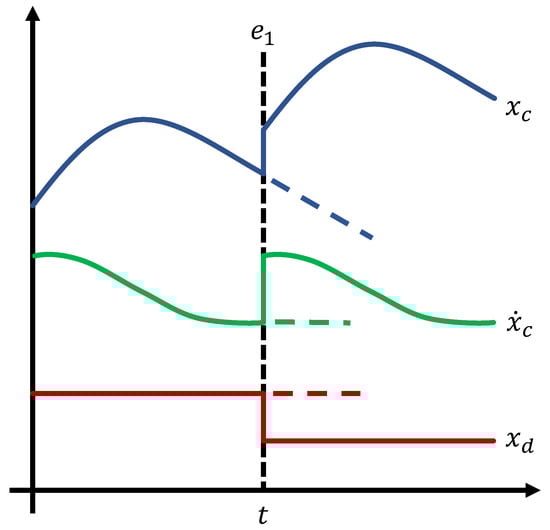
Figure 1.
Exemplified simulation of an ME-FMU with events (discontinuous ODE). The single (piecewise) continuous system state (blue) and state derivative may depend on a discrete system state (red), which is generally unknown for FMUs. Not handling events such as (black-dashed), leads to incorrect system values (blue-, green-, red-dashed) because the system state is not updated properly.
2.2. NeuralODEs & NeuralFMUs
NeuralODEs are defined by the structural combination of an ANN and a numerical ODE solver (see Figure 2). As a result, the ANN acts as the right-hand side of an ODE, whereas the solving of this ODE is performed by a conventional ODE solver. If the external requirements (tolerance or stiffness) change, the ODE solver can be easily replaced by another one. The scientific contribution, at this point, is not only the idea of this subdivision but also, more importantly, a concept to allow for training this topology on a target solution for the ODE. This requires propagation of the parameter sensitivities of the ANN through the ODE solver [7]. For training of NeuralODEs in the Julia programming language, the library DiffEqFlux.jl is available [15,16].
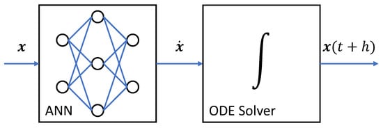
Figure 2.
Topology of a NeuralODE consisting of a feed-forward ANN and a numerical ODE solver. The current system state is passed to the ANN based on the following: the state derivative is calculated and integrated into the next system state by the ODE solver with the time step size h.
We expand the concept of NeuralODEs by one or more FPMs in the form of FMUs to obtain a class of hybrid models, named NeuralFMUs [9]. Using the example of an ME-NeuralFMU, the ME-FMU replaces the ANN of the NeuralODE because it calculates the system dynamics based on the current system state . To optimize the system state, an additional (state) ANN can be placed before the FMU, and, to manipulate the system dynamics, an additional (derivative) ANN can be placed after. This exemplified structure of a NeuralFMU is given in Figure 3.
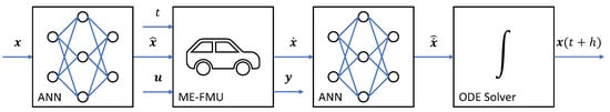
Figure 3.
Topology of an ME-NeuralFMU (example) consisting of two feed-forward ANNs, an ME-FMU and a numerical ODE solver. The current system state is passed to a (state) ANN. A manipulated system state is calculated and passed to the ME-FMU. There, the system state derivative is computed and manipulated by another (derivative) ANN into the changed system state derivative , which is finally integrated into the next system state by the ODE solver with the time step size h. Additionally, the FMU’s input , output or parameters (not shown) can be connected to the ANNs.
However, the concept of NeuralFMUs itself is very generic and does not restrict the positions or number of FMUs inside the ANNs or limit which signals are manipulated by the ANNs. The inference of a NeuralFMU can be reached by evaluating each of the considered blocks one after another. Whereas the evaluation of the derivative ANN (between FMU and solver) is straightforward because the system dynamics are passed as input to the ANN, inference of the state ANN needs additional attention. In case of an event inside the FMU, the FMU system state may be changed during event handling. This new state must be propagated backward through the state ANN to calculate a new system state at which the ODE solver is to reinitialize the numerical integration. Because ANNs are not invertible by default, the new state must be determined by solving an optimization problem. In the case of a state event, the required accuracy for the optimization solution is high because solving for a state that is slightly before the event instance triggers the event again. To prevent this, the optimization objective can be defined not only by hitting the FMU state but also by the change in the sign of the corresponding event indicator. This enhanced objective promotes finding a state that lies after the event instance in time. In the case of time events, high accuracy for the optimization result is desirable but not required.
For a more detailed overview of the concept of NeuralFMUs and the technical training process, see [9]. In the following, only ME-NeuralFMUs are considered and identified by the shortened term NeuralFMU.
2.3. Software
Combining physical and data-driven model parts and training the resulting hybrid structure is currently not possible inside a single industry tool. Therefore, a transfer of the FPMs between the conventional modeling and a more suitable ML environment is needed. After exporting from the modeling and importing into the ML environment, the first principle is extended to the hybrid model and trained on data. After successful training, it is necessary to re-import the hybrid model back into the original (or another) modeling environment for further modeling or to set up larger system co-simulations. For the considered importing and exporting between environments, a model exchange format with industrial relevance is needed. The FMI is an open standard that shows great popularity in large areas of the industry and research, and, therefore, it was picked as the model exchange format. In addition to modeling and simulation software, the FMI is already implemented in many common tools, but a software interface integrating the FMI into Julia, which is used as the ML environment here, is still needed (Section 2.3.2).
2.3.1. Julia Programming Language
In this section, the authors justify their choice of the Julia programming language (short: Julia) as the ML environment in which to deploy NeuralFMUs. Julia is a dynamic typing language that aims to provide fast numerical computations in a platform-independent, high-level programming language [17]. The language and interpreter were originally invented in 2009 and were released in 2012 by the Massachusetts Institute of Technology, At present, many other universities and research facilities provide language expansions and libraries.
In addition to the many great libraries in the field of scientific machine learning, there are multiple libraries for AD, e.g., ForwardDiff.jl [18,19] and Zygote.jl [20,21]. Many libraries provide low-level interfaces that require a good understanding of the methodology but allow high-performance implementations. Finally, even object-oriented modeling, syntactically similar to Modelica®, is possible with the library Modia.jl [22,23].
2.3.2. FMI in Julia: FMI.jl
In [9], we introduced the software library FMI.jl [24], which originally allowed for the import, parameterization and simulation of FMI2-FMUs in the Julia programming language. Since its first release, additional features have been added, such as a prototypical export for FMUs and support for FMI3. A feature worth mentioning is that FMI.jl allows for the simulation of FMUs with the same user front end independent of the FMI version. Loading and simulating the FMU, independent of the FMI version and simulation interface, can be achieved only by a few lines of code, as in Listing 1.
| Listing 1. Simulating FMUs with FMI.jl. |
 |
For experienced users, the low-level commands from the FMI specifications [12,13] are also wrapped into Julia commands. The library supports CS- and ME-FMUs, including proper event handling for discontinuous ME-FMUs. The entire FMI command set, including optional functions such as fmi2GetDirectionalDerivative and fmi2GetFMUState, is implemented. For more information about FMI.jl, see [9] or the library repository.
2.3.3. NeuralFMUs in Julia: FMIFlux.jl
Based on FMI.jl, the library FMIFlux.jl [9,25] provides an interface between an imported FMU and the Julia ML ecosystem. The setup and training of ANNs in Julia are predominantly made with the library Flux.jl [26], whereas NeuralODEs are modeled with DiffEqFlux.jl.
As in many other ML libraries, ANNs in Flux.jl are expressed as a sequence of layer operations. FMIFlux.jl provides the interface needed to use imported FMUs just as any other ANN layer. This includes providing the sensitivities between the FMU inputs and outputs for the Julia AD frameworks. As a result, similar to conventional deep ANNs, NeuralFMUs can also be expressed as a series of layers, including at least one FMU layer. A code example about the setup and training of a NeuralFMU (as in Figure 3) is given in Listing 2.
| Listing 2. Setup and training of an ME-NeuralFMU as in Figure 3 with n states in Julia. |
 |
FMIFlux.jl allows for a wide range of possible NeuralFMU topologies and does not restrict:
- The FMU variables used as the layer inputs and outputs. Any variable that is accessible via fmi2SetReal or fmi2SetContinuousStates is a potential layer input, and any variable that can be obtained by fmi2GetReal or fmi2GetDerivatives can serve as a layer output;
- The number and positions of the FMUs inside the ANN topology as long as the signal traceability via AD is given.
Dependent on the embedded FMU type, ME, CS or SE, different setups for NeuralFMUs should be considered. In this article, only ME-NeuralFMUs are highlighted. For more detailed information about FMIFlux.jl or other NeuralFMU topologies, see [9].
2.4. Workflow
On the foundation of Julia, FMI, FMI.jl and FMIFlux.jl, we suggest a workflow as in Figure 4 for designing custom NeuralFMUs. The presented development process of a NeuralODE/FMU covers the following steps; Steps 5–7 are optional and relevant only if the hybrid model will be re-imported into another simulation environment:
- The FPM is designed by a domain expert inside a familiar modeling tool that supports FMIs (export and import).
- After modeling, the FPM is exported as the FMU.
- The FPM–FMU is imported into Julia using FMI.jl.
- The FPM is extended to a hybrid model and trained on data, for example, of a real system or a high-resolution and high-fidelity simulation, using FMIFlux.jl. Simulation of the trained hybrid model and export of the simulation data is possible directly in Julia.
- The following steps are optional. The trained hybrid model may be exported as an FMU using FMI.jl.
- The hybrid model FMU may be imported into the original modeling environment or another simulation tool with FMI support.
- The improved hybrid model FMU may further be used as a stand-alone or as part of larger co-simulations, such as for example the distributed simulation framework in [27].

Figure 4.
Workflow of the presented hybrid modeling application using a modeling tool that supports FMI (export and import) and FMI.jl together with FMIFlux.jl.

2.5. Data Pre- and Post-Processing
In many ML applications, pre- and post-processing are not only instrumental but necessary. For training conventional ANNs, the pre-processing of training data can often be performed one single time before batching and the actual training. For NeuralFMUs, the FMUs may generate outputs within a range that is excessively saturated by the activation functions inside the ANN. Further, the FMUs may expect inputs within a range not generatable by the ANN because of the limited output of the activation functions. Therefore, all signals must be processed at the interfaces between the FMUs and ANNs.
If no expert knowledge of the data range of the FMU inputs and outputs is available, a good starting point can be to scale and shift data into a standard normal distribution. Because the FMU output and input may shrink or grow during training due to new state exploration by the changed dynamics, scaling and shifting parameters should be parts of the optimization parameters during training. See Section 3.2 for a visual example of a topology that uses data pre- and post-processing around an ANN.
2.6. Initialization (Pre-Training)
Obtaining a trainable (solvable) NeuralFMU is not trivial. The use of larger or complex FMUs together with randomly initialized ANNs often leads to an unstable and/or stiff ODE system. Further, model assumptions in the form of code assertions may be included in FMUs; these assertions are not guaranteed to be satisfied by the modified model. Whereas starting the training process with an unnecessarily stiff NeuralFMU (stiffer than in the final solution) leads to long training times, an unstable system might not be trainable at all. Without further investigation, the selection of random initialized ANNs as part of NeuralFMUs often leads to hardly trainable systems in different use cases, such as a controlled EC-Motor HiL simulation, a thermodynamic cabin simulation or in modeling the human cardiovascular system [10]. Therefore, we suggest three different initialization strategies for ANNs inside of NeuralFMUs: NIPT, CCPT and the introduction of an FPM/ANN gates topology. A major advantage of all initialization modes is that sensitivities during the initialization process do need to be propagated through the ODE solver (the actual ODE is not solved); therefore, the computational effort is much less than in the actual training described in Section 2.7.
For a better understanding, initialization strategies are not exemplified in the NeuralFMU in Figure 3, but a suitable NeuralFMU topology for this use case, which includes only one FMU, one ANN (derivative) and the numerical solver. The concepts can be modified easily to fit other topologies.
2.6.1. Neutral Initialization Pre-Training (NIPT)
If the system state derivative is not known, cannot be measured and/or can hardly be approximated, NIPT of the ANNs can deliver a stable initialization for the ANN parameters for subsequent training. Similar to auto-encoder networks, the aim is to train the ANN so that the output equals the input for a set of training data (see Figure 5). Unlike the auto-encoders, the hidden network layers do not need to narrow in width. The ANN learns a non-linear but identity-like mapping from the ANN input to the ANN output, but only for values from the training data. The training result is that the solution of the initialized NeuralFMU converges against the solution of the FMU itself, or, if multiple FMUs are present, the solution of the chained FMU system without ANNs. As a result, the NeuralFMU is a solvable system if the underlying FMU is. If the FMU solution is already close to the target solution (the term close strongly depends on the system’s constitution), this might be a suitable initialization method. Only for training data acquisition, it is necessary to perform a single forward simulation. For the actual training, solving the ODE system is not required.
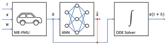
Figure 5.
For NIPT, a single reference simulation with an unchanged is performed to calculate the ANN output for every system state . Based on the recorded ANN inputs and outputs , the actual pre-training can be performed. As soon as the training goal (red-dotted) is reached, the NeuralFMU dynamics equal the dynamics of the FMU itself, which results in the same solution for both. In this case, the ANN’s behavior is neutral.
2.6.2. Collocation Pre-Training (CCPT)
Similar to the collocation training of NeuralODEs [28], collocation training can be performed for NeuralFMUs, too. CCPT is similar to NIPT; the major difference is the training goal (see Figure 6). Whereas NIPT focuses on propagating the unchanged derivatives through the ANN, CCPT aims to hit the derivatives of the ODE solution so that after integration (solving) the target solution can be obtained.
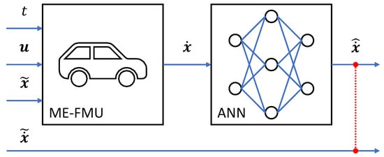
Figure 6.
For CCPT, no reference simulation is performed. For a given state trajectory (e.g., from data), every state is propagated through the FMU and the ANN. As soon as the training goal (red-dotted) is reached, the NeuralFMU dynamics equal the target dynamic (e.g., from data). As a result, the later NeuralFMU solution matches the given state trajectory for a perfect known . The target dynamic may be estimated by deriving and filtering the given system state , or it may be known from measurements.
This method requires knowledge of the entire system state’s trajectory as well as the (at least approximated) state derivative . In general, only a part of the system state and/or derivative of a real system can be measured. Different methods allow for estimating the unknown states, e.g., the Kalman filter [29]. To converge against the target solution, CCPT needs high-quality data on the system state and derivative. Derivatives can be approximated by finite differences or filters (see [28] for an overview). Note that approximating the derivatives may decrease the quality of the pre-training process.
CCPT is only usable if the states of the training objective match the state derivatives manipulated by the ANN. Whereas this is often the case in academic examples, in real applications it is not, which is further exemplified by the VLDM in Section 3.2. To summarize, NIPT does not require the entire state information but converges only against the FMU solution. CCPT, on the other hand, converges against a given target solution but requires a high-fidelity target solution and derivative.
2.6.3. FPM/ANN Gates
The challenge of finding a good initialization by foregoing the pre-training procedure can be bypassed by introducing a slightly modified topology that literally introduces a bypass around the ANN (see Figure 7). The system state derivative is defined as follows, where ∘ stands for the Hadamard product:
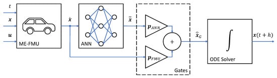
Figure 7.
ME-NeuralFMU with FPM/ANN gates: The ME-FMU receives the current time t and state from the numerical ODE solver together with an external input and computes the corresponding state derivative . Two gates and scale how many dynamic changes by the ANN and the FMU are introduced to the derivative vector . Finally, the derivative vector is passed to the ODE solver with the (adaptive) step size h and integrated into the next system state .
On the one hand, for the case of and , the resulting simulation trajectory is just the simulation trajectory of the original FMU, independent of the ANN parameters. In this way, the NeuralFMU can be initialized without a special initialization routine, while also being capable of manipulating the system dynamics if the parameter is changed to a non-zero value. On the other hand, for the case of and , only the ANN affects the state dynamics, and the original FMU dynamics are used only as the input for the ANN. The parameters and can be optimized along the other training parameters, or, depending on the use case, with a static or dynamic decay/increase. As a final note, CCPT and the FPM/ANN gates’ topology do not exclude each other and can be used together on a NeuralFMU initialization.
2.7. Batching & Training
The training is not performed on the entire data trajectory at one time (e.g., the used CADC Road has a duration of 1001.22 s). Instead, the trajectory is batched. The major challenge at this point is that for a given batch element start time , often only the continuous part of the model state vector of the ME-FMU is known. In general, the discrete part is unknown. As a result, if not explicitly given, a suitable discrete state is determined during the initialization procedure inside the FMU, but it is not guaranteed that this state matches the data and/or expectations. This circumstance also applies to the determination of the initial value of the discrete states , but measurements are often started in a stationary state, where a good understanding of the correct discrete states is given, even if they are not explicitly parts of the data measurements.
As a consequence, training cannot be initialized at an arbitrary element of the batch (time instant) because of the unknown discrete states, which might be initialized unexpectedly if ignored. Estimating the discrete system state on the basis of data is not trivial and may need significant expert knowledge about the model itself. Therefore, a straightforward strategy to handle this is to simulate all batches in the correct order without resetting the FMU between batch elements. Although this does not guarantee the correct discrete state when switching from one batch element to the next during training, the discrete values’ solution converges against the target together with the continuous solution.
Another option is to simulate the entire trajectory for a single time and make memory copies of the entire FMU state using, e.g., fmi2GetFMUstate (in FMI 2.0) at the very beginning of each batch element. This allows for random batches, which might improve the training success and convergence speed. Because the feature required to save and load the FMU memory footprint is optional in FMI and thus often not implemented, this strategy is not further highlighted at this point but can be implemented in a straightforward manner.
Because NeuralFMUs are a subclass of NeuralODEs, in addition to the ones mentioned, many techniques for NeuralODEs can be adapted to improve the training process in terms of stability and convergence, such as, for example, multiple shooting, as in [30].
3. Results
The considered method is validated in the following application: Based on the introduced VLDM, a hybrid model is deployed leading to a significantly better consumption prediction than the original FPM. Even if the FPM already considers multiple friction effects, it is assumed that the prediction error is the result of a wrongly parameterized, or an additional, non-modeled friction effect. The goal is to inject an additional vehicle acceleration to force the driver controller to perform a higher engine torque thus increasing the vehicle energy consumption. References for the used open-source software, data and (soon) a tutorial replicating the presented results are available at the URLs provided in the Data Availability Statement.
3.1. Example Model: Vehicle Longitudinal Dynamics Model (VLDM)
In this section, the used FMU model is introduced. The model represents the longitudinal dynamics of an electric Smart EQ fortwo and is an adaption of a model from the Technical University of Munich [31]. In automotive applications, longitudinal dynamics models are often used to simulate energy consumption; thus, only the related effects are represented in the model. The original model was created in MATLAB®/Simulink®, replicated analogously in the modeling language Modelica® and exported as an FMU. The following Figure 8 shows the topology of the simulation model. The full vehicle model is modular and consists of six core components [32].
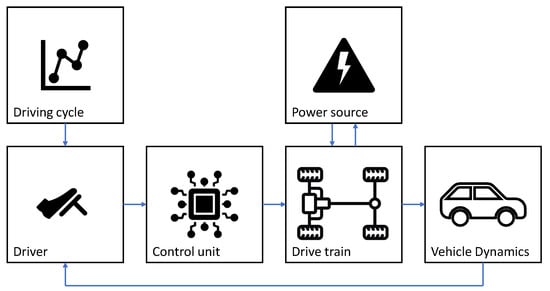
Figure 8.
Topology of the VLDM (own representation adapted from [31]).
The top-layer components of the vehicle are the Driving cycle, the Driver, the Control unit, the Power source, the Drive train and the Vehicle dynamics subsystems. The target vehicle speed, read from a driving cycle tabular in the Driving cycle subsystem, is forwarded to the Driver. The Driver consists of two PI-controllers for the acceleration and brake pedal, which make the vehicle follow the given driving cycle. The block Control unit calculates the desired torque from the pedal position. The required power is provided by the Power source component, modeling the vehicle battery. In the Drive train block, the sources of acceleration and braking torques are implemented. This component contains the electric motor, the power electronics, the transmission and the tire models. In the component Vehicle dynamics, the rolling, air and slope resistances are implemented. The resulting force and torque determine the acceleration of the vehicle, and, after numerical integration, the speed and position [31]. Finally, the vehicle speed is fed back into the Driver subsystem and closes the controller loop. Together with the model itself, multiple measurements from an automotive driving test rig with different driving cycles, such as the Common Artemis Driving Cycles (CADC), New European Driving Cycle (NEDC) and Worldwide Harmonized Light-Duty Vehicles Test Cycle (WLTC), were published [33]. We use the driving cycles CADC Road and WLTC Class 2 for the presented experiment.
The simulation model counts six continuous states in total:
- the PI-controller state (integrated error) for the throttle pedal (Driver);
- the PI-controller state (integrated error) for the brake pedal (Driver);
- the integrated driving cycle speed and the cycle position (Driving cycle);
- the vehicle position (Vehicle dynamics);
- the vehicle velocity (Vehicle dynamics);
- the cumulative consumption (energy).
Analogous, the six continuous state derivatives are:
- the PI-controller error/deviation for the throttle pedal (Driver);
- the PI-controller error/deviation for the brake pedal (Driver);
- the driving cycle speed (Driving cycle);
- the vehicle velocity (Vehicle dynamics);
- the vehicle acceleration (Vehicle dynamics);
- the current consumption (power).
Note that this system features different challenging attributes, such as:
- The system is highly discontinuous, meaning it has a significant amount of explicitly time-dependent events (100 events per second). This further limits the maximum time step size for the numerical solver and therefore worsens the simulation and training performance;
- The simulation contains a closed-loop over multiple subsystems with two controllers running at 100 Hz (the source of the high-frequency time events);
- The system contains a large amount of state-dependent events, triggered by 22 event indicators;
- Measurements of the real system are not equidistant in time (even if it was saved this way, which introduces a typical measurement error);
- Only a subpart of the system state vector is part of the measurements, the remaining parts are estimated;
- The measurements are not exact and contain typical, sensor- and filter-specific errors (such as noise and oscillation);
- There is a hysteresis loop for the activation of the throttle and brake pedal. The PI-controller states are initialized at corresponding edges of the hysteresis loop;
- The system is highly non-linear, e.g., multiple quantities are saturated;
- Characteristic maps (data models) for the electric power, inverted electric power and the electric power losses are used.
Combining all of these attributes results in a challenging FPM for the considered hybrid modeling use case.
3.2. Topology
Combining the original NeuralFMU topology (Figure 3) with pre- and post-processing (Section 2.5) and FPM/ANN gates (Section 2.6.3) results in the topology shown in Figure 9, which is used for training the hybrid model in the considered use case.
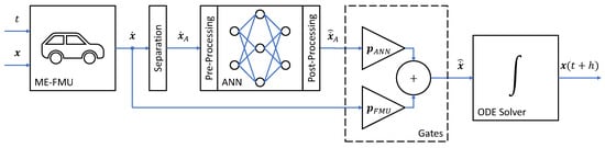
Figure 9.
Topology of the used ME-NeuralFMU: The ME-FMU receives the current time t and state from the numerical ODE solver and computes the corresponding state derivative . The state derivative is then trimmed to a subset of derivatives . Before the ANN transforms , the signals are pre-processed to approximately fit a standard normal distribution. After the ANN’s inference, the inverse transformation of the pre-process is applied to the post-processed, and is obtained. Two gates and scale how much and are introduced to the final derivative vector . Finally, the changed derivative vector is passed to the ODE solver with the (adaptive) step size h and integrated into the next system state . The used FMU has no continuous inputs ; the driving cycle is part of the model and depends only on the time t.
In general, understanding at least some aspects of the physical effect, which is to be modeled by the ANNs, is a great advantage. Basically, any value of the FMU that is accessible via the FMI can be used as the input for the ANNs: the system states and derivatives, system inputs and any other system variable (or output) that depends on the system state, input and/or time. This allows for a wide variety of NeuralFMU topologies. However, using all available variables in the interface to the ANNs can result in suboptimal training performance because more variable sensitivities need to be determined and signals without physical dependency can be misinterpreted as dependent. This motivates the use of a clever, minimal subset of the available FMU variables. Often, state and state derivatives are good choices for variables to feed into the ANN because from a mathematical point of view, the system state holds all relevant information in a minimal representation. Nevertheless, the addition of more variables may be productive, even if the encapsulated system information is redundant. This is purposeful, if the correlations between the training objective and these additional variables are easier to fit for an ANN than the correlation with system states and/or derivatives.
For the considered use case, a friction effect is learned. Conventional mechanical friction models, such as viscous damping or slip–stick friction, often depend on the physical body’s translational or rotational velocity. Therefore, the vehicle speed in particular should be considered. Further, the current vehicle acceleration and power are also given as inputs to the ANN. The training objective is to match the cumulative consumption from the training data by manipulating the vehicle acceleration. Here, CCPT cannot be used because the CCPT objective would be to fit the cumulative consumption derivative, i.e., the current consumption, but this value is not directly affected by the ANN.
To summarize, the following variables (compare to Figure 9) are used:
- corresponds to the vehicle speed, acceleration and power (current consumption). These are the inputs for the ANN;
- corresponds to the estimated vehicle acceleration by the ANN. This is the output of the ANN (technically, it is the only output because the other five dynamics are assumed always to be zero and are neglected);
- . Only the influence of the vehicle acceleration from the ANN can be controlled via (this is the only ANN output);
- . Only the influence of the vehicle acceleration from the FMU can be controlled via (all other derivatives contribute 100%).
Note that if the considered effect depends on the system states, then states can also be passed as the input to the ANN. Because the hybrid model reuses the FPM, and therefore the ANN only needs to approximate the unmodeled physical effect, a very lightweight net layout is sufficient, as shown in Table 1. This results in fast training because of the small number of parameters.

Table 1.
ANN layout and parameters of the used topology.
3.3. Consumption Prediction
As already mentioned, the model is validated by comparing the most important simulation value (quantity of interest) to the measurement data: The cumulative consumption of the vehicle over the entire driving cycle.
3.3.1. Training
After training of 18 epochs on the CADC Road with a batch element length of 100 s, resulting in 11 batch elements, the NeuralFMU is able to outperform the FPM on training data (see Figure 10, Figure 11 and Figure 12). The following figures show the predicted cumulative consumption over time of the original FPM compared to the trained NeuralFMU. The training is not converged at this point. The cost function is implemented as an ordinary MSE between the data and predicted cumulative consumption. For parameter optimization, we use Adam [34] with an exponential decay (initial step size: , decay (new step size multiplier): every step, min. step size: ). The training is performed single-core on a CPU (Intel® CoreTM i7-8565U on Windows 10 Enterprise 20H2) and takes ≈5 h. During interpretation of the results, note the small amount of data used for training: a single driving cycle measurement trajectory (mean over two real experiments).
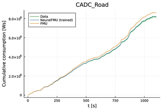
Figure 10.
Cumulative consumption prediction on the CADC Road, which is part of the training data. The NeuralFMU (blue) lies almost on the training data mean (green) and inside the data uncertainty region (green, translucent). On the other hand, the simulation results of the original FPM/FMU (orange) slowly drifts out of the data uncertainty region, resulting in a relatively large error at the simulation stop time compared to the NeuralFMU.
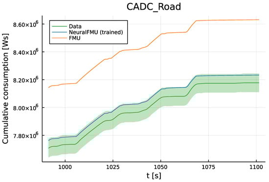
Figure 11.
Deviation on the last 10% of the cumulative consumption prediction on the CADC Road, which is part of the training data. The final consumption prediction accuracy of the NeuralFMU (blue) significantly increases compared to the original FMU (orange), lies inside the measurement uncertainty (green, translucent) and close to the data’s mean (green). The original FPM prediction lies completely outside of the measurement uncertainty.
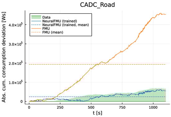
Figure 12.
Deviation (absolute error) of the consumption prediction between data and the NeuralFMU (blue) compared to the original FPM/FMU (orange) on the CADC Road, which is part of the training data. After ≈300 s, the NeuralFMU solution lies inside the data uncertainty region (green, translucent) and outperforms the FPM in terms of prediction accuracy. Further, the NeuralFMU error is at any time step significantly smaller than the mean error of the FMU (orange, dashed).
3.3.2. Testing (Validation)
After training, the NeuralFMU is validated against unknown data by simulating another driving cycle, the WLTC Class 2, which is not known from training. This is challenging, because the WLTC Class 2 (mean: m/s, max: m/s) features a very different speed profile compared to the CADC Road (mean: m/s, max: m/s). This especially includes higher velocities that are not part of the training data, which is a good test for the extrapolation capabilities of the hybrid model. Results and explanations can be seen in Figure 13, Figure 14 and Figure 15.
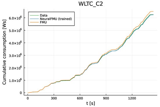
Figure 13.
Comparison of the cumulative consumption prediction, using the WLTC Class 2, which is not part of the NeuralFMU training data. As for the training data, the NeuralFMU prediction (blue) is closer to the measurement data mean (green) than the original FPM prediction (orange).
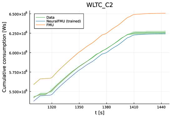
Figure 14.
Deviation on the last 10% of the simulation trajectory of the NeuralFMU (blue) compared to the original FPM/FMU (orange) and experimental data mean (green). The unknown WLTC Class 2 is used for testing. The NeuralFMU prediction is much closer to the data mean than the original FPM and predicts a final value inside of the measurement uncertainty.
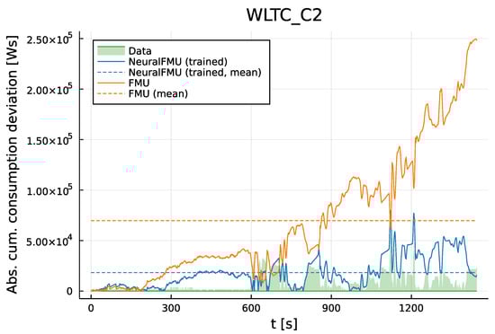
Figure 15.
Absolute error of the consumption prediction of the NeuralFMU (blue) compared to the original FPM/FMU (orange). The unknown WLTC Class 2 is used for testing. Even if the NeuralFMU solution (blue) does not always lie inside the data uncertainty region (green), it leads to a much better prediction than the original FPM, which, in contrast, almost completely misses the data uncertainty area (green, translucent).
For training as well as for testing data, the NeuralFMU solution leads to a smaller MSE, maximum error and final error than the solution of the original FPM. For the training cycle, the NeuralFMU solution proceeds inside of the measurement uncertainty, which is a great success. Moreover, for testing data, the NeuralFMU increases prediction accuracy compared to the FPM but leaves the data uncertainty region in some sections. A detailed overview of the training and testing results can be seen in Table 2.
Table 2.
Training and testing results with solver Tsit5 after 18 training epochs. Errors are calculated against the data mean of two chassis dynamometer runs.
Because longitudinal dynamics models are often used to predict the cumulative consumption on entire cycles, the final value of the solution is especially important and a key factor for model evaluation. Note that this final error of the NeuralFMU is over 8 times smaller on the training data and even 16 times smaller on the validation data. In addition to the final error, the NeuralFMU features a much lower MSE (factor ≈ 63 on training, factor ≈ 16 on testing) and maximum error (factor ≈ 7 on training, factor ≈ 3 on testing), but the simulation time increases about five or six times. This is mainly because of the more expensive event handling inside the hybrid structure and the additional unused performance optimizations in the prototypical implementation. It can be seen that the number of events remains unchanged. The number of adaptive solver steps only slightly increases, which indicates that the average system stiffness hardly changes. Here, an ODE is considered stiff if the adaptive step size of the solver is controlled authoritatively by the stability objective instead of the tolerance objective. Finally, the training is not converged yet and further training epochs or training on more data (e.g., multiple cycles) may reduce the remaining deviations.
4. Conclusions
We highlighted a workflow to allow for hybrid modeling on basis of an industry-typical FPM in the form of a NeuralFMU. Before training such models, a proper initialization is required. Because initialization of NeuralFMUs is not trivial, we suggest three methods with different requirements: NIPT, CCPT and a topology using the ANN/FMU gates, which makes an initialization routine obsolete. The use of this topology was tested in practice using an industry-typical FPM, the VLDM. This model features multiple challenges, such as closed loops and high-frequency discontinuities. The VLDM was exported in a format that is common in industrial practice, the FMI. On the foundation of the exported FMU, a hybrid model was built and trained on real measurement data from a chassis dynamometer, including typical measurement errors. The model was trained on only a single driving cycle measurement to show that the presented method is capable of making good predictions on very little data. The trained hybrid model was able to make better predictions compared to the FPM on both the training and testing data. To check the training success for overfitting, another driving cycle was simulated, also featuring better results than the original FPM. To conclude, the presented workflow and software allow for the reuse of existing industrial models as cores of NeuralFMUs, which can surpass the prediction quality of the original FPM. Using the presented methodology, NeuralFMUs allow for data-driven modeling of physical effects that are difficult to model based on the first principle.
On the software side, we briefly introduced two Julia libraries. First, the FMUs are imported into Julia using FMI.jl, where they can be further parameterized and simulated. Using FMIFlux.jl, a NeuralFMU can be set up based on any FMU as easily as setting up a conventional deep ANN. After creation, the NeuralFMU can be trained, including proper event handling for discontinuous systems. Finally, FMIFlux.jl makes continuous and discontinuous FMUs differentiable, therefore opening up a variety of hybrid modeling use cases in addition to NeuralFMUs.
Because the presented work concerns ME-FMUs, which can be seen as containers for ODEs, the highlighted methods are not limited to automotive use cases but open up to basically any system that can be represented as system of ODEs. Further, PDEs (e.g., in fluid dynamic simulations) can be spatially discretized to obtain ODEs for use as the core of a NeuralFMU, as shown in our work in [10]. Moreover, DAEs can be used after model order reduction into an ODE. This allows for a wide variety of use cases in different domains, such as medical sciences, biology and chemistry, or as presented in mechatronic systems, as in the automotive industry. Even the use of a NeuralFMU as part of system control, for example, in the field of model-based control is conceivable.
The library repositories are constantly expanded upon by new features and maintained for upcoming technological progress. Contributors are welcome.
Author Contributions
Conceptualization, T.T. and L.M.; methodology, T.T. and L.M.; software, T.T. and L.M.; validation, T.T., J.S. and L.M.; first-principle model: J.S., L.M. and T.T.; writing—original draft preparation, T.T., J.S. and L.M.; writing—review and editing, T.T., J.S. and L.M.; visualization, T.T. and L.M. All authors have read and agreed to the published version of the manuscript.
Funding
This research was partially funded by the ITEA3-Project UPSIM (Unleash Potentials in Simulation) Nr. 19006. For more information, see: (https://www.upsim-project.eu/ (accessed on
28 September 2022)).
Institutional Review Board Statement
Not applicable.
Informed Consent Statement
Not applicable.
Data Availability Statement
The used software FMI.jl and FMIFlux.jl are available open-source at https://github.com/ThummeTo/FMI.jl, (accessed on 28 September 2022) and https://github.com/ThummeTo/FMIFlux.jl, (accessed on 28 September 2022). The data used in the presented experiment (vehicle measurements) as well as the original model are available for download at https://github.com/TUMFTM/Component_Library_for_Full_Vehicle_Simulations, (accessed on 28 September 2022). Further, a tutorial for reconstruction of the presented method focusing on adapting custom use cases will be released soon after this article’s publication in the repository of FMIFlux.jl.
Acknowledgments
The authors thank everyone that contributed to the library repositories, especially our students and student assistants Josef Kircher, Jonas Wilfert and Adrian Brune.
Conflicts of Interest
The authors declare no conflict of interest.
Abbreviations
The following abbreviations are used in this manuscript:
| AD | Automatic Differentiation |
| ANN | Artifical Neural Networks |
| BNSDE | Bayesian Neural Stochastic Differential Equations |
| CADC | Common Artemis Driving Cycles |
| CCPT | Collocation Pre-Training |
| CS | Co-Simulations |
| DAE | Differential-Algebraic Systems of Equations |
| DARN | Deep Auto-Regressive Networks |
| FMI | Functional Mock-up Interface |
| FMU | Functional Mock-up Unit |
| FPM | First-Principle Models |
| HiL | Hardware in the Loop |
| ME | Model Exchange |
| ML | Machine Learning |
| MSE | Mean Squared Error |
| NEDC | New European Driving Cycle |
| NIPT | Neutral Initialization Pre-Training |
| ODE | Ordinary Differential Equation |
| PAC | Probably Approximately Correct |
| PDE | Partial Differential Equations |
| PINN | Physics-Informed Neural Network |
| RNN | Recurrent Neural Network |
| SE | Scheduled Execution |
| SSP | System Structure and Parameterization |
| VLDM | Vehicle Longitudinal Dynamics Model |
| WLTC | Worldwide Harmonized Light-Duty Vehicles Test Cycle |
References
- Raissi, M.; Perdikaris, P.; Karniadakis, G. Physics-informed neural networks: A deep learning framework for solving forward and inverse problems involving nonlinear partial differential equations. J. Comput. Phys. 2019, 378, 686–707. [Google Scholar] [CrossRef]
- Haussmann, M.; Gerwinn, S.; Look, A.; Rakitsch, B.; Kandemir, M. Learning Partially Known Stochastic Dynamics with Empirical PAC Bayes. arXiv 2021, arXiv:cs.LG/2006.09914. [Google Scholar]
- Gregor, K.; Danihelka, I.; Mnih, A.; Blundell, C.; Wierstra, D. Deep AutoRegressive Networks. ACM Digit. Libr. 2013, 32, 242–250. [Google Scholar] [CrossRef]
- Bruder, F.; Mikelsons, L. Modia and Julia for Grey Box Modeling. In Proceedings of the 14th Modelica Conference 2021, Linköping, Sweden, 20–24 September 2021; pp. 87–95. [Google Scholar] [CrossRef]
- Rai, R.; Sahu, C.K. Driven by Data or Derived Through Physics? A Review of Hybrid Physics Guided Machine Learning Techniques With Cyber-Physical System (CPS) Focus. IEEE Access 2020, 8, 71050–71073. [Google Scholar] [CrossRef]
- Willard, J.; Jia, X.; Xu, S.; Steinbach, M.; Kumar, V. Integrating Physics-Based Modeling with Machine Learning: A Survey. arXiv 2020, arXiv:physics.comp-ph/2003.04919. [Google Scholar]
- Chen, T.Q.; Rubanova, Y.; Bettencourt, J.; Duvenaud, D. Neural Ordinary Differential Equations. arXiv 2018, arXiv:1911.07532. [Google Scholar]
- Innes, M.; Edelman, A.; Fischer, K.; Rackauckas, C.; Saba, E.; Shah, V.B.; Tebbutt, W. A Differentiable Programming System to Bridge Machine Learning and Scientific Computing. arXiv 2019, arXiv:1907.07587. [Google Scholar]
- Thummerer, T.; Mikelsons, L.; Kircher, J. NeuralFMU: Towards structural integration of FMUs into neural networks. In Proceedings of the 14th Modelica Conference 2021, Linköping, Sweden, 20–24 September 2021. [Google Scholar] [CrossRef]
- Thummerer, T.; Tintenherr, J.; Mikelsons, L. Hybrid modeling of the human cardiovascular system using NeuralFMUs. J. Phys. Conf. Ser. 2021, 2090, 012155. [Google Scholar] [CrossRef]
- Modelica Association. Homepage of the FMI-Standard. Available online: https://fmi-standard.org/ (accessed on 28 September 2022).
- Modelica Association. Functional Mock-Up Interface for Model Exchange and Co-Simulation, Document Version: 2.0.2; Technical Report; Modelica Association: Linköping, Sweden, 2020. [Google Scholar]
- Modelica Association. Functional Mock-Up Interface Specification, Document Version: 3.0; Technical Report; Modelica Association: Linköping, Sweden, 2022. [Google Scholar]
- Modelica Association. System Structure and Parameterization, Document Version: 1.0; Technical Report; Modelica Association: Linköping, Sweden, 2019. [Google Scholar]
- SciML, Julia Computing. DiffEqFlux.jl Repository on GitHub. Available online: https://github.com/SciML/DiffEqFlux.jl (accessed on 28 September 2022).
- Rackauckas, C.; Innes, M.; Ma, Y.; Bettencourt, J.; White, L.; Dixit, V. DiffEqFlux.jl-A Julia Library for Neural Differential Equations. arXiv 2019, arXiv:1902.02376. [Google Scholar]
- Bezanson, J.; Edelman, A.; Karpinski, S.; Shah, V.B. Julia: A Fresh Approach to Numerical Computing. arXiv 2015, arXiv:1411.1607. [Google Scholar] [CrossRef]
- Revels, J.; Lubin, M.; Papamarkou, T. Forward-Mode Automatic Differentiation in Julia. arXiv 2016, arXiv:1607.07892. [Google Scholar]
- Revels, J.; Papamarkou, T.; Lubin, L.; Other Contributors. Available online: https://github.com/JuliaDiff/ForwardDiff.jl (accessed on 28 September 2022).
- Innes, M. Don’t Unroll Adjoint: Differentiating SSA-Form Programs. arXiv 2018, arXiv:1810.07951. [Google Scholar]
- Julia Computing, Inc.; Innes, M.J.; Other Contributors. Zygote.jl Repository on GitHub. Available online: https://github.com/FluxML/Zygote.jl (accessed on 28 September 2022).
- Elmqvist, H.; Neumayr, A.; Otter, M. Modia-Dynamic Modeling and Simulation with Julia. In Proceedings of the Juliacon 2018, London, UK, 26 November 2018; Available online: https://elib.dlr.de/124133/ (accessed on 28 September 2022).
- Elmqvist, H.; DLR Institute of System Dynamics and Control. Modia.jl Repository on GitHub. Available online: https://github.com/ModiaSim/Modia.jl (accessed on 28 September 2022).
- Thummerer, T.; Mikelsons, L.; Kircher, J.; Other Contributors. FMI.jl Repository on GitHub. Available online: https://github.com/ThummeTo/FMI.jl (accessed on 28 September 2022).
- Thummerer, T.; Mikelsons, L. FMIFlux.jl Repository on GitHub. Available online: https://github.com/ThummeTo/FMIFlux.jl (accessed on 28 September 2022).
- Julia Computing, Inc.; Innes, M.J.; Other Contributors. Flux.jl Repository on GitHub. Available online: https://github.com/FluxML/Flux.jl (accessed on 28 September 2022).
- Gorecki, S.; Possik, J.; Zacharewicz, G.; Ducq, Y.; Perry, N. A Multicomponent Distributed Framework for Smart Production System Modeling and Simulation. Sustainability 2020, 12, 6969. [Google Scholar] [CrossRef]
- Roesch, E.; Rackauckas, C.; Stumpf, M. Collocation based training of neural ordinary differential equations. Stat. Appl. Genet. Mol. Biol. 2021, 20, 25. [Google Scholar] [CrossRef]
- Kalman, R.E. A New Approach to Linear Filtering and Prediction Problems. J. Basic Eng. 1960, 82, 35–45. [Google Scholar] [CrossRef]
- Turan, E.M.; Jäschke, J. Multiple Shooting for Training Neural Differential Equations on Time Series. IEEE Control Syst. Lett. 2022, 6, 1897–1902. [Google Scholar] [CrossRef]
- Danquah, B.; Koch, A.; Weis, T.; Lienkamp, M.; Pinnel, A. Modular, Open Source Simulation Approach: Application to Design and Analyze Electric Vehicles. In Proceedings of the IEEE 2019 Fourteenth International Conference on Ecological Vehicles and Renewable Energies (EVER), Monte Carlo, Monaco, 8–10 May 2019; pp. 1–8. [Google Scholar] [CrossRef]
- Guzzella, L.; Sciarretta, A. Vehicle Propulsion Systems: Introduction to Modeling and Optimization, 3rd ed.; Springer: Berlin/Heidelberg, Germany, 2013. [Google Scholar]
- Danquah, B. Component Library for Full Vehicle Simulations Repository on GitHub. Available online: https://github.com/TUMFTM/Component_Library_for_Full_Vehicle_Simulations (accessed on 28 September 2022).
- Kingma, D.P.; Ba, J. Adam: A Method for Stochastic Optimization. arXiv 2014, arXiv:1412.6980. [Google Scholar]


Publisher’s Note: MDPI stays neutral with regard to jurisdictional claims in published maps and institutional affiliations. |
© 2022 by the authors. Licensee MDPI, Basel, Switzerland. This article is an open access article distributed under the terms and conditions of the Creative Commons Attribution (CC BY) license (https://creativecommons.org/licenses/by/4.0/).