
Analysis of Electric Energy Consumption Profiles Using a Machine Learning Approach: A Paraguayan Case Study

 ,
,  , , , ,
  ,
,  , , , ,
  and
and
Abstract
:1. Introduction
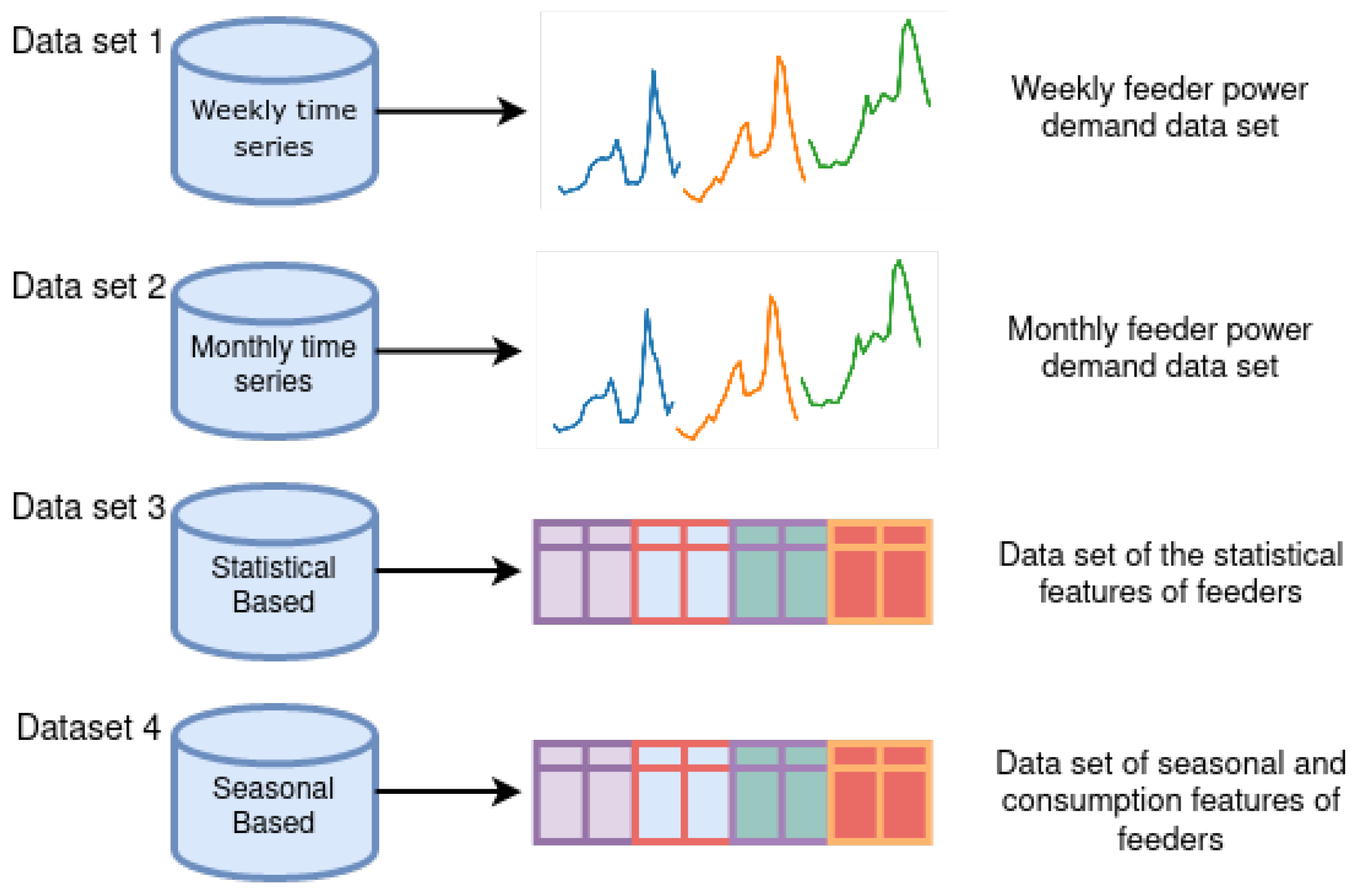
- Weekly time series data, where the consumption of each feeder was aggregated on a weekly basis;
- Monthly time series data, where the consumption of each feeder was aggregated on a monthly basis;
- Statistical data set—a set of statistical features was calculated from the raw data;
- Seasonal and daily load curve feature data set—a set of features based on the daily load curve and seasonal consumption variations was computed.
- Analysis and comparison of the performance of different clustering algorithms using real electricity consumption data collected from a Paraguayan electricity provider.
- Study of the suitability of four different data processing strategies.
- Evaluation of the influence of distance metrics and linkage criteria for this particular case study.
2. Related Works
3. Materials and Methods
3.1. Data
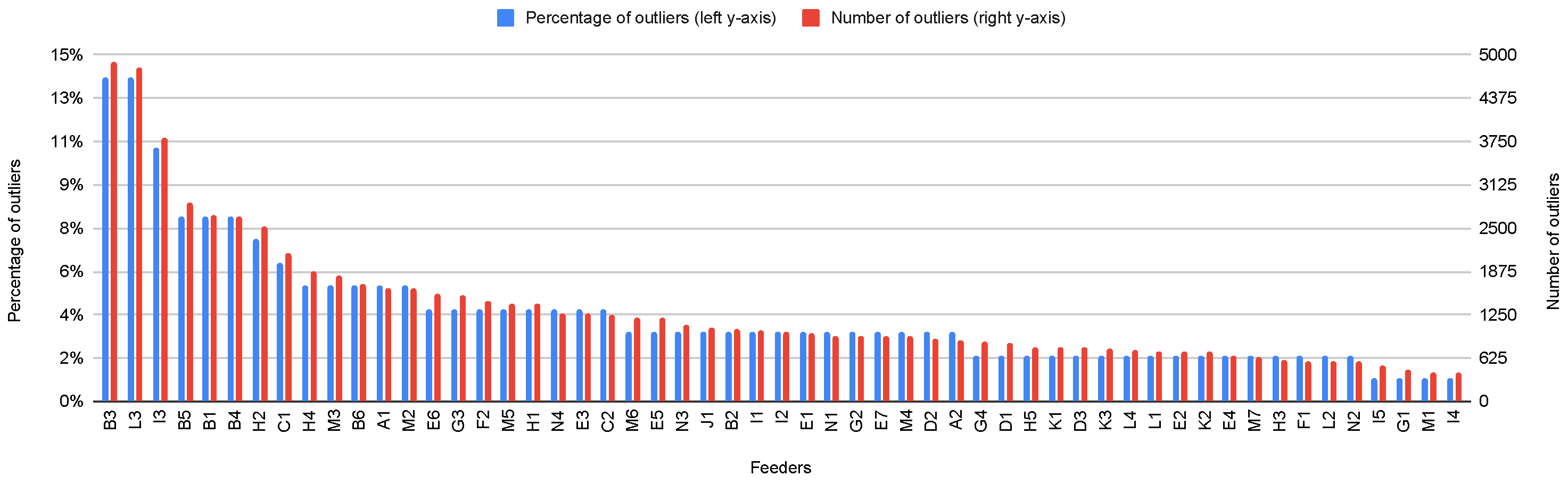
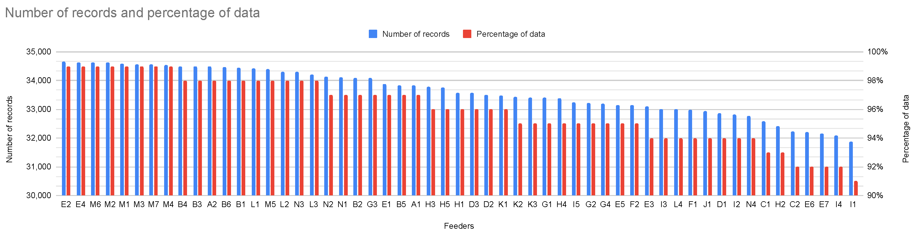
3.2. Data Preprocessing
3.3. Data Sets and Features
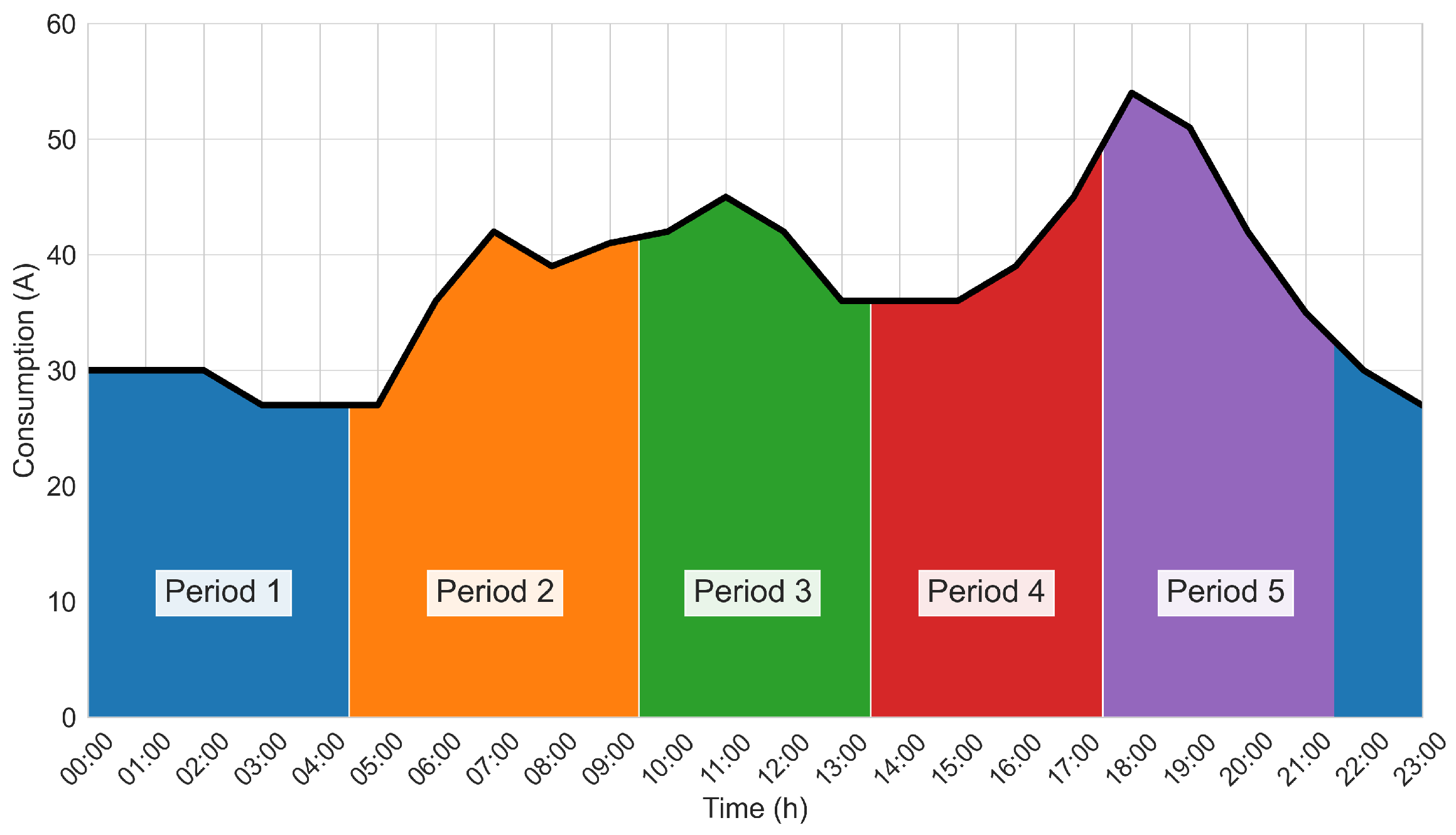
- Features from 1 to 5: The relative average power in each time period over the entire time series given by
- Feature 6: Mean relative standard deviation over the entire time series given by
- Feature 7: A seasonal score given by
- Feature 8: A weekend vs. weekday difference score given by
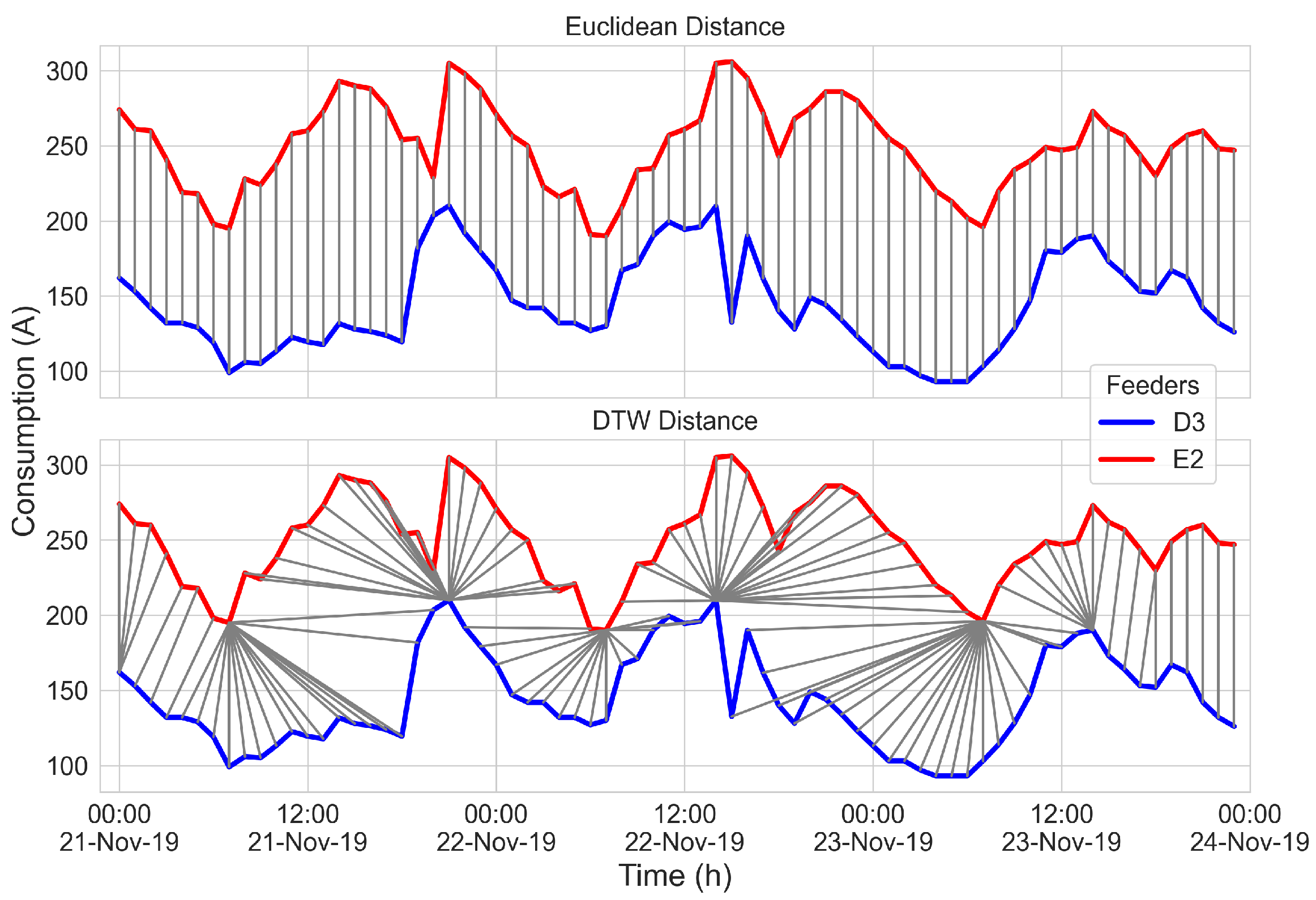
3.4. Distance Measurements
3.5. Clustering Techniques
3.5.1. K-Means
3.5.2. Hierarchical Clustering
3.5.3. K-Spectral Centroid
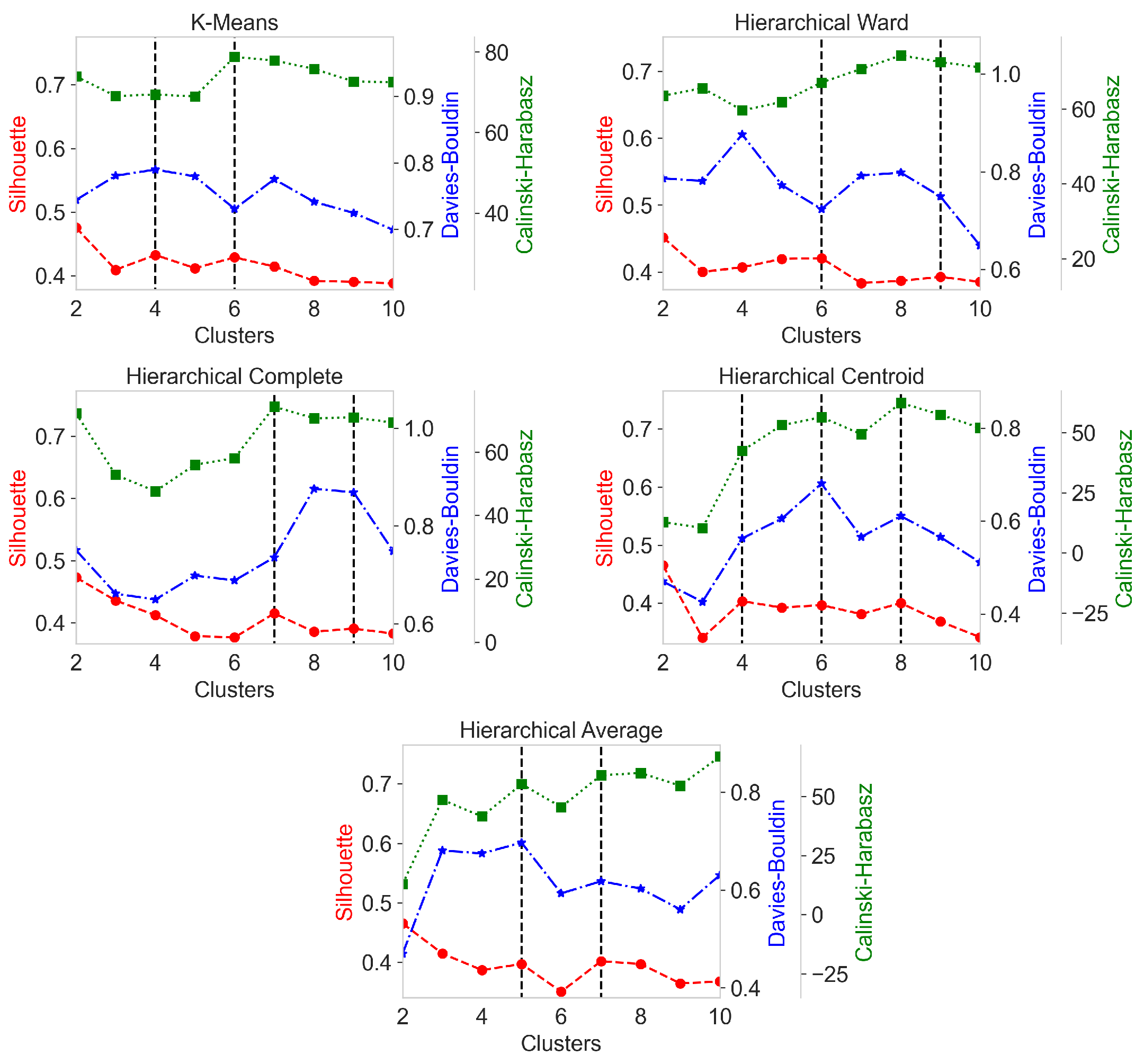
3.6. Cluster Validity Indices
3.7. Workflow
4. Results
- Comparison of the different clustering techniques studied to identify the best models according to the cluster validity index measures.
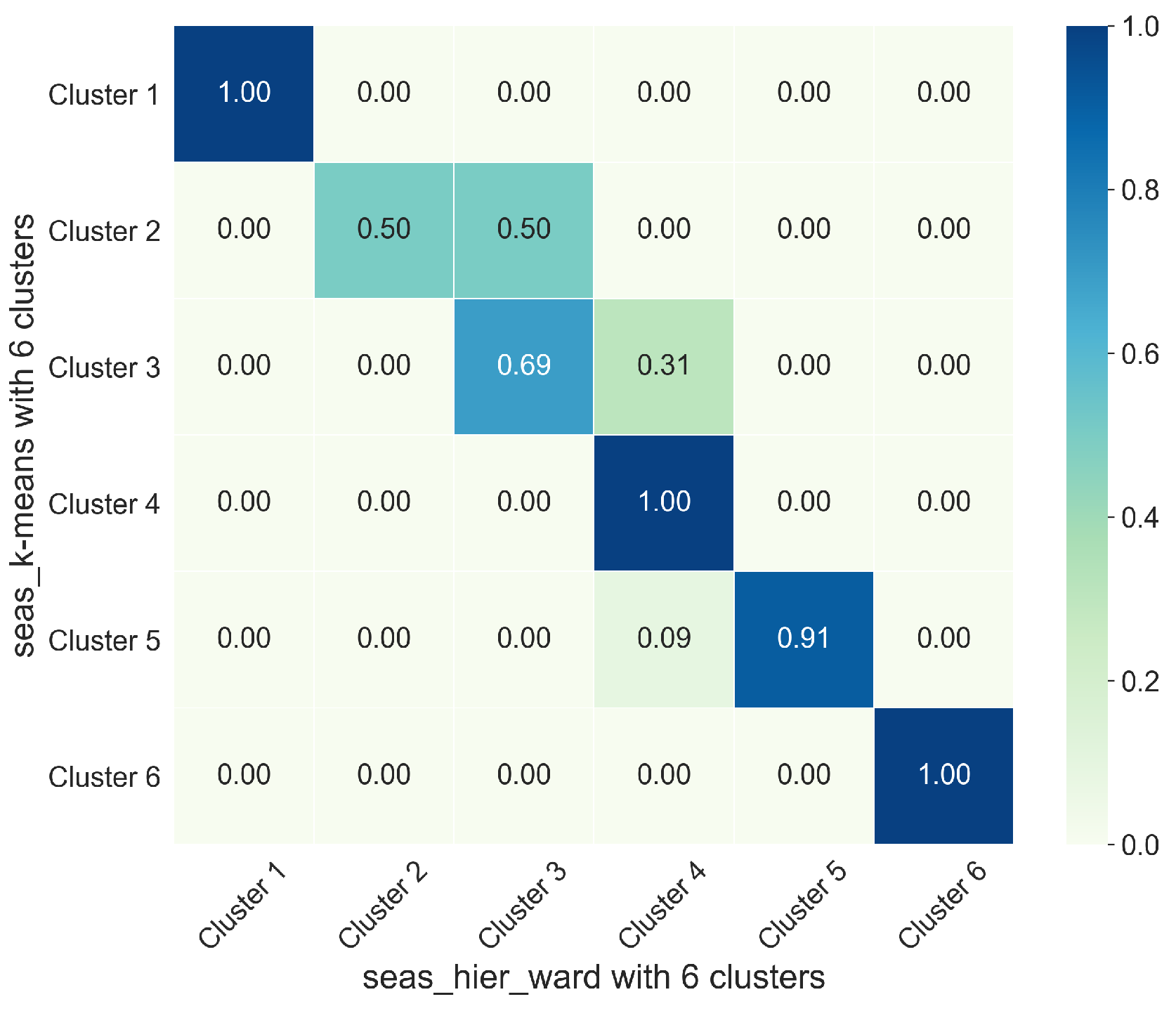
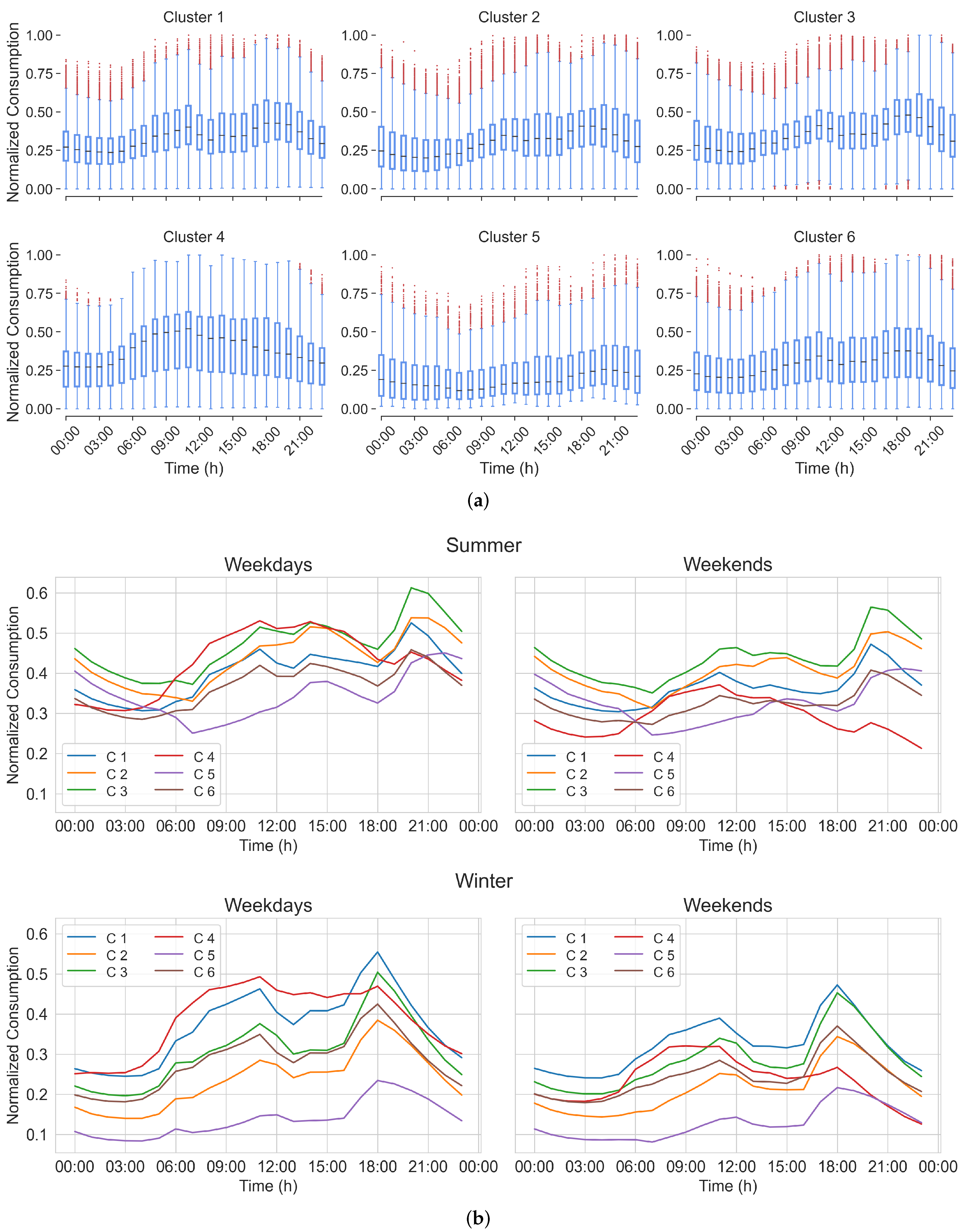
- Analysis of the consumption data of the best model found.l.
4.1. Model Comparison
4.2. Analysis of Selected Model
5. Discussion
Author Contributions
Funding
Data Availability Statement
Acknowledgments
Conflicts of Interest
List of Symbols
| Symbol | Description |
| Time series | |
| Box–Cox transformation of time series | |
| Seasonal component of time series | |
| Trend component of time series | |
| Remainder component of time series | |
| Historical records where DOW is the same as the one on the missing record | |
| Mean | |
| Standard deviation | |
| Skewness | |
| Kurtosis | |
| Initial separation vector | |
| Separation vector | |
| Maximum Lyapunov exponent | |
| Period | |
| Periodicity | |
| Power spectral density | |
| Energy | |
| P | Mean electricity demand |
| Mean daily demand over a complete time series | |
| Mean summer demand | |
| Mean winter demand | |
| Mean weekday demand | |
| Mean weekend demand | |
| Relative average power | |
| Mean relative standard deviation | |
| Seasonal score | |
| Weekend vs. weekday difference score | |
| Set of objects | |
| Size of a set of objects | |
| C | Cluster |
| c | Centroid of a cluster |
| E | Sum of squared distances between objects and their centroid in all clusters |
| Euclidean distance | |
| Dynamic time warping distance | |
| M | Cost matrix for DTW |
| Optimal warping path | |
| Cost function for DTW | |
| Average distance of a sample with respect to the others in the same cluster | |
| Average distance of the same sample with respect to those in the nearest cluster | |
| ⟆ | Silhouette index for a sample |
| Average score of the Silhouette index (Silhouette index) | |
| Average distance between the centroid of a considered cluster and the objects that conform it | |
| Distance between centroids of two clusters | |
| R | Similarity score between clusters |
| Davies–Bouldin index | |
| B | Between-cluster dispersion matrix |
| W | Within-cluster dispersion matrix |
| Calinski–Harabasz index |
Abbreviations
| DNOs | Distribution network operators |
| DWT | Discrete wavelet transform |
| NN | Neural networks |
| SVM | Support vector machine |
| DTW | Dynamic time warping |
| LD | Linear dichroism |
| DOW | Day of the week |
| MLE | Maximum Lyapunov exponent |
| FFT | Fast Fourier transform |
References
- Schneider, K.P.; Chen, Y.; Engle, D.; Chassin, D. A taxonomy of North American radial distribution feeders. In Proceedings of the IEEE Power & Energy Society General Meeting, Calgary, AB, Canada, 26–30 July 2009; pp. 1–6. [Google Scholar]
- Jneid, J. Cluster Analysis for Medium Voltage Distribution Feeders; McGill University: Montreal, QC, Canada, 2020. [Google Scholar]
- Bernards, R.; Morren, J.; Slootweg, H. Incorporating the smart grid concept in network planning practices. In Proceedings of the 2015 50th International Universities Power Engineering Conference (UPEC), Stoke-on-Trent, UK, 1–4 September 2015; pp. 1–5. [Google Scholar]
- Parada, V.; Ferland, J.A.; Arias, M.; Daniels, K. Optimization of electrical distribution feeders using simulated annealing. IEEE Trans. Power Deliv. 2004, 19, 1135–1141. [Google Scholar] [CrossRef]
- Collin, A.J.; Tsagarakis, G.; Kiprakis, A.E.; McLaughlin, S. Development of low-voltage load models for the residential load sector. IEEE Trans. Power Syst. 2014, 29, 2180–2188. [Google Scholar] [CrossRef]
- Agner, F. Creating Electrical Load Profiles Through Time Series Clustering; Technical Report for Lund University: Lund, Sweden, 2019. [Google Scholar]
- Ullón, H.R.; Ugarte, L.F.; Lacusta, E., Jr.; de Almeida, M.C. Characterization of load curves in a real distribution system based on K-MEANS algorithm with time-series data. In Proceedings of the Congresso Brasileiro de Automática-CBA, Gramado, Brazil, 12 September 2020; Volume 2. [Google Scholar]
- Panapakidis, I.; Alexiadis, M.; Papagiannis, G. Load profiling in the deregulated electricity markets: A review of the applications. In Proceedings of the 9th International Conference on the European Energy Market, Piscataway, NJ, USA, 10–12 May 2012; pp. 1–8. [Google Scholar]
- Scarlatache, F.; Grigoraş, G.; Chicco, G.; Cârţină, G. Using k-means clustering method in determination of the optimal placement of distributed generation sources in electrical distribution systems. In Proceedings of the 13th International Conference on Optimization of Electrical and Electronic Equipment (OPTIM), Brasov, Romania, 24–26 May 2012; pp. 953–958. [Google Scholar]
- Lee, E.; Kim, J.; Jang, D. Load profile segmentation for effective residential demand response program: Method and evidence from Korean pilot study. Energies 2020, 13, 1348. [Google Scholar]
- Sakoe, H.; Chiba, S. Dynamic programming algorithm optimization for spoken word recognition. IEEE Trans. Acoust. Speech, Signal Process. 1978, 26, 43–49. [Google Scholar] [CrossRef] [Green Version]
- Velázquez, G.; Morales, F.; García-Torres, M.; Gómez-Vela, F.; Divina, F.; Vázquez Noguera, J.; Daumas-Ladouce, F.; Sauer Ayala, C.; Pinto-Roa, D.P.; Gardel-Sotomayor, P.E.; et al. Distribution level Electric current consumption and meteorological data set of the East region of Paraguay. Data Brief 2021, 10, 107699. [Google Scholar] [CrossRef]
- Campillo, J.; Wallin, F.; Torstensson, D.; Vassileva, I. Energy demand model design for forecasting electricity consumption and simulating demand response scenarios in Sweden. In Proceedings of the 4th International Conference in Applied Energy 2012, Suzhou, China, 5–8 July 2012. [Google Scholar]
- Medina, A.; Cámara, Á.; Monrobel, J.R. Measuring the socioeconomic and environmental effects of energy efficiency investments for a more sustainable Spanish economy. Sustainability 2016, 8, 1039. [Google Scholar]
- Abdel-Aal, R.E.; Al-Garni, A.Z. Forecasting monthly electric energy consumption in eastern Saudi Arabia using univariate time-series analysis. Energy 1997, 22, 1059–1069. [Google Scholar] [CrossRef]
- Walker, S.; Khan, W.; Katic, K.; Maassen, W.; Zeiler, W. Accuracy of different machine learning algorithms and added-value of predicting aggregated-level energy performance of commercial buildings. Energy Build. 2020, 209, 109705. [Google Scholar] [CrossRef]
- Liu, Y.; Chen, H.; Zhang, L.; Wu, X.; Wang, X.j. Energy consumption prediction and diagnosis of public buildings based on support vector machine learning: A case study in China. J. Clean. Prod. 2020, 272, 122542. [Google Scholar] [CrossRef]
- Zheng, H.; Yuan, J.; Chen, L. Short-Term Load Forecasting Using EMD-LSTM Neural Networks with a Xgboost Algorithm for Feature Importance Evaluation. Energies 2017, 10, 1168. [Google Scholar] [CrossRef] [Green Version]
- Chitsaz, H.; Shaker, H.; Zareipour, H.; Wood, D.; Amjady, N. Short-term electricity load forecasting of buildings in microgrids. Energy Build 2015, 99, 50–60. [Google Scholar] [CrossRef]
- Kelo, S.; Dudul, S. A wavelet Elman neural network for short-term electrical load prediction under the influence of temperature. Int. J. Electr. Power Energy Syst. 2012, 43, 1063–1071. [Google Scholar] [CrossRef]
- Diao, L.; Sun, Y.; Chen, Z.; Chen, J. Modeling energy consumption in residential buildings: A bottom-up analysis based on occupant behavior pattern clustering and stochastic simulation. Energy Build. 2017, 147, 47–66. [Google Scholar] [CrossRef]
- Pérez-Chacón, R.; Luna-Romera, J.M.; Troncoso, A.; Martínez-Álvarez, F.; Riquelme, J.C. Big data analytics for discovering electricity consumption patterns in smart cities. Energies 2018, 11, 683. [Google Scholar] [CrossRef] [Green Version]
- Divina, F.; Goméz Vela, F.A.; García Torres, M. Biclustering of smart building electric energy consumption data. Appl. Sci. 2019, 9, 222. [Google Scholar] [CrossRef] [Green Version]
- Pinto-Roa1, D.P.; Medina, H.; Román, F.; García-Torres, M.; Divina, F.; Gómez-Vela, F.; Morales, F.; Velázquez, G.; Daumas, F.; Noguera, J.L.V.; et al. Parallel evolutionary biclustering of short-term electric energy consumption. In Proceedings of the 2nd International Conference on Machine Learning & Trends (MLT 2021), London, UK, 24–25 July 2021; Volume 11. [Google Scholar]
- Meng, M.; Niu, D.; Sun, W. Forecasting Monthly Electric Energy Consumption Using Feature Extraction. Energies 2011, 4, 1495–1507. [Google Scholar] [CrossRef] [Green Version]
- Luo, X.; Oyedele, L.O.; Ajayi, A.O.; Akinade, O.O.; Owolabi, H.A.; Ahmed, A. Feature extraction and genetic algorithm enhanced adaptive deep neural network for energy consumption prediction in buildings. Renew. Sustain. Energy Rev. 2020, 131, 109980. [Google Scholar] [CrossRef]
- Liang, Y.; Niu, D.; Hong, W.C. Short term load forecasting based on feature extraction and improved general regression neural network model. Energy 2019, 166, 653–663. [Google Scholar] [CrossRef]
- Ouyang, Z.; Sun, X.; Yue, D. Hierarchical time series feature extraction for power consumption anomaly detection. In Advanced Computational Methods in Energy, Power, Electric Vehicles, and Their Integration; Springer: Singapore, 2017; pp. 267–275. [Google Scholar]
- Räsänen, T.; Kolehmainen, M. Feature-based clustering for electricity use time series data. In Proceedings of the International Conference on Adaptive and Natural Computing Algorithms, Kuopio, Finland, 23–25 April 2009; pp. 401–412. [Google Scholar]
- Vallis, O.; Hochenbaum, J.; Kejariwal, A. A novel technique for long-term anomaly detection in the cloud. In Proceedings of the 6th {USENIX} Workshop on Hot Topics in Cloud Computing (HotCloud 14), Philadelphia, PA, USA, 17–18 June 2014. [Google Scholar]
- Box, G.E.; Cox, D.R. An analysis of transformations. J. R. Stat. Soc. Ser. 1964, 26, 211–243. [Google Scholar] [CrossRef]
- Chatfield, C. The Analysis of Time Series: An Introduction; Chapman and Hall/CRC: New York, NY, USA, 2003. [Google Scholar]
- Hyndman, R.J.; Athanasopoulos, G. Forecasting: Principles and Practice; OTexts: Melbourne, Australia, 2018. [Google Scholar]
- Cleveland, R.B.; Cleveland, W.S.; McRae, J.E.; Terpenning, I. STL: A seasonal-trend decomposition. J. Off. Stat. 1990, 6, 3–73. [Google Scholar]
- Rosner, B. Percentage points for a generalized ESD many-outlier procedure. Technometrics 1983, 25, 165–172. [Google Scholar] [CrossRef]
- Peppanen, J.; Zhang, X.; Grijalva, S.; Reno, M.J. Handling bad or missing smart meter data through advanced data imputation. In Proceedings of the 2016 IEEE Power Energy Society Innovative Smart Grid Technologies Conference (ISGT), Oshawa, ON, Canada, 6–9 September 2016; pp. 1–5. [Google Scholar] [CrossRef]
- Weisstein, E.W. 2002. Available online: https://mathworld.wolfram.com/ (accessed on 6 January 2022).
- Liu, Z. Chaotic time series analysis. Math. Probl. Eng. 2010, 2010, 720190. [Google Scholar] [CrossRef] [Green Version]
- Wolf, A.; Swift, J.B.; Swinney, H.L.; Vastano, J.A. Determining Lyapunov exponents from a time series. Phys. Nonlinear Phenom. 1985, 16, 285–317. [Google Scholar] [CrossRef] [Green Version]
- Heckbert, P. Fourier transforms and the fast Fourier transform (FFT) algorithm. Comput. Graph. 1995, 2, 15–463. [Google Scholar]
- Haben, S.; Singleton, C.; Grindrod, P. Analysis and clustering of residential customers energy behavioral demand using smart meter data. IEEE Trans. Smart Grid 2015, 7, 136–144. [Google Scholar] [CrossRef]
- Chicco, G. Overview and performance assessment of the clustering methods for electrical load pattern grouping. Energy 2012, 42, 68–80. [Google Scholar] [CrossRef]
- Cerquitelli, T.; Chicco, G.; Di Corso, E.; Ventura, F.; Montesano, G.; Armiento, M.; González, A.M.; Santiago, A.V. Clustering-based assessment of residential consumers from hourly-metered data. In Proceedings of the International Conference on Smart Energy Systems and Technologies (SEST), Piscataway, NJ, USA, 10–12 September 2018; pp. 1–6. [Google Scholar]
- Senin, P. Dynamic time warping algorithm review. Inf. Comput. Sci. Dep. Univ. Hawaii Manoa Honolulu USA 2008, 855, 40. [Google Scholar]
- Lloyd, S.P. Least Squares Quantization in PCM. IEEE Trans. Inf. Theory 1982, 28, 129–137. [Google Scholar] [CrossRef]
- Johnson, S.C. Hierarchical clustering schemes. Psychometrika 1967, 32, 241–254. [Google Scholar] [CrossRef]
- Rajabi, A.; Eskandari, M.; Ghadi, M.J.; Li, L.; Zhang, J.; Siano, P. A comparative study of clustering techniques for electrical load pattern segmentation. Renew. Sustain. Energy Rev. 2020, 120, 109628. [Google Scholar] [CrossRef]
- Arthur, D.; Vassilvitskii, S. k-Means++: The Advantages of Careful Seeding; Technical Report for Stanford Theory Group; Stanford University: Stanford, CA, USA, 2006. [Google Scholar]
- Petitjean, F.; Ketterlin, A.; Gançarski, P. A global averaging method for dynamic time warping, with applications to clustering. Pattern Recognit. 2011, 44, 678–693. [Google Scholar] [CrossRef]
- Li, Z.; de Rijke, M. The impact of linkage methods in hierarchical clustering for active learning to rank. In Proceedings of the 40th International ACM SIGIR Conference on Research and Development in Information Retrieval, Tokyo, Japan, 7–11 August 2017; pp. 941–944. [Google Scholar]
- Łuczak, M. Hierarchical clustering of time series data with parametric derivative dynamic time warping. Expert Syst. Appl. 2016, 62, 116–130. [Google Scholar] [CrossRef]
- Yang, J.; Leskovec, J. Patterns of temporal variation in online media. In Proceedings of the Fourth ACM International Conference on Web SEARCH and Data Mining, Seattle, WA, USA, 11 August 2011; pp. 177–186. [Google Scholar]
- Arbelaitz, O.; Gurrutxaga, I.; Muguerza, J.; Pérez, J.M.; Perona, I. An extensive comparative study of cluster validity indices. Pattern Recognit. 2013, 46, 243–256. [Google Scholar] [CrossRef]
- Rousseeuw, P.J. Silhouettes: A graphical aid to the interpretation and validation of cluster analysis. J. Comput. Appl. Math. 1987, 20, 53–65. [Google Scholar] [CrossRef] [Green Version]
- Davies, D.L.; Bouldin, D.W. A cluster separation measure. IEEE Trans. Pattern Anal. Mach. Intell. 1979, 2, 224–227. [Google Scholar] [CrossRef]
- Caliński, T.; Harabasz, J. A dendrite method for cluster analysis. Commun. Stat.-Theory Methods 1974, 3, 1–27. [Google Scholar] [CrossRef]
- Rani, S.; Sikka, G. Recent techniques of clustering of time series data: A survey. Int. J. Comput. Appl. 2012, 52, 1–59. [Google Scholar] [CrossRef]


| Time Period | Interval |
|---|---|
| 1 | 10:00 p.m.–04:00 a.m. |
| 2 | 05:00 a.m.–09:00 a.m. |
| 3 | 10:00 a.m.–01:00 p.m. |
| 4 | 02:00 p.m.–05:00 p.m. |
| 5 | 06:00 p.m.–09:00 p.m. |
| Criterion | Formula | Description |
|---|---|---|
| Single | Determined by the distance of the nearest objects between clusters and . | |
| Complete | Determined by the distance of the farthest objects between clusters and . | |
| Average | Determined by the average distance between the objects of clusters and . | |
| Centroid | Determined by the distance between the centroids and corresponding to clusters and , respectively. | |
| Ward | Determined by sum of the squares of the distance between all objects in cluster and , and , centroid of the new cluster merged from and . |
| Data Set | Algorithm | Distance | Linkage Criterion | Conformed Model ID |
|---|---|---|---|---|
| Weekly time series | K-Means | Euclidean | - | week_k-means_euclid |
| DTW | - | week_k-means_dtw | ||
| Hierarchical | Euclidean | Single | week_hier_euclid_single | |
| Complete | week_hier_euclid_complete | |||
| Average | week_hier_euclid_average | |||
| Centroid | week_hier_euclid_centroid | |||
| Ward | week_hier_euclid_ward | |||
| DTW | Single | week_hier_dtw_single | ||
| Complete | week_hier_dtw_complete | |||
| Average | week_hier_dtw_average | |||
| Centroid | week_hier_dtw_centroid | |||
| Ward | week_hier_dtw_ward | |||
| K-Spectral Centroid | - | - | week_k-sc | |
| Monthly time series | K-Means | Euclidean | - | month_k-means_euclid |
| DTW | - | month_k-means_dtw | ||
| Hierarchical | Euclidean | Single | month_hier_euclid_single | |
| Complete | month_hier_euclid_complete | |||
| Average | month_hier_euclid_average | |||
| Centroid | month_hier_euclid_centroid | |||
| Ward | month_hier_euclid_ward | |||
| DTW | Single | month_hier_dtw_single | ||
| Complete | month_hier_dtw_complete | |||
| Average | month_hier_dtw_average | |||
| Centroid | month_hier_dtw_centroid | |||
| Ward | month_hier_dtw_ward | |||
| K-Spectral Centroid | - | - | month_k-sc | |
| Statistical Based | K-Means | Euclidean | - | stats_k-means |
| Hierarchical | Euclidean | Single | stats_hier_single | |
| Complete | stats_hier_complete | |||
| Average | stats_hier_average | |||
| Centroid | stats_hier_centroid | |||
| Ward | stats_hier_ward | |||
| Seasonal Based | K-Means | Euclidean | - | seas_k-means |
| Hierarchical | Euclidean | Single | seas_hier_single | |
| Complete | seas_hier_complete | |||
| Average | seas_hier_average | |||
| Centroid | seas_hier_centroid | |||
| Ward | seas_hier_ward |
| Rank | Model ID | Silhouette Score | Calinski–Harabasz Score | Davies–Bouldin Score | Clusters |
|---|---|---|---|---|---|
| 1 | seas_k-means | 0.432 | 69.439 | 0.789 | 4 |
| 2 | seas_k-means | 0.428 | 78.807 | 0.730 | 6 |
| 3 | seas_hier_ward | 0.421 | 67.129 | 0.723 | 6 |
| 4 | seas_hier_complete | 0.415 | 74.284 | 0.735 | 7 |
| 5 | seas_hier_centroid | 0.403 | 42.509 | 0.562 | 4 |
| 6 | seas_hier_average | 0.402 | 58.848 | 0.618 | 7 |
| 7 | seas_hier_centroid | 0.400 | 62.466 | 0.610 | 8 |
| 8 | seas_hier_average | 0.397 | 55.111 | 0.696 | 5 |
| 9 | seas_hier_centroid | 0.397 | 56.494 | 0.680 | 6 |
| 10 | seas_hier_ward | 0.393 | 72.616 | 0.749 | 9 |
| 11 | seas_hier_complete | 0.391 | 70.890 | 0.868 | 9 |
| 12 | month_k-sc | 0.250 | 6.236 | 1.791 | 9 |
| 13 | week_k-means_dtw | 0.239 | 13.915 | 1.601 | 3 |
| 14 | week_hier_dtw_complete | 0.224 | 12.066 | 1.280 | 4 |
| 15 | week_hier_euclid_complete | 0.216 | 13.575 | 1.211 | 5 |
Publisher’s Note: MDPI stays neutral with regard to jurisdictional claims in published maps and institutional affiliations. |
© 2022 by the authors. Licensee MDPI, Basel, Switzerland. This article is an open access article distributed under the terms and conditions of the Creative Commons Attribution (CC BY) license (https://creativecommons.org/licenses/by/4.0/).
Share and Cite
Morales, F.; García-Torres, M.; Velázquez, G.; Daumas-Ladouce, F.; Gardel-Sotomayor, P.E.; Gómez-Vela, F.; Divina, F.; Vázquez Noguera, J.L.; Sauer Ayala, C.; Pinto-Roa, D.P.; et al. Analysis of Electric Energy Consumption Profiles Using a Machine Learning Approach: A Paraguayan Case Study. Electronics 2022, 11, 267. https://doi.org/10.3390/electronics11020267
Morales F, García-Torres M, Velázquez G, Daumas-Ladouce F, Gardel-Sotomayor PE, Gómez-Vela F, Divina F, Vázquez Noguera JL, Sauer Ayala C, Pinto-Roa DP, et al. Analysis of Electric Energy Consumption Profiles Using a Machine Learning Approach: A Paraguayan Case Study. Electronics. 2022; 11(2):267. https://doi.org/10.3390/electronics11020267
Chicago/Turabian StyleMorales, Félix, Miguel García-Torres, Gustavo Velázquez, Federico Daumas-Ladouce, Pedro E. Gardel-Sotomayor, Francisco Gómez-Vela, Federico Divina, José Luis Vázquez Noguera, Carlos Sauer Ayala, Diego P. Pinto-Roa, and et al. 2022. "Analysis of Electric Energy Consumption Profiles Using a Machine Learning Approach: A Paraguayan Case Study" Electronics 11, no. 2: 267. https://doi.org/10.3390/electronics11020267
APA StyleMorales, F., García-Torres, M., Velázquez, G., Daumas-Ladouce, F., Gardel-Sotomayor, P. E., Gómez-Vela, F., Divina, F., Vázquez Noguera, J. L., Sauer Ayala, C., Pinto-Roa, D. P., Mello-Román, J. C., & Becerra-Alonso, D. (2022). Analysis of Electric Energy Consumption Profiles Using a Machine Learning Approach: A Paraguayan Case Study. Electronics, 11(2), 267. https://doi.org/10.3390/electronics11020267