Abstract
This paper presents two R packages ImbTreeEntropy and ImbTreeAUC to handle imbalanced data problems. ImbTreeEntropy functionality includes application of a generalized entropy functions, such as Rényi, Tsallis, Sharma–Mittal, Sharma–Taneja and Kapur, to measure impurity of a node. ImbTreeAUC provides non-standard measures to choose an optimal split point for an attribute (as well the optimal attribute for splitting) by employing local, semi-global and global AUC (Area Under the ROC curve) measures. Both packages are applicable for binary and multiclass problems and they support cost-sensitive learning, by defining a misclassification cost matrix, and weighted-sensitive learning. The packages accept all types of attributes, including continuous, ordered and nominal, where the latter type is simplified for multiclass problems to reduce the computational overheads. Both applications enable optimization of the thresholds where posterior probabilities determine final class labels in a way that misclassification costs are minimized. Model overfitting can be managed either during the growing phase or at the end using post-pruning. The packages are mainly implemented in R, however some computationally demanding functions are written in plain C++. In order to speed up learning time, parallel processing is supported as well.
1. Introduction
Nowadays, the problem of the imbalanced data plays one of the major roles in machine learning. The problem of imbalance means that number of observations in one class (usually called a majority class) are much larger than the number of observations in another class (denoted as the minority class). The ratio between minority and majority classes can vary, for instance: 1:100, 1:1000, 1:10,000, or even more. In other words, the size of the majority class exceeds the size of the minority class cases. This problem concerns not only the binary classification task, but also multi-class tasks and other related problems such as the cost of a misclassified class or overlapping classes [1,2]. There are several former solutions, applicable on data-level, algorithmic-level or using cost-sensitive learning [3], however no packages that explore all those dimensions exist.
The relationships between the attributes and the classes can be identify using various machine learning algorithms, such as, artificial neural network, support vector machines, random forests, k-nearest neighbors [4] or decision trees where the latter are especially popular for both non-technical practitioners and data scientists. The decision tree is a greedy algorithm performing recursive binary partitioning of the attribute space. For practical reasons (combinatorial explosion) most implementations consider only binary splits. The tree provides the final class label for each lowest partition (leaf) where each partition is greedily selected by choosing the best partition from a set of possible divisions through optimization of some impurity measure. Some of the well-known indices to measure the degree of the impurity are entropy [5], Gini index [6] and classification error [7]. This article considers decision trees because these are still in use (and a number of new enhancements to the existing algorithms is still being developed) due to a number of advantages, as follows: (1) trees are easy to understand and to interpret; perfect for visual representation; (2) they can work with numerical and categorical features; (3) the require little data preprocessing: no need for one-hot encoding or dummy variables; (4) they have a non-parametric model: no assumptions are needed about the shape of data; (5) they are fast for inference; (6) feature selection happens automatically: unimportant features will not influence the result. The presence of features that depend on each other (multicollinearity) also does not affect the quality.
Unfortunately, decision trees have their disadvantages. The first flaw is that they are greedy and locally optimized, which simply means that they don’t think ahead of time when deciding how to divide a node. Instead, the breakdowns are made in a way to optimize a given impurity measure only for a particular node. The second drawback is that, due to the greedy nature of the partition, imbalanced classes also pose a serious problem while learning. At each division, the tree decides how to divide the classes into two consecutive nodes in an optimal way with respect to the impurity measure. So when one class has a very low representation, many of these observations may be lost in the majority class nodes, and then the prediction of the minority class will be even less likely than it should be, if any of the nodes will predict it at all.
The presented ImbTreeEntropy and ImbTreeAUC (Both packages are available at: https://github.com/KrzyGajow/ImbTreeEntropy (accessed on 10 March 2021) and https://github.com/KrzyGajow/ImbTreeAUC (accessed on 10 March 2021)) packages are intended to solve the aforementioned drawbacks of the decision tree and provide custom tools for researchers and practitioners who would like to apply novel classification trees in case of imbalanced datasets. The main contributions of the article can be summarized as follows:
- We show implementation of large collection of generalized entropy functions including Rényi, Tsallis, Sharma-Mittal, Sharma-Taneja and Kapur as the impurity measures of the node in the ImbTreeEntropy algorithm;
- We employ local, semi-global and global AUC (Area Under the ROC curve) measures to choose the optimal split point for the attribute in the ImbTreeAUC algorithm;
- Both packages support cost-sensitive learning via a misclassification cost matrix, or observation weights;
- Both algorithms enable thresholds’ optimization with posterior probabilities to determine final class labels so the misclassification costs are minimized;
- The algorithms are suitable for the binary and multi-class problems. The package accepts all types of the attributes, including continuous, ordered and nominal.
The novelty of both decision tree algorithms is tested based on 10 benchmarking data sets acquired from the UCI Machine learning repository [8]. The datasets represent binary and multi-class problems with continuous, ordinal or nominal attributes. For some datasets highly imbalanced distribution of classes is present.
The remainder of this paper is organized as follows: Section 2 provides an overview of the similar research problems for decision trees learning on the imbalanced dataset as well as the application of non-standard impurity measures. In Section 3, the theoretical framework of the proposed ImbTreeEntropy and ImbTreeAUC algorithms is presented. Section 4 outlines the experiments and presents the discussion of the results. The paper ends with concluding remarks in Section 5.
2. Literature Review
Some of the existing methods for handling imbalance problems, from data-level perspective, are: random over-sampling, under-sampling, selective pre-processing of unbalanced data (SPIDER), synthetic minority sampling technique (SMOTE) [9,10], extension of SMOTE, modification of SMOTE, B1-SMOTE, B2-SMOTE [11]. SMOTE-TL and SMOTE-EL [12] are examples of the filtering methods to eliminate noise in the imbalanced data sets, while the algorithmic-level category includes ensemble-based methods which combine the result or the performance of several classifiers to improve the performance of single classifier. The most common and effective ensemble algorithms are bagging and boosting [9].
Some of the interesting approaches to deal with the imbalance problems are as follows. The authors in [13], developed models based on the k-nearest neighbors (k-NN) and support vector machines (SVM) algorithms, where the majority class is put aside and the megatrend diffusion technique (MTD) is used to synthesize more data for the minority class. In order to solve the problem, in [14] the authors experimented with the method for scaling the kernel to improve the SVM, and adjusted the F-measure performance matrix. Some authors worked with selection and feature extraction techniques like the wrapper method [15], or variant of SVM near-Bayesian support vector machine (NBSVM) [16]. According to [17], density-based feature selection (DBFS) is a simple and effective technique for multidimensional and small sample size classes for imbalanced datasets. The majority of machine learning algorithms assume that all misclassification errors made by the model are equal [18]. This is often not true for imbalanced data where omitting an observation from a positive or minority class is worse than misclassifying an example from a negative or majority class [19]. There are many real examples, such as health diagnosis, spam detection or fraud identification [20,21,22], for which false negative (no case) is worse, or more expensive, than a false positive (for further explanation of these terms please see Section 3.4). Cost-sensitive learning is a subfield of machine learning that takes into account the costs of prediction errors (and potentially other costs) when training a machine learning model. For example, [23] proposed application of cost matrix, where the cost of labeling an example incorrectly should always be greater than the cost of labeling it correctly. Reference [24] proposed cost-sensitive resampling which may involve the selective removal of examples from the majority class.
As far as the development of classification rules is concerned, one of the first approaches is the classification and regression trees (CART) algorithm proposed by [6]. The algorithm is based on the node impurity concept (measured by Gini index) and uses impurity reduction as a partition criterion to divide each node into two subgroups, which are internally the most homogeneous and externally the most heterogeneous. Other state-of-the-art impurity measures include entropy implemented in ID3 and C4.5 algorithms [5], and classification error employed in the Chi-square automatic interaction detection (CHAID) algorithm [7]. The paper [25] outlines how a tree learning algorithm can be derived using Bayesian statistics for splitting, smoothing, and tree averaging. The authors in [26] introduced splitting criterion, designed to obtain exclusivity between the offspring subsets, rather than purity within offspring. The new criterion is called the mean posterior improvement (MPI) splitting criterion. Reference [27] provided a faster technique for finding the best split while using the CART algorithm, through splitting criteria based on the predictability index of Goodman and Kruskal. They showed that maximization of the index at each node is equivalent to maximization of the Gini index. The DKM criterion by Kearns and Mansour [28] is an impurity-based splitting criterion designed for binary class attributes. The Gini index may encounter problems when the domain of the target attribute is relatively wide. In this case it is possible to employ a binary criterion called the twoing criterion [29]. The orthogonal (ORT) criterion was presented by [30]. A binary criterion that uses Kolmogorov–Smirnov distance has been proposed in [31]. Finally, the idea of using the AUC measure as a splitting criterion was proposed in [32]. Authors proposed AUC to select variables and the splitting point based on the AUC value that corresponds to a classifier for every potential class labelling in the induced child nodes. The limitation of that algorithm is that it chooses the split with the highest local AUC.
As outlined above, decision trees are still considered to be one of the most popular techniques for representing classifiers. Researchers from various disciplines such as statistics, machine learning, and pattern recognition continue to design new and enhance existing methods for growing the decision trees from available data to be tailored for their research problems.
3. Imbalanced Tree Algorithm
In the following subsection whenever it is possible, in the rounded brackets, there are calls of the certain parameters of the algorithm along with the arguments corresponding to a given situation (please compare each calling with the detailed description listed in Section 3.5).
3.1. Notations
In supervised learning problems we obtain a structured set of labeled observations [33]. Each data point consists of an object from a given -dimensional input space and has an associated label , where is a real value for the regression [34] or (as in this paper) a category for the classification task, i.e., . On the basis of a set of these observations, usually referred to as training data, supervised learning methods try to deduce a function that can successfully determine the label of some previously invisible input .
3.2. Generalized Entropy Measures
Entropy is a common expression in statistical mechanics thermodynamics and in information theory. Entropy of information, which is sometimes called Shannon entropy [14], is a measure of unpredictability of the events. Shannon entropy generalizes Boltzmann–Gibbs with set at 1. Those states which are not frequent (i.e., with low probability) are more insightful, so consist of more information than those states that are frequent (i.e., with high probability). In general, Shannon entropy is defined as (type = “Shannon”):
where denotes the probability vector associated with each class in the target variable . Entropy values depend on the two parameters: (1) the value of and (2) uncertainty (i.e., disorder), which is maximum when the probability for every is equal. Shannon entropy assumes a trade-off between contributions from the main mass of the distribution and the tail. To control both parameters, many authors proposed various generalizations i.e., (1) of order (2) of order and or (3) of order and type .
First generalization of order is Rényi entropy [15] providing a foundation for non-extensive statistical mechanics (type = “Renyi”):
where generalization parameter is used to adjust the entropy depending on the shape of probability distribution and and . When all the probabilities are positive, then, is called Hartley or as the maximum entropy [31]. In the limit it reduces to the Shannon entropy and in the limit as , it converges to the negative log of the probability of the most probable outcome, i.e., minimum entropy. Second generalization of order is Tsallis entropy of the form (type = “Tsallis”):
which in the limit , the usual Boltzmann–Gibbs entropy is recovered. With Shannon entropy, events with high or low probability have equal weights in the entropy computation. However, using Rényi entropy, for , events with high probability contribute more than low probabilities for the entropy value. Therefore, the higher the value of , the higher the contribution of high probability events is in the final result.
Rényi and Tsallis entropies are not generalizations of each other. However, it is the Sharma–Mittal entropy of two parameters, which was already defined in [35] (type = “Sharma-Mittal”):
where parameter determines the degree of non-extensivity, while is the deformation parameter of the probability distribution [36]. It can be seen that for Rényi entropy , and for Tsallis entropy, are recovered as limiting cases.
Another generalized measures in information theory are given by two parameters entropy of type , an example of which is Sharma–Taneja entropy [37] (type = “Sharma-Taneja”):
where and . Moreover, when it reduces to Shannon entropy. Finally, Kapur entropy [38] generalizes Rényi entropy further to give a measure of entropy of order and type (type = “Kapur”):
where , , , . Above entropy reduces Rényi entropy when , to Shannon’s entropy when , . Moreover, when , , it gives the entropy .
3.3. Area Under the ROC Curve
The determination of the ROC (Receiver operating characteristic) curve and the AUC is related to the construction of the classification matrix and calculation of sensitivity () and specificity () measures, where denotes correctly classified positive observations, denotes correctly classified negative observations, denotes incorrectly classified negative observations as being positive, denotes incorrectly classified positive observations as being negative. It should be noted that the final output for each observation generated by the decision tree is a probability. Therefore, the aforementioned measures are determined assuming that the decision threshold is set at 0.5. In many applications such an assumption is not valid and therefore, in order to assess the performance of a given model, the ROC curve for various values is plotted.
One of the main characteristics of the ROC curve is that the curve is increasing and remains constant with each monotonous increasing transformation of the variables under consideration. The AUC has two main interpretations. The first is given by . The second assumes that and denote labels of the positive and negative cases, respectively. Under this notation is interpreted as the probability that for a randomly selected pair of positive and negative cases the classifier probability is higher for the positive case. The first formula, assuming that observations are sorted in descending order by the probability of the positive class (so called classifier score), could be calculated via trapezoidal integration:
where denotes the sensitivity of the classification of the -th observation to the class , and denotes the specificity of the classification of the -th observation to the class . Estimation of the second formula employs application of the Mann–Whitney U test [39] of the form:
where , are the number of observations belonging to the positive class and the negative class, and is the sum of the ranks in the set of the positive cases.
Because of its probabilistic form, the U test can be generalized to a measure of a classifier’s separation power for more than two classes [40]:
where is the number of classes, and the term ( term in Formula (8)) of considers only the ranking of the items belonging to classes and (i.e., items belonging to all other classes are ignored) according to the classifier’s estimates of the probability of those items belonging to class . will always be zero but, unlike in the two-class case, generally , which is why the sums over all pairs, in effect using the average of and .
It is sometimes useful to attach different weights to observations depending on some external measure of their importance (please see Section 3.4. for more details). Taking this into account, Formula (8) could be further extended to its weighted forms. The number of observations in each class , is replaced by the sum of the weights associated with all observations in each class and , and is replaced by the weighted sum of the ranks . In case of the Formula (9), the will treat all comparisons equally, so this will be simply the mean AUC value across all possible comparisons. It could be assumed that AUC computed for classes which are overrepresented should have higher influence on the final or, on the other hand, those underrepresented classes should have higher influence. Therefore the takes the following form:
where denotes either the number of comparisons between each of the two classes (AUCweight = “bySize”) or sum of the misclassification costs of all observations associated with the investigated classes (AUCweight = “byCost”).
3.4. Cost- and Weight-Sensitive Learning
In standard classification problems, the goal is to minimize the rate of misclassification, so all types of misclassification errors are considered equally serious. A more general assumption is a cost-sensitive classification, where the costs caused by different types of errors are not assumed to be equal and the goal is to minimize the expected costs. In general, there are two main approaches in this domain, i.e., class-dependent costs and example-dependent costs. This article considers first approach in its standard form, where the costs depend on the true and anticipated class labels. Cost of predicting the class , if the real label is , are usually organised in the cost matrix of dimension (the diagonal entries are zero), where the rows indicate true labels and the columns the predicted labels (cost = matrix()). The second approach, in which each observation is coupled with an individual cost vector of length , is replaced with the weight (weights = c()) sensitive classification (please also see last paragraph of the Section 3.3).
Both approaches mentioned above can take part in the learning process at two different stages, i.e., before the training the tree or after the training is completed. The first stage is similar to the rebalancing method (under-sampling or over-sampling for the imbalanced data), where the main idea is to change the proportion of the classes in the training data set in order to account for the costs during training, either by weighting or by sampling. In this paper this is done by calculating different measures using their weighted form rather than by changing the data structure. When calculating all entropy measures in the standard version (Formulas (1)–(6)) the probability vector is derived using number of observations in each class (). In cost sensitive version counts are replaced either by sum of the weights of all observations belonging to a particular class or by sum of the misclassification costs of all observations belonging to a particular class where observation cost is the sum of all misclassification cost for the -th class . It should be noted that for cost calculated based on the cost matrix there are only two distinct values (cost for -th and -th class), but for cost calculated based on the weights there could be as many distinct values as the number of the observations considered. This causes the latter approach to be more sensitive and adjustable. One possible application of this approach is when observations within each class, or to be more precise‑labels, are not homogenous. Likewise, when calculating AUCs using Formulas (8)–(10), their weighted versions should be incorporated.
The second possible stage takes place at the end of the entire learning when the tree is built to its complete form (before pruning). In this type of the learning the final class label of each leaf in the tree is determined based on the thresholds, i.e., it turns posterior probabilities into class labels such that the costs are minimized. There are three different methods for choosing appropriate thresholds, i.e., equal, theoretical, tuned (Classthreshold = “equal”, “theoretical”, “tuned”). While considering equal thresholds all thresholds are determined as [41]. Considering binary classification problem, the final label is determined based on the thresholds vector set at probabilities equal 0.5 for each class, . For multiclass classification problem the final class is the one which exceeds its thresholds the most, i.e., . Theoretical thresholds are determined based on the cost classification matrix [23]. For the binary classification case, the threshold’s vector takes the form , where . For multiclass classification case thresholds vector takes the form , where is the sum of all misclassification cost for the -th class. Finally, the idea of empirical thresholding [42] is to select cost-optimal threshold vector based on the training data. In order that various optimization algorithms can be incorporated to minimize cost function of the form, . For binary classification task it is done by the optimizeSubInts function (BBmisc package), which splits the investigated interval into nsub equally sized subintervals, optimize is run on all of them and the best obtained point is returned. Multiclass classification task employs GenSA package [43] and generalized simulated annealing algorithm.
3.5. Genarating Splits on Attributes
In order to handle continuous attributes, the algorithm creates a threshold and then it splits the list into those values which are above the threshold () and those which are below or equal to the threshold . To find the best split point the algorithm has to perform operations, where is the number of distinct values of the given attribute.
Ordered categorical (ordinal) attributes can simply be treated the same way as numerical attributes [44]. For unordered categorical (nominal) attributes, the standard approach is to consider all 2-partitions of the attributes categories/levels. Each of these partitions is tried for splitting, and the best partition is selected. This approach has two main flaws. Firstly, for attributes with multiple levels, the exponential relationship creates a large number of potential divisions for assessment, which increases the complexity of the calculations. Secondly, each level must be assigned to the left or to the right in each node, so these partitioning cannot be recorded as a single partitioning point, which is the case with continuous or ordinal attributes.
As a solution for binary classification and regression tasks, it was proposed to order the levels of the attribute with regard to the share of predicted class (for classification) or with regard to average value (for regression task). In particular, it has been shown that the ordering of the levels according to the proportion of the positive level (usually denoted as 1; so the parameter would be levelPositive = 1) for a binary classification task and treating these ordered levels as ordinal leads to exactly the same divisions [45]. The same applies to ordering by increasing average value of the continuous target. It directly reduces the computational complexity, as only splits have to be taken into account for the nominal attributes with levels.
Unfortunately, for multiclass problems such direct and quick simplification does not exist. Several methods have been proposed in the literature to reduce the computational overheads [46,47]. The packages usually incorporate a method proposed by [48] to order the levels according to the first principal component of the weighted covariance matrix, which work as follows:
- Calculate the contingency table between the attributes and the target attribute . It is done using either just the number of observations in each intersection or, in the case of the cost sensitive classification, sum of the weights or sum of costs from the cost matrix;
- Convert the contingency table to the class probability matrix ;
- Compute the weighted covariance matrix , where () is the row of the matrix P, is the number (or its weighted form) of observations with category and is the vector of mean class probabilities per target class. This part is performed by the authors of the article using cov.wt() function;
- Calculate the first principal component of and the principal component scores of the variable levels by . This part is done by function prcomp();
- Sort the levels by their principal component scores .
3.6. Learning Phase
The main function of the ImbTreeEntropy and ImbTreeAUC packages calls the function under the same name. The pseudocode of this main routine is presented in the Algorithm 1. In order to run the function, the first three parameters, i.e., Yname, Xnames and data, have to be specified (all other parameters have their default values). Parameter Yname takes the name of the target variable, while Xnames takes all the attribute names. All mentioned variables have to exist in the table which is passed into data parameter. At the very beginning of Algorithm 1, the function StopIfNot() checks out whether all parameter are passed correctly, for instance whether there are no typos in type, whether there are no missing values, or whether combinations of some parameters are valid.
| Algorithm 1. ImbTreeEntropy and ImbTreeAUC algorithm. |
| Input: Yname, Xnames, data, depth, levelPositive, minobs, type, entropypar, cp, ncores, weights, AUCweight, cost, Classthreshold, overfit Output: Tree () /1/ StopIfNot()//check if all parameters are correctly specified /2/ AssignProbMatrix()//assign global probability matrix and AUC /3/ AssignInitMeasures()//assign various initial measures /4/ //create root of the Tree /5/ iftype != AUCg then do//call of the main building function /6/ BuildTree()//standard recursive partitioning /7/ else do /8/ BuildTreeAUC()//repeated recursive partitioning for all existing leaves /9/ end /10/ if Classthreshold = tuned then do /11/ AssignClass()//determine class of each observation based on various approaches /12/ UpdateTree()//assign final class /13/ end /14/ if overfit then do /15/ PruneTree()//prune tree if needed /16/ end /17/ return |
During the second step (line 2 of Algorithm 1), the function AssignProbMatrix() creates, in global environment, probability matrix of dimension . Each observation receives the same vector with class probabilities. By default, the vector represents relative frequencies of each class, whereas if cost or weight sensitive learning is chosen the probabilities are updated accordingly. The last step of preparation employs the AssignInitMeasures() function which computes and assigns initial values of the required measures such as, AUC, entropy, depth of the tree, number of observations in the dataset or misclassification error.
Let us discuss the properties of Algorithm 1 further. Once all the preparation steps are completed the main routine of the package is on. Depending on the package the chosen learning type the Algorithm 1 calls either BuildTree() or BuildTreeAUC() function (this part is available only for ImbTreeAUC library). The BuildTree() function, which is listed in Algorithm 2, divides the space in the standard recursive manner (similar to other tree learning algorithms). Based on the observations which fall into the subspace, steps 1–3 of Algorithm 2, calculate the number of observations in the node, vector with probabilities of each class (base version or based on the costs/weights), and based on this vector, the final class label is derived. In step 4, the most computationally demanding BestSplitGlobal() function is called. It calculates the best attribute for splitting (along with the best split point) of a given node. To reduce the computational overheads it does not consider all possible splits, but only those which meet the minobs condition, i.e., partitions creating siblings having less than a particular number of observation are not allowed. Moreover, to speed up this process, the parallel processing is supported as well. It is implemented in such a way that all eligible splits for continuous ( splits) or ordinal and categorical attributes ( splits) are spread across all works defined by the snow package.
| Algorithm 2. BuildTree algorithm. |
| Input: node (), Yname, Xnames, data, depth, levelPositive, minobs, type, entropypar, cp, ncores, weights, AUCweight, cost, Classthreshold, overfit Output: Tree () /1/ node.Count = nrow(data)//number of observations in the node /2/ node.Prob = CalcProb()//assign probabilities to the node /3/ node.Class = ChooseClass()//assign class to the node /4/ splitrule = BestSplitGlobal()//calculate statistics of all possible best local splits; choose the best one /5/ isimpr = IfImprovement(splitrule)//Check if the improvement is greater than the threshold cp /6/ if isimpr = FALSE then do /7/ UpdateProbMatrix()//update global probability matrix /8/ CreateLeaf()//create leaf with various information /9/ return /10/ else do /11/ BuildTree(left )//build recursively tree using left child obtained based on the splitrule /12/ BuildTree(right )//build recursively tree using right child obtained based on the splitrule /13/ end /14/ return |
Then, the IfImprovement() function checks out, whether it is possible to perform a split. By default, it assess whether there is a eligible split. Another option in this phase is to use cp parameter. It supports “pruning” during the growing stage by avoiding the splitting when it does not decrease a global accuracy measure by the predefined threshold. For all learning types, it is defined by the global misclassification error, (all measures are computed in their standard form or based on the costs and weights). The last option is related to the overfit parameter. When considering the split the algorithm (likewise other state-of-the-art implementations) takes into account a particular impurity measure. The most important feature of the tree is that it provides the predicted class label of the node. Class labels are determined based on the class frequencies and, in a relatively skewed case, it might happen that both child nodes would have the same class label assigned. During the growing stage it is not known whether these two siblings will be just the intermediate nodes or the leaves. In an extremely unfavorable situation it might happen that these nodes will become the leaves with the same class labels. Of course, such a partition does not make sense and has to be pruned at the end. Therefore, the algorithm provides two solutions in such a case. It can either “avoid” such partitions or it can remove them at the end using pruning. If there is no improvement, the global probability matrix is updated (UpdateProbMatrix() function) and a given node is marked as a leaf (CreateLeaf() function). Otherwise, if the split is eligible, the recursive partitioning process is still active (lines 11–12). The last possible pruning method (“prune”) incorporates the pessimistic error pruning coming from the C4.5 algorithm. It relies on the observation that misclassification error observed on the training dataset is excessively optimistic, which leads to overgrown trees. To achieve the more realistic estimation of misclassification rate, it proposes to use the continuity correction for the binominal distribution. The tree’s size is reduced when the corrected number of misclassifications achieved by pruned tree is higher than corrected error before pruning increased by standard error. The binomial confidence interval (using the normal approximation to the binomial distribution) is defined as:
where is the number of observations of a given node, is the misclassification error per node , and is the corresponding quantile value (so called z-score) from the normal distribution calculated as qnorm(1−cf). Note that when . This means that the pessimistic error rate is equal to that obtained with the optimistic approach.
It is very important to clarify one thing at this point. The above recursive procedure works in such a way that the left child is the first choice at each time (line 11). The first forward recursion ends when the tree reaches its maximum depth (depth parameter) or there is no eligible split. As a result there is one long branch/rule and later more branches are added during the backward/forward passes and the algorithm considers the descendants on the right. This mode of operation results in entropy-based learning being local, i.e., a particular node does not know about other nodes (besides sibling and parent nodes) and their impurity. The only part when the algorithm tries to aggregate information about each node is when it calculates the global misclassification error and checks whether it drops by the value of cp.
This locality also holds true for AUC-based learning. For local AUC-based learning the measure is calculated only for observations belonging to these nodes and the cp parameter takes into account only the average AUC for these two siblings. On the other hand, for semi-global AUC-based learning the measure is calculated based on the entire dataset and also cp considers this version of the measure. Therefore, when considering a split based on the semi-global AUC learning then only the observations from a considered node change their probabilities (scores). As an example, let us consider that for the binary classification task the node assigns probability for levelPositive equal to 0.7. Next, the two siblings have probability of 0.65 and 0.80 assigned. This means that only those observations from these two nodes would change their position in the score distribution when calculating global AUC. This global AUC is strictly dependent on the score values on the remaining observations and consequently their values depend on the level of development of the tree at a given moment. If the tree is at early growing stages the probabilities are close to the original frequencies and do not have good discriminatory power.
To overcome above issue, we introduce another learning type based on the global AUC measure employing repeated recursive partitioning procedure for all existing leaves. Instead of choosing BuildTree() function in the 6th line of the Algorithm 1, it is possible to choose BuildTreeAUC() function (8th line). The main routine (Algorithm 3) is performed in an iterative manner (any kind of loop can be chosen, e.g., for, while, repeat). For better understanding let us consider the following example. After splitting the root, in standard recursion, we have to choose left or right child and conduct splitting on this node. After choosing the left child the algorithm “forgets” that the right child even exists at this tree level and this part of the tree will be considered when the entire subtree on the right is built. The BuildTreeAUC() procedure never forgets about the other existing leaves in the tree. Each time, the algorithm using TraversTree() function (2nd line) traverses the entire tree to find the best leaf for splitting. (2nd line). Due to this procedure, the global AUC measure is determined on the basis of maximally discriminating probabilities at a given stage of the tree development.
| Algorithm 3. BuildTreeAUC algorithm. |
| Input: tree (), Yname, Xnames, data, depth, levelPositive, minobs, type, entropypar, cp, ncores, weights, AUCweight, cost, Classthreshold, overfit Output: Tree () /1/ repeat /2/ splitall = TraversTree()//travers recursively all leaves in the tree to find all possible splits /3/ splitpossible = PossibleSplitTravers(splitall)//choose only possible splits based on the cp /4/ if splitpossible = then break repeat//if there is no possible split terminate the program /5/ splitrule = BestSplitTravers(splitpossible)//choose the best split /6/ UpdateProbMatrix()//update global probability matrix /7/ CreateLeaf(left )//create left child obtained based on the splitrule /8/ CreateLeaf(right )//create right child obtained based on the splitrule /9/ /10/ end /11/ return |
During the next step, the PossibleSplitTravers() function checks out, whether it is possible to perform a split. By default it asses, whether there is an eligible split (based on the minobs, depth or cp). If there are no potential leaves for splitting the algorithm breaks the loop and returns the final tree structure. Otherwise, the procedure works forward to find the best split, update the global probability matrix and create new siblings and add them into the tree (lines 6–9).
Let us continue the overview of the Algorithm 1. When the final tree is built it is possible to determine the optimal labeling of the leaves based on the misclassification matrix (Classthreshold = “tuned”). As described in Section 3.5 it is performed either using optimizeSubInts() function or simulated annealing algorithm (functions in the lines 11–12). When the parameter Classthreshold is set at “theoretical” the optimal labeling is determined during the growing phase (note that the cost matrix is required in both cases). Finally, if the overfit parameter is set at “leafcut” or “prune”, it is possible to reduce the size of the tree (PruneTree() function in the 15th line). If the overfit parameter is set at “prune” the tree is reduced to prevent overfitting; however, it should be noted that if this parameter was at “avoid” the tree was held up during the growing phase.
Detailed parameters with their descriptions and possible arguments are as follows:
- Yname: name of the target variable; character vector of one element.
- Xnames: attribute names used for target modelling; character vector of many elements.
- data: data.frame in which to interpret the variables Yname and Xnames.
- depth: set the maximum depth of any node of the final tree, with the root node counted as depth 0; numeric vector of one element which is greater or equal to 0.
- minobs: the minimum number of observations that must exist in any terminal node (leaf); numeric vector of one element which is greater or equal to 1.
- type: method used for learning; character vector of one element with one of the: “Shannon”, “Renyi”, “Tsallis”,“Sharma-Mittal”, “Sharma-Taneja”, “Kapur”, “AUCl”, “AUCs”, “AUCg”.
- entropypar: numeric vector specifying parameters for the following entropies “Renyi”, “Tsallis”, “Sharma-Mittal”, “Sharma-Taneja”, “Kapur”; For “Renyi”, “Tsallis” is a one-element vector with -value; for “Sharma-Mittal“ or “Sharma-Taneja“ and “Kapura“is a two-element vector with either -value and -value or -value and -value, respectively.
- levelPositive: name of the positive class (label) used in AUC calculation, i.e., predictions being the probability of the positive event; the character vector of one element.
- cp: complexity parameter, i.e., any split that does not decrease the overall lack of fit by a factor of cp is not attempted; if cost or weights are specified accuracy measures take these parameters into account; the numeric vector of one element is greater or equal to 0.
- cf: Numeric vector of one element with the number in (0, 0.5] for the optional pessimistic-error-rate-based pruning step.
- ncores: number of cores used for parallel processing; numeric vector of one element which is greater or equal to 1.
- weights: numeric vector of case weights; it should have as many elements as the number of observations in the data.frame passed to the data parameter.
- AUCweight: method used for AUC weighting in multiclass classification problems; character vector of one element with one of: “none”, “bySize”, “byCost”.
- cost: a matrix of costs associated with the possible errors; the matrix should have columns and rows where is the number of class levels; rows contain true classes while columns contain predicted classes, rows and columns names should take all possible categories (labels) of the target variable.
- Classthreshold: method used for determining thresholds based on which final class for each node is derived; if cost is specified it can take one of the following: “theoretical”, “tuned”, otherwise it takes “equal”; character vector of one element.
- overfit: character vector of one element with one of the: “none”, “leafcut”, “prune”, “avoid” specifying which method to overcome overfitting should be used; the “leafcut” method is used when the full tree is built, it reduces the subtree when both siblings choose the same class label; “avoid” method is incorporated during the recursive partitioning, it prohibits the split when both siblings choose the same class; the ”prune” method employs the pessimistic error pruning procedure, and it should be specified along with the cf parameter.
4. Research Framework and Settings
4.1. Experiment Design
4.1.1. Data Sets Characteristics
There are 10 data sets, with various class imbalance ratio, used to demonstrate the performance of ImbTreeEntropy and ImbTreeAUC applied to binary classification and multi-class problems. The data sets are available at UCI Machine Learning Repository under the following link: https://archive.ics.uci.edu/ml/datasets (10 December 2020) [8]. The characteristics of the data sets are provided in Table 1. There are two data sets which represent binary classification, i.e., Blood transfusion and Liver. There are five data sets with three classes which represent various imbalance ratio. Iris data set is the only set which is balanced in this group. The user knowledge modelling data set is a four class problem with the class distribution between 12.4% and 32%. The following data set is E. coli protein localization sites with eight classes. The data set is highly imbalanced as three minority classes represent less than 4% of observations (0.6%, 0.6%, 1.5% respectively). Finally, there is a 10 class problem represented by the Yeast data set and it is highly imbalanced since six minority classes, together, account for 12.5% of the observations in the data set.

Table 1.
Data sets characteristics.
4.1.2. Benchmarking Methods
In order to compare and to assess the quality of proposed approaches, the following benchmarking methods implemented in R software have been used:
- Rpart–package for recursive partitioning for classification, regression and survival trees;
- C50–package which contains an interface to the C5.0 classification trees and rule-based models based on the Shannon entropy;
- CTree–conditional inference trees in the party package.
Additionally, Table 2 provides synthesis when it comes to the comparison between ImbTreeEntropy, ImbTreeAUC and R packages used as benchmarks for classification.
Table 2.
Comparison between authors’ algorithms and other for R packages classification.
4.1.3. Accuracy Measures
The following accuracy measures were used to assess the performance of the classification models:
- Accuracy—this reflects the number of correct classification made divided by the total number of instances [59];
- AUC—this is an area under a receiver operating characteristic (ROC) curve for multiple class classification problems [40,59];
- Kappa—this is a measure of classification accuracy for binary and multi-class problems which takes into account the classification occurring by chance [60].
Additionally, a number of leaves was compared to assess both the complexity of the tree structure and number of classes identified by the tree. Other accuracy measures were calculated using confusionMatrix function in R and these are presented in Appendix A.
4.2. Numerical Experiments
The comparison of the classification results is provided in Figure 1 and Table 3. In the experiments a 10-fold cross-validation was used. Then, the results from the folds were averaged to produce a single estimation with standard deviation provided in whiskers. The figure presents the accuracy, AUC and Kappa for validation sample, while the table presents the number of leaves in the tree (NLeaves) and the number of classes identified by the tree (NClass). Importantly, no cost matrix and no observation weighting was applied when training the algorithms. This is due to the fact that weights or misclassification costs should be known prior to the analysis, so expertise in the field is required. Therefore, all the results were produced using inherent ability of the algorithms to handle imbalanced data.
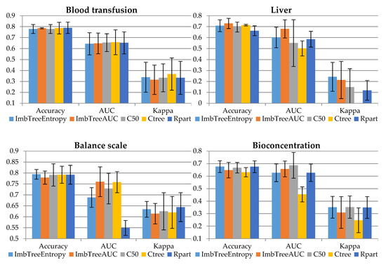
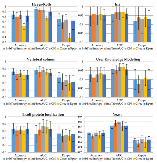
Figure 1.
Comparison of classification accuracy results.
Table 3.
Comparison of tree structures in terms of number of leaves and predicted classes.
In the following section, the results will be discussed using the validation sample. Detailed results for validation sample are provided in Appendix A (Table A1).
The results obtained by ImbTreeEntropy and ImbTreeAUC for Blood transfusion data set are of similar accuracy to those observed for the C50, Ctree or Rpart algorithms. All the algorithms were able to discover 2 classes, by producing non-complex trees, i.e., having between 4 and 7 leaves.
Based on the binary Liver data set, the results of ImbTreeEntropy and ImbTreeAUC are considerably better than those observed for the C50, Ctree or Rpart benchmarks. Both algorithms have identified proper number of classes in the data set, with relatively simple tree structures having 7.2 and 11.7 leaves, on average, for ImbTreeEntropy and ImbTreeAUC, respectively.
Balance scale is a three-class problem and ImbTreeAUC algorithm was able to predict it to a great extent. ImbTreeEntropy was outperformed by C50, Ctree, taking into account AUC, however, Ctree could recognize 2.6 classes, on average, out of 3.
The bioconcentration data set is another three-class problem and the accuracy of both proposed algorithms are in the forefront when it comes to the AUC and Kappa. Although AUC for C50 is the highest, the algorithm produced very complex tree with 52.6 leaves, on average, which is considered a significant drawback.
The Hayes–Roth data set is relatively easy for classification as all the algorithms, except Ctree, delivered good classification accuracy with AUC more than 0.90. In particular, AUC for ImbTreeEntropy was the highest: 0.953. The results for balanced Iris data set show that both algorithms, i.e., ImbTreeAUC and ImbTreeEntropy, have similar performance to the results delivered by other packages, in in terms of AUC, accuracy, and Kappa. Importantly, all the algorithms were able to discover 3 classes.
Finally, the Vertebral column data set was the last example with three classes. It was ImbTreeEntropy which outperformed the other algorithms, in terms of AUC and Kappa, and additionally, the tree structure was simple with 5.5 leaves only, on average.
The User knowledge modelling dataset, which is four class problem, is relatively easy for classification. The results, in in terms of AUC, accuracy and Kappa, for both algorithms are very similar to the performance of benchmarking algorithms. Once again, ImbTreeAUC provides the tree with simpler structure, i.e., with 7 leaves only, on average, while other trees are more complex. As previously for a 3-class problem, all the algorithms were able to discover 4 classes.
The following data set, which is E. coli protein localization sites, is highly imbalanced, with huge underrepresentation of three classes out of eight. The results indicate that ImbTreeEntropy and ImbTreeAUC algorithms are able to outperform other methods, due to the fact that they could identify all 8 classes in the dataset, keeping good accuracy, AUC and Kappa at the same time. The benchmark algorithms could identify 6, 6.7 or 5.7 classes, on average, only.
Finally, the Yeast data set describes a 10 class problem and it is very imbalanced, with huge underrepresentation of six classes out of 10. The results indicate that C50 outperformed other methods, in terms of AUC and Kappa, however, the tree is very complex, with 93.4 leaves, on average. ImbTreeEntropy and ImbTreeAUC algorithms provide slightly worse results, but these could identify nearly 10 classes in the dataset, while keeping good AUC and Kappa at the same time. Ctree and Rpart algorithms could identify 8 and 7.9 classes (out of 10), on average, only.
Based on the experiments we conclude that both packages offer accurate classification in case of imbalanced data sets, with the ability to recognize a proper number of classes, often using less complex trees.
Additionally, the Table A2 from the Appendix A consist of the results obtained based on the state-of-the-art algorithms. The K-nearest neighbor (KNN) algorithm has been implemented using knn3 function from the caret package while the artificial neural network (NNET) algorithm has been implemented based on the nnet library. Both algorithms have been properly tuned i.e., in KNN there was only one tuned parameter k, while in NNET there were three tuned parameters, number of hidden neurons, weights decay and number of iterations.
5. Conclusions
Decision trees are popular methods used by academics and by business. Their attractiveness is due to the fact that trees create rules that are easily interpretable and easy implementable in business practice. Although decision trees have numerous benefits, they tend to deliver lower predictive accuracy in the case of imbalanced data. We believe our novel software packages, ImbTreeEntropy and ImbTreeAUC, applicable to binary and multi-class problems, address that gap. No data pre-processing is required as the packages accept all types of attributes, including continuous, ordered and nominal.
Importantly, ImbTreeEntropy implements a couple of generalized entropies as impurity measures which makes it more attractive than standard tree algorithms based on Shannon entropy or Gini index as these do not allow for exploration of the trade-off between the probability of different classes and the overall information gain. As far as ImbTreeAUC is concerned, it applies AUC as impurity measure which an appealing concept implemented in decision tree algorithm.
Based on the experiments conducted on 10 freely available data sets we conclude that our packages can be particularly useful for datasets with one or more minority classes. In particular, both algorithms proposed by the authors deliver the performance of similar quality in comparison to the benchmark algorithms; however, the trees created by ImbTreeEntropy and ImbTreeAUC are often less complex which is considered a significant advantage. Importantly, both algorithms are able to outperform other methods as both are able to identify multiple classes correctly, especially in cases when a large number of classes is to be predicted.
We intend to further enhance the packages so these can visualize the tree as a rule-based model. Additionally, an interactive learning process would be proposed so the expert can make a decision regarding the optimal split in ambiguous situations.
Author Contributions
Funding
This research received no external funding.
Conflicts of Interest
The authors declare no conflict of interest.
Appendix A. Comparison of Classification Results
The results from the folds were averaged to produce the measures with standard deviation provided in brackets. The accuracy measures include sensitivity, specificity, positive predictive value, negative predictive value, prevalence and detection rate. For some data sets, the value of the measure is not provided (NA) because there were no observations for some classes in the validation folds.
Table A1.
Additional performance measures.
Table A1.
Additional performance measures.
| Algorithm | Sensitivity | Specificity | Pos Pred Value | Neg Pred Value | Prevalence | Detection Rate |
|---|---|---|---|---|---|---|
| Blood transfusion data | ||||||
| ImbTreeEntropy | 0.886 (∓0.039) | 0.432 (∓0.137) | 0.835 (∓0.034) | 0.541 (∓0.115) | 0.762 (∓0.004) | 0.675 (∓0.03) |
| ImbTreeAUC | 0.921 (∓0.057) | 0.348 (∓0.09) | 0.819 (∓0.023) | 0.616 (∓0.188) | 0.762 (∓0.004) | 0.702 (∓0.042) |
| C50 | 0.891 (∓0.057) | 0.449 (∓0.119) | 0.839 (∓0.032) | 0.581 (∓0.165) | 0.762 (∓0.004) | 0.679 (∓0.042) |
| Ctree | 0.889 (∓0.047) | 0.422 (∓0.137) | 0.832 (∓0.032) | 0.553 (∓0.112) | 0.762 (∓0.004) | 0.678 (∓0.035) |
| Rpart | 0.919 (∓0.055) | 0.371 (∓0.116) | 0.824 (∓0.029) | 0.616 (∓0.178) | 0.762 (∓0.004) | 0.701 (∓0.041) |
| Liver data | ||||||
| ImbTreeEntropy | 0.909 (∓0.058) | 0.281 (∓0.179) | 0.762 (∓0.044) | 0.552 (∓0.266) | 0.714 (∓0.007) | 0.648 (∓0.04) |
| ImbTreeAUC | 0.834 (∓0.077) | 0.395 (∓0.133) | 0.776 (∓0.034) | 0.511 (∓0.124) | 0.714 (∓0.007) | 0.595 (∓0.054) |
| C50 | 1 (∓0) | 0 (∓0) | 0.714 (∓0.007) | NA (∓NA) | 0.714 (∓0.007) | 0.714 (∓0.007) |
| Ctree | 0.861 (∓0.103) | 0.287 (∓0.242) | 0.756 (∓0.052) | NA (∓NA) | 0.714 (∓0.007) | 0.614 (∓0.073) |
| Rpart | 0.802 (∓0.092) | 0.311 (∓0.134) | 0.745 (∓0.025) | 0.384 (∓0.081) | 0.714 (∓0.007) | 0.573 (∓0.068) |
| Balance scale data | ||||||
| ImbTreeEntropy | 0.579 (∓0.023) | 0.888 (∓0.011) | 0.572 (∓0.024) | 0.893 (∓0.014) | 0.333 (∓0) | 0.265 (∓0.007) |
| ImbTreeAUC | 0.586 (∓0.036) | 0.884 (∓0.014) | 0.588 (∓0.043) | 0.885 (∓0.018) | 0.333 (∓0) | 0.26 (∓0.01) |
| C50 | 0.578 (∓0.033) | 0.876 (∓0.026) | NA (∓NA) | 0.89 (∓0.026) | 0.333 (∓0) | 0.264 (∓0.013) |
| Ctree | 0.572 (∓0.036) | 0.883 (∓0.027) | NA (∓NA) | 0.89 (∓0.03) | 0.333 (∓0) | 0.264 (∓0.017) |
| Rpart | 0.578 (∓0.036) | 0.9 (∓0.017) | 0.599 (∓0.017) | 0.894 (∓0.025) | 0.333 (∓0) | 0.264 (∓0.014) |
| Bioconcentration data | ||||||
| ImbTreeEntropy | 0.514 (∓0.042) | 0.778 (∓0.029) | 0.69 (∓0.128) | 0.799 (∓0.037) | 0.333 (∓0) | 0.225 (∓0.016) |
| ImbTreeAUC | 0.513 (∓0.056) | 0.766 (∓0.044) | 0.567 (∓0.106) | 0.778 (∓0.046) | 0.333 (∓0) | 0.216 (∓0.021) |
| C50 | 0.432 (∓0.041) | 0.747 (∓0.035) | NA (∓NA) | 0.758 (∓0.034) | 0.333 (∓0) | 0.21 (∓0.012) |
| Ctree | 0.553 (∓0.08) | 0.78 (∓0.032) | 0.645 (∓0.098) | 0.79 (∓0.032) | 0.333 (∓0) | 0.222 (∓0.014) |
| Rpart | 0.514 (∓0.043) | 0.778 (∓0.029) | 0.689 (∓0.128) | 0.798 (∓0.037) | 0.333 (∓0) | 0.225 (∓0.016) |
| Hayes–Roth data | ||||||
| ImbTreeEntropy | 0.871 (∓0.062) | 0.913 (∓0.042) | 0.881 (∓0.055) | 0.918 (∓0.038) | 0.333 (∓0) | 0.281 (∓0.025) |
| ImbTreeAUC | 0.822 (∓0.087) | 0.892 (∓0.046) | 0.85 (∓0.064) | 0.899 (∓0.043) | 0.333 (∓0) | 0.268 (∓0.028) |
| C50 | 0.677 (∓0.04) | 0.782 (∓0.032) | NA (∓NA) | 0.842 (∓0.045) | 0.333 (∓0) | 0.204 (∓0.019) |
| Ctree | 0.856 (∓0.055) | 0.903 (∓0.039) | 0.873 (∓0.044) | 0.911 (∓0.031) | 0.333 (∓0) | 0.275 (∓0.024) |
| Rpart | 0.856 (∓0.089) | 0.902 (∓0.061) | NA (∓NA) | 0.928 (∓0.036) | 0.333 (∓0) | 0.274 (∓0.037) |
| Iris data | ||||||
| ImbTreeEntropy | 0.947 (∓0.053) | 0.973 (∓0.026) | 0.955 (∓0.046) | 0.976 (∓0.024) | 0.333 (∓0) | 0.316 (∓0.018) |
| ImbTreeAUC | 0.96 (∓0.047) | 0.98 (∓0.023) | 0.968 (∓0.035) | 0.982 (∓0.02) | 0.333 (∓0) | 0.32 (∓0.016) |
| C50 | 0.96 (∓0.034) | 0.98 (∓0.017) | 0.967 (∓0.029) | 0.982 (∓0.016) | 0.333 (∓0) | 0.32 (∓0.011) |
| Ctree | 0.953 (∓0.055) | 0.977 (∓0.027) | 0.96 (∓0.048) | 0.978 (∓0.026) | 0.333 (∓0) | 0.318 (∓0.018) |
| Rpart | 0.953 (∓0.032) | 0.977 (∓0.016) | 0.961 (∓0.027) | 0.979 (∓0.015) | 0.333 (∓0) | 0.318 (∓0.011) |
| Vertebral column data | ||||||
| ImbTreeEntropy | 0.789 (∓0.061) | 0.921 (∓0.023) | 0.8 (∓0.056) | 0.922 (∓0.025) | 0.333 (∓0) | 0.277 (∓0.017) |
| ImbTreeAUC | 0.77 (∓0.096) | 0.917 (∓0.033) | 0.789 (∓0.1) | 0.919 (∓0.036) | 0.333 (∓0) | 0.274 (∓0.024) |
| C50 | 0.779 (∓0.082) | 0.91 (∓0.039) | 0.79 (∓0.069) | 0.916 (∓0.03) | 0.333 (∓0) | 0.271 (∓0.022) |
| Ctree | 0.798 (∓0.054) | 0.924 (∓0.022) | 0.807 (∓0.063) | 0.926 (∓0.022) | 0.333 (∓0) | 0.278 (∓0.015) |
| Rpart | 0.786 (∓0.072) | 0.916 (∓0.029) | 0.785 (∓0.077) | 0.915 (∓0.03) | 0.333 (∓0) | 0.272 (∓0.021) |
| User knowledge modeling data | ||||||
| ImbTreeEntropy | 0.849 (∓0.099) | 0.956 (∓0.023) | NA (∓NA) | 0.963 (∓0.017) | 0.25 (∓0) | 0.22 (∓0.016) |
| ImbTreeAUC | 0.9 (∓0.036) | 0.968 (∓0.013) | 0.932 (∓0.032) | 0.971 (∓0.012) | 0.25 (∓0) | 0.228 (∓0.009) |
| C50 | 0.92 (∓0.039) | 0.977 (∓0.011) | 0.953 (∓0.024) | 0.979 (∓0.01) | 0.25 (∓0) | 0.234 (∓0.008) |
| Ctree | 0.923 (∓0.045) | 0.975 (∓0.013) | 0.934 (∓0.045) | 0.976 (∓0.014) | 0.25 (∓0) | 0.232 (∓0.01) |
| Rpart | 0.917 (∓0.048) | 0.974 (∓0.015) | 0.943 (∓0.034) | 0.976 (∓0.014) | 0.25 (∓0) | 0.232 (∓0.01) |
| E. coli protein localization data | ||||||
| ImbTreeEntropy | NA (∓NA) | 0.965 (∓0.01) | NA (∓NA) | NA (∓NA) | 0.125 (∓0) | 0.097 (∓0.008) |
| ImbTreeAUC | NA (∓NA) | 0.967 (∓0.008) | NA (∓NA) | NA (∓NA) | 0.125 (∓0) | 0.099 (∓0.008) |
| C50 | NA (∓NA) | 0.97 (∓0.01) | NA (∓NA) | NA (∓NA) | 0.125 (∓0) | 0.101 (∓0.007) |
| Ctree | NA (∓NA) | 0.97 (∓0.009) | NA (∓NA) | NA (∓NA) | 0.125 (∓0) | 0.102 (∓0.007) |
| Rpart | NA (∓NA) | 0.971 (∓0.015) | NA (∓NA) | NA (∓NA) | 0.125 (∓0) | 0.105 (∓0.01) |
| Yeast data | ||||||
| ImbTreeEntropy | NA (∓NA) | 0.943 (∓0.005) | NA (∓NA) | NA (∓NA) | 0.1 (∓0) | 0.058 (∓0.004) |
| ImbTreeAUC | NA (∓NA) | 0.935 (∓0.005) | NA (∓NA) | NA (∓NA) | 0.1 (∓0) | 0.051 (∓0.005) |
| C50 | NA (∓NA) | 0.938 (∓0.011) | NA (∓NA) | NA (∓NA) | 0.1 (∓0) | 0.055 (∓0.007) |
| Ctree | NA (∓NA) | 0.945 (∓0.007) | NA (∓NA) | NA (∓NA) | 0.1 (∓0) | 0.059 (∓0.005) |
| Rpart | NA (∓NA) | 0.943 (∓0.006) | NA (∓NA) | NA (∓NA) | 0.1 (∓0) | 0.058 (∓0.005) |
Table A2.
Results of the state-of-the-art algorithms.
Table A2.
Results of the state-of-the-art algorithms.
| Dataset | KNN | NNET | ||||
|---|---|---|---|---|---|---|
| Accuracy | AUC | Kappa | Accuracy | AUC | Kappa | |
| Blood transfusion data | 0.795 (∓0.037) | 0.746 (∓0.061) | 0.320 (∓0.120) | 0.806 (∓0.035) | 0.767 (∓0.062) | 0.357 (∓0.135) |
| Liver data | 0.649 (∓0.072) | 0.465 (∓0.094) | 0.183 (∓0.132) | 0.727 (∓0.054) | 0.273 (∓0.066) | 0.276 (∓0.168) |
| Balance scale data | 0.902 (∓0.011) | 0.877 (∓0.065) | 0.819 (∓0.022) | 0.978 (∓0.010) | 0.997 (∓0.002) | 0.961 (∓0.017) |
| Bioconcentration data | 0.649 (∓0.049) | 0.599 (∓0.087) | 0.312 (∓0.103) | 0.685 (∓0.047) | 0.738 (∓0.071) | 0.374 (∓0.0109) |
| Hayes–Roth data | 0.698 (∓0.087) | 0.777 (∓0.092) | 0.51 (∓0.148) | 0.806 (∓0.116) | 0.955 (∓0.065) | 0.694 (∓0.183) |
| Iris data | 0.967 (∓0.035) | 0.999 (∓0.003) | 0.950 (∓0.053) | 0.973 (∓0.034) | 0.997 (∓0.006) | 0.960 (∓0.052) |
| Vertebral column data | 0.794 (∓0.065) | 0.896 (∓0.043) | 0.668 (∓0.104) | 0.871 (∓0.070) | 0.949 (∓0.035) | 0.793 (∓0.112) |
| User knowledge modeling data | 0.878 (∓0.067) | 0.956 (∓031) | 0.831 (∓0.094) | 0.960 (∓0.029) | 0.995 (∓0.006) | 0.945 (∓0.040) |
| E. coli protein localization data | 0.872 (∓0.040) | 0.908 (∓0.078) | 0.823 (∓0.054) | 0.887 (∓0.026) | 0.950 (∓0.040) | 0.843 (∓0.034) |
| Yeast data | 0.597 (∓0.049) | 0.826 (∓0.050) | 0.472 (∓0.064) | 0.613 (∓0.033) | 0.856 (∓0.040) | 0.495 (∓0.041) |
References
- Rout, N.; Mishra, D.; Mallick, M.K. Handling Imbalanced Data: A Survey. Int. Proc. Adv. Soft Comput. Intell. Syst. Appl. 2017, 431–443. [Google Scholar] [CrossRef]
- Wang, S.; Yao, X. Multiclass Imbalance Problems: Analysis and Potential Solutions. IEEE Trans. Syst. Mancybern. Part B (Cybern.) 2012, 42, 1119–1130. [Google Scholar] [CrossRef]
- Lakshmi, T.J.; Prasad, C.S.R. A study on classifying imbalanced datasets. In Proceedings of the First International Conference on Networks & Soft Computing (ICNSC2014), Guntur, India, 19–20 August 2014. [Google Scholar] [CrossRef]
- Leevy, J.L.; Khoshgoftaar, T.M.; Bauder, R.A.; Seliya, N. A survey on addressing high-class imbalance in big data. J. Big Data 2018, 5. [Google Scholar] [CrossRef]
- Quinlan, J.R. Induction of decision trees. Mach. Learn. 1986, 1, 81–106. [Google Scholar] [CrossRef]
- Breiman, L.; Friedman, J.H.; Olshen, R.A.; Stone, C.J. Classification and Regression Trees; Wadsworth Statistics/Probability Series; CRC Press: Boca Raton, FL, USA, 1984. [Google Scholar] [CrossRef]
- Kass, G.V. An Exploratory Technique for Investigating Large Quantities of Categorical Data. Appl. Stat. 1980, 29, 119. [Google Scholar] [CrossRef]
- Available online: https://archive.ics.uci.edu/ml/index.php (accessed on 10 October 2020).
- Galar, M.; Fernandez, A.; Barrenechea, E.; Bustince, H.; Herrera, F. A Review on Ensembles for the Class Imbalance Problem: Bagging-, Boosting-, and Hybrid-Based Approaches. IEEE Trans. Syst. Mancybern. Part C (Appl. Rev.) 2012, 42, 463–484. [Google Scholar] [CrossRef]
- Pérez-Godoy, M.D.; Rivera, A.J.; Carmona, C.J.; del Jesus, M.J. Training algorithms for Radial Basis Function Networks to tackle learning processes with imbalanced data-sets. Appl. Soft Comput. 2014, 25, 26–39. [Google Scholar] [CrossRef]
- Sáez, J.A.; Luengo, J.; Stefanowski, J.; Herrera, F. SMOTE–IPF: Addressing the noisy and borderline examples problem in imbalanced classification by a re-sampling method with filtering. Inf. Sci. 2015, 291, 184–203. [Google Scholar] [CrossRef]
- Błaszczyński, J.; Stefanowski, J. Neighbourhood sampling in bagging for imbalanced data. Neurocomputing 2015, 150, 529–542. [Google Scholar] [CrossRef]
- Majid, A.; Ali, S.; Iqbal, M.; Kausar, N. Prediction of human breast and colon cancers from imbalanced data using nearest neighbor and support vector machines. Comput. Methods Programs Biomed. 2014, 113, 792–808. [Google Scholar] [CrossRef] [PubMed]
- Maratea, A.; Petrosino, A.; Manzo, M. Adjusted F-measure and kernel scaling for imbalanced data learning. Inf. Sci. 2014, 257, 331–341. [Google Scholar] [CrossRef]
- Maldonado, S.; López, J. Imbalanced data classification using second-order cone programming support vector machines. Pattern Recognit. 2014, 47, 2070–2079. [Google Scholar] [CrossRef]
- Datta, S.; Das, S. Near-Bayesian Support Vector Machines for imbalanced data classification with equal or unequal misclassification costs. Neural Netw. 2015, 70, 39–52. [Google Scholar] [CrossRef] [PubMed]
- Alibeigi, M.; Hashemi, S.; Hamzeh, A. DBFS: An effective Density Based Feature Selection scheme for small sample size and high dimensional imbalanced data sets. Data Knowl. Eng. 2012, 81–82, 67–103. [Google Scholar] [CrossRef]
- Domingos, P. MetaCost. In Proceedings of the Fifth ACM SIGKDD International Conference on Knowledge Discovery and Data Mining—KDD ‘99, San Diego, CA, USA, 12–18 August 1999. [Google Scholar] [CrossRef]
- Thai-Nghe, N.; Gantner, Z.; Schmidt-Thieme, L. Cost-sensitive learning methods for imbalanced data. In Proceedings of the 2010 International Joint Conference on Neural Networks (IJCNN), Barcelona, Spain, 18–23 July 2010. [Google Scholar] [CrossRef]
- Gajowniczek, K.; Ząbkowski, T.; Sodenkamp, M. Revealing Household Characteristics from Electricity Meter Data with Grade Analysis and Machine Learning Algorithms. Appl. Sci. 2018, 8, 1654. [Google Scholar] [CrossRef]
- Gajowniczek, K.; Nafkha, R.; Ząbkowski, T. Electricity peak demand classification with artificial neural networks. In Proceedings of the 2017 Federated Conference on Computer Science and Information Systems, Prague, Czech Republic, 3–6 September 2017. [Google Scholar] [CrossRef]
- Gajowniczek, K.; Orłowski, A.; Ząbkowski, T. Entropy Based Trees to Support Decision Making for Customer Churn Management. Acta Phys. Pol. A 2016, 129, 971–979. [Google Scholar] [CrossRef]
- Elkan, C. The foundations of cost-sensitive learning. In Proceedings of the International Joint Conference on Artificial Intelligence, Seattle, WA, USA, 4–10 August 2001; Lawrence Erlbaum Associates Ltd.: Mahwah, NJ, USA, 2001; Volume 17, pp. 973–978. [Google Scholar]
- Zadrozny, B.; Langford, J.; Abe, N. Cost-sensitive learning by cost-proportionate example weighting. In Proceedings of the Third IEEE International Conference on Data Mining, Melbourne, FL, USA, 19–22 November 2003. [Google Scholar] [CrossRef]
- Buntine, W. Learning classification trees. Artif. Intell. Front. Stat. 1993, 182–201. [Google Scholar] [CrossRef]
- Taylor, P.C.; Silverman, B.W. Block diagrams and splitting criteria for classification trees. Stat. Comput. 1993, 3, 147–161. [Google Scholar] [CrossRef]
- Mola, F.; Siciliano, R. A fast splitting procedure for classification trees. Stat. Comput. 1997, 7, 209–216. [Google Scholar] [CrossRef]
- Kearns, M.; Mansour, Y. On the Boosting Ability of Top–Down Decision Tree Learning Algorithms. J. Comput. Syst. Sci. 1999, 58, 109–128. [Google Scholar] [CrossRef]
- Rokach, L.; Maimon, O. Decision trees. In Data Mining and Knowledge Discovery Handbook; Springer: Boston, MA, USA, 2005; pp. 165–192. [Google Scholar]
- Fayyad, U.M.; Irani, K.B. The Attribute Selection Problem in Decision Tree Generation; AAAI Press: Palo Alto, CA, USA, 1992; pp. 104–110. [Google Scholar]
- Rounds, E.M. A combined nonparametric approach to feature selection and binary decision tree design. Pattern Recognit. 1980, 12, 313–317. [Google Scholar] [CrossRef]
- Ferri, C.; Flach, P.; Hernández-Orallo, J. Learning decision trees using the area under the ROC curve. In Conference: Machine Learning. In Proceedings of the Nineteenth International Conference (ICML 2002), University of New South Wales, Sydney, Australia, 8–12 July 2002. [Google Scholar]
- Gajowniczek, K.; Liang, Y.; Friedman, T.; Ząbkowski, T.; Van den Broeck, G. Semantic and Generalized Entropy Loss Functions for Semi-Supervised Deep Learning. Entropy 2020, 22, 334. [Google Scholar] [CrossRef]
- Nafkha, R.; Gajowniczek, K.; Ząbkowski, T. Do Customers Choose Proper Tariff? Empirical Analysis Based on Polish Data Using Unsupervised Techniques. Energies 2018, 11, 514. [Google Scholar] [CrossRef]
- Sharma, B.D.; Mittal, B.D. Development of a pressure chemical doser. J. Inst. Eng. Public Health Eng. Div. 1975, 56, 28–32. [Google Scholar]
- Masi, M. A step beyond Tsallis and Rényi entropies. Phys. Lett. A 2005, 338, 217–224. [Google Scholar] [CrossRef]
- Sharma, B.D.; Taneja, I.J. Entropy of type (α, β) and other generalized measures in information theory. Metrika 1975, 22, 205–215. [Google Scholar] [CrossRef]
- Kapur, J.N. Some Properties of Entropy of Order α and Type β; Springer: New Delhi, India, 1969; Volume 69, No. 4; pp. 201–211. [Google Scholar]
- Mann, H.B.; Whitney, D.R. On a Test of Whether one of Two Random Variables is Stochastically Larger than the Other. Ann. Math. Stat. 1947, 18, 50–60. [Google Scholar] [CrossRef]
- Hand, D.J.; Till, R.J. A Simple Generalisation of the Area Under the ROC Curve for Multiple Class Classification Problems. Mach. Learn. 2001, 45, 171–186. [Google Scholar] [CrossRef]
- O’Brien, D.B.; Gupta, M.R.; Gray, R.M. Cost-sensitive multi-class classification from probability estimates. In Proceedings of the 25th International Conference on Machine Learning—ICML, Helsinki, Finland, 5–9 July 2008. [Google Scholar] [CrossRef]
- Ling, C.X.; Sheng, V.S. Cost-Sensitive Learning. Encycl. Mach. Learn. Data Min. 2017, 285–289. [Google Scholar] [CrossRef]
- Xiang, Y.; Gubian, S.; Suomela, B.; Hoeng, J. Generalized Simulated Annealing for Global Optimization: The GenSA Package. R. J. 2013, 5, 13. [Google Scholar] [CrossRef]
- Wright, M.N.; König, I.R. Splitting on categorical predictors in random forests. PeerJ 2019, 7, e6339. [Google Scholar] [CrossRef] [PubMed]
- Fisher, W.D. On Grouping for Maximum Homogeneity. J. Am. Stat. Assoc. 1958, 53, 789–798. [Google Scholar] [CrossRef]
- Mehta, M.; Agrawal, R.; Rissanen, J. SLIQ: A fast scalable classifier for data mining. Lect. Notes Comput. Sci. 1996, 18–32. [Google Scholar] [CrossRef]
- Gnanadesikan, R. Methods for Statistical Data Analysis of Multivariate Observations; John Wiley & Sons: New York, NY, USA, 2011; Volume 321. [Google Scholar]
- Coppersmith, D.; Hong, S.J.; Hosking, J.R. Partitioning nominal attributes in decision trees. Data Min. Knowl. Discov. 1999, 3, 197–217. [Google Scholar] [CrossRef]
- Yeh, I.C.; Yang, K.J.; Ting, T.M. Knowledge discovery on RFM model using Bernoulli sequence. Expert Syst. Appl. 2009, 36, 5866–5871. [Google Scholar] [CrossRef]
- Ramana, B.V.; Babu, M.S.P.; Venkateswarlu, N.B. A critical comparative study of liver patients from USA and INDIA: An exploratory analysis. Int. J. Comput. Sci. Issues 2012, 9, 506–516. [Google Scholar]
- Klahr, D.; Siegler, R.S. The representation of children’s knowledge. Adv. Child Dev. Behav. 1978, 12, 61–116. [Google Scholar]
- Grisoni, F.; Consonni, V.; Vighi, M.; Villa, S.; Todeschini, R. Investigating the mechanisms of bioconcentration through QSAR classification trees. Env. Int. 2016, 88, 198–205. [Google Scholar] [CrossRef]
- Hayes-Roth, B.; Hayes-Roth, F. Concept learning and the recognition and classification of exemplars. J. Verbal Learn. Verbal Behav. 1977, 16, 321–338. [Google Scholar] [CrossRef]
- Duda, R.O.; Hart, P.E.; Stork, D.G. Pattern Classification. J. Classif. 2001, 24, 305–307. [Google Scholar] [CrossRef]
- Rocha Neto, A.R.; Alencar Barreto, G. On the application of ensembles of classifiers to the diagnosis of pathologies of the vertebral column: A comparative analysis. IEEE Lat. Am. Trans. 2009, 7, 487–496. [Google Scholar] [CrossRef]
- Kahraman, H.T.; Sagiroglu, S.; Colak, I. The development of intuitive knowledge classifier and the modeling of domain dependent data. Knowl. Based Syst. 2013, 37, 283–295. [Google Scholar] [CrossRef]
- Horton, P.; Nakai, K. A probabilistic classification system for predicting the cellular localization sites of proteins. ISMB 1996, 4, 109–115. [Google Scholar] [PubMed]
- Nakai, K.; Kanehisa, M. A knowledge base for predicting protein localization sites in eukaryotic cells. Genomics 1992, 14, 897–911. [Google Scholar] [CrossRef]
- Fawcett, T. Introduction to ROC analysis. Pattern Recognit. Lett. 2008, 27, 861–874. [Google Scholar] [CrossRef]
- Cohen, J. A Coefficient of Agreement for Nominal Scales. Educ. Psychol. Meas. 1960, 20, 37–46. [Google Scholar] [CrossRef]
Publisher’s Note: MDPI stays neutral with regard to jurisdictional claims in published maps and institutional affiliations. |
© 2021 by the authors. Licensee MDPI, Basel, Switzerland. This article is an open access article distributed under the terms and conditions of the Creative Commons Attribution (CC BY) license (http://creativecommons.org/licenses/by/4.0/).