Article

Rescheduling of Distributed Manufacturing System with Machine Breakdowns

1
School of Electrical and Control Engineering, Xuzhou University of Technology, Xuzhou 221018, China
2
School of Computer Science, Liaocheng University, Liaocheng 252000, China
3
Department of Manufacturing Engineering and Automation Products, Opole University of Technology, 45-758 Opole, Poland
4
Department of Electrical, Control and Computer Engineering, Opole University of Technology, 45-758 Opole, Poland
*
Author to whom correspondence should be addressed.
Electronics 2022, 11(2), 249; https://doi.org/10.3390/electronics11020249
Submission received: 5 December 2021 / Revised: 8 January 2022 / Accepted: 10 January 2022 / Published: 13 January 2022

Abstract

:
This study attempts to explore the dynamic scheduling problem from the perspective of operational research optimization. The goal is to propose a rescheduling framework for solving distributed manufacturing systems that consider random machine breakdowns as the production disruption. We establish a mathematical model that can better describe the scheduling of the distributed blocking flowshop. To realize the dynamic scheduling, we adopt an “event-driven” policy and propose a two-stage “predictive-reactive” method consisting of two steps: initial solution pre-generation and rescheduling. In the first stage, a global initial schedule is generated and considers only the deterministic problem, i.e., optimizing the maximum completion time of static distributed blocking flowshop scheduling problems. In the second stage, that is, after the breakdown occurs, the rescheduling mechanism is triggered to seek a new schedule so that both maximum completion time and the stability measure of the system can be optimized. At the breakdown node, the operations of each job are classified and a hybrid rescheduling strategy consisting of “right-shift repair + local reorder” is performed. For local reorder, we designed a discrete memetic algorithm, which embeds the differential evolution concept in its search framework. To test the effectiveness of DMA, comparisons with mainstream algorithms are conducted on instances with different scales. The statistical results show that the ARPDs obtained from DMA are improved by 88%.

1. Introduction

With the advancement of economic globalization and the intensification of mergers between enterprises, the emergence of large-scale or concurrent production makes the pattern of distributed manufacturing necessary [1,2]. Distributed manufacturing decentralizes tasks into factories or workshops from different geographical locations. This pattern can help the manufacturers raise productivity, reduce cost, control risks, and adjust marketing policies more flexibly [3]. As an important part of distributed manufacturing, scheduling directly affects the efficiency and competitiveness of enterprises. Generally speaking, to solve such problems, a problem-specific model with production constraints should be first established to describe the scheduling problem considered. Then, optimization methods (e.g., mathematical programming, intelligent optimization, etc.) of operational research are developed to search for an optimal solution. For systems with large-scale and high complexity, mathematical programming such as integer programming, branch and bound, dynamic programming, or cut plane can rarely find an optimal solution (ranking) in the target space due to enumeration concept, but the efficiency decreases with the increment of the number of jobs/tasks to be scheduled.
At present, most studies use intelligent optimization algorithms to approximate the optimal solution for scheduling problems. The intelligent optimization algorithm, also called the evolutionary optimization algorithm, or metaheuristic, reveals the design principle of optimization algorithm through the understanding of relevant behavior, function, rules, and action mechanism in biological, physical, chemical, social, artistic, and other systems or fields. It refines the corresponding feature model under the guidance of the characteristics of specific problems and designs an intelligent iterative search process. That is, these kinds of algorithms do not rely on the characteristics of problems, but obtain near-optimal solutions through continuous iterations of global and local search. When an intelligent algorithm is applied for scheduling problems, it can express the schedule as a permutation model in the form of coding, and further compress the solution space into a very flat space, so that a large number of different permutations (schedules) correspond to the same target. Hence, the permutation model-based algorithm can search more different schedules in the target space range in tens of milliseconds to tens of seconds, so as to obtain a solution better than the traditional mathematical programming method.
The object of this study is related to the distributed blocking flowshop scheduling problem (DBFSP) [4]. 
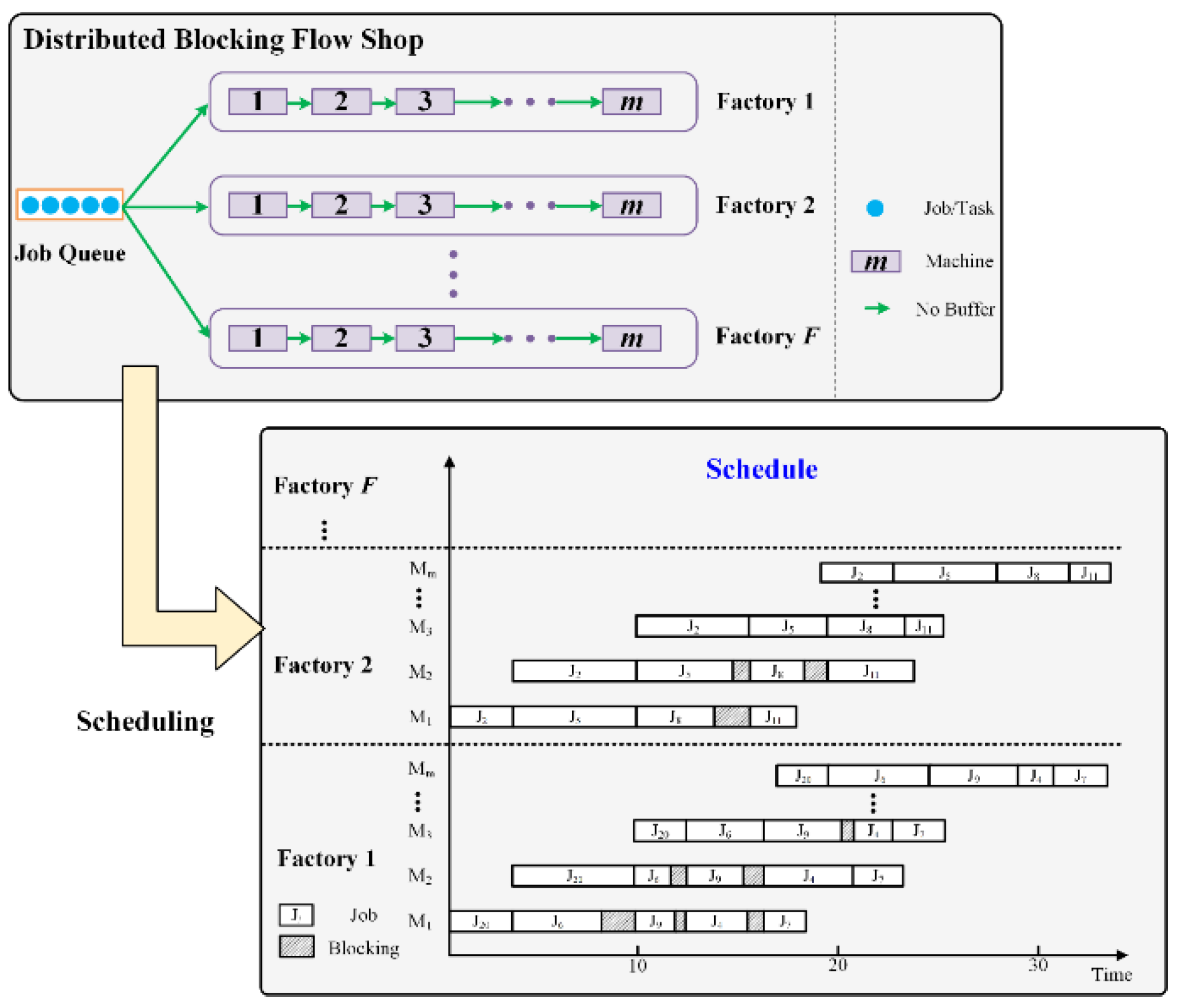
Figure 1 illustrates DBFSP, which considers f parallel factories that contain the same machine configurations and technological processes [5]. The jobs can be assigned to any factories and each job follows the same blocking manufacturing procedure [6]. Although the machines configured in each distributed factory are the same, the processing time of each operation of each job is assumed to be different, thereby the processing tasks assigned to each distributed factory and their completion time are also different. The idea of solving DBFSP is to reasonably allocate the jobs to the factory through optimization algorithms, and then sequence the jobs in each distributed factory, to optimize the manufacturing objectives of the whole work order. Currently, researchers have made great efforts on solving DBFSP in a static environment, the existing researches mainly focused on the construction of mathematical models and the design of optimization algorithms. Zhang et al. [7] have established two different mathematical models using forward and reverse recursion approaches. A hybrid discrete differential evolution (DDE) algorithm was proposed to minimize the maximum completion time (makespan). Zhang et al. [8] constructed the mixed-integer model for DBFSP and developed a discrete fruit fly algorithm (DFOA) with a speed-up mechanism to minimize the global makespan. Additionally, Shao et al. [9] proposed a hybrid enhanced discrete fruit fly optimization algorithm (HEDFOA) to optimize the makespan. A new assignment rule and an insertion-based improvement procedure were developed to initialize the common central location of different fruit fly swarms. Li et al. [10] investigated a special case of DBFSP, in which a transport robot was embedded in each factory. The loading and unloading times are considered and different for all of the jobs conducted by the robot. An improved iterated greedy (IIG) algorithm was proposed to improve productivity. Moreover, Zhao et al. [11] proposed an ensemble discrete differential evolution (EDE) algorithm, in which three initialization heuristics that consider the front delay, blocking time, and idle time were designed. The mutation, crossover, and selection operators are redesigned to assist the EDE algorithm to execute in the discrete domain.
The above researches on DBFSP have formed a certain system, but they assumed that no explicit disruptions occur during the manufacturing process. In fact, a series of uncertainties often happened during the manufacturing process [12]. These uncertainties, which are sudden and uncontrollable, can change the state of the system strongly and affect the scheduling activities continuously [13]. As a result, the original static schedules are no longer suitable for real-time scheduling. To eliminate the impact of sudden uncertainties, rescheduling operations are generally performed in response to disruptions [14,15]. Rescheduling refers to the procedure of modifying the existing schedule to obtain a new feasible one after uncertain events occur [16]. One of the most important rescheduling strategies for traditional flowshop is “predictive-reactive” scheduling [17]. “predictive-reactive” scheduling defines a two-stage “event-driven” scheduling operation: the first stage generates an initial schedule that provides a baseline reference for other manufactural activities such as procurement and distribution of raw materials [18]. Influenced by the disruptions, the second stage explicitly quantifies the disruptions, constructs the management model with the disruption information gathered by the cyber-physical smart manufacturing technology [19,20,21], adjusts the initial schedule, and makes an effective trade-off between the initial optimization objective and the disturbance objective [22]. Since little literature is on the rescheduling of DBFSP, we review only the rescheduling strategies and algorithms developed for traditional and single flowshop. To realize the rescheduling, a suitable strategy should be determined in advance according to the scenario. Framinan et al. [23] discussed the problem of high system tension caused by continuous rescheduling of multi-stage flow production. A rescheduling strategy was described by estimating the availability of the machines after disruptions and a reordering algorithm based on the critical path was proposed. Katragjini et al. [24] analyzed eight types of uncertainties and designed rescheduling strategies through the classification of job status, which considers the completed, in processed and unprocessed operations. Iris et al. [25] designed a recoverable strategy taking the uncertainty of crane arrival to the ship and the fluctuation of loading and unloading speeds into account. The rescheduling strategy used a proactive baseline with reactive costs as the objective. Ma et al. [26] took the overmatch time (difference between real manufacturing time and the estimated time of the initial schedule) as one of the objectives in the rescheduling model to handle production emergencies in parallel flowshops. Li et al. [
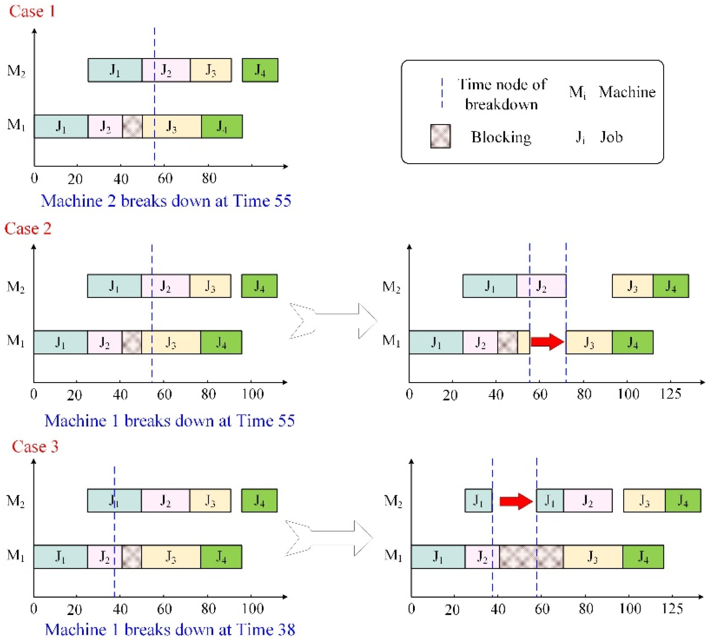
27] discussed both machine breakdown and processing change interruptions for a hybrid flowshop. The authors have proposed a hybrid fruit fly optimization algorithm (HFOA) with processing-delay, cast-break erasing, and right-shift strategy to minimize different rescheduling objectives in a steelmaking-foundry system. Li et al. [28] also considered five types of interruption events in the flowshop, namely machine breakdown, new jobs arrival, jobs cancellation, job processing change, and job release time change. A rescheduling strategy based on job status was designed for each event. A discrete teaching and learning optimization (DTLO) algorithm was proposed to optimize the makespan and stability. Valledor et al. [29] applied the Pareto optimum to solve the multi-objective flowshop rescheduling problem with makespan, total weighted tardiness, and steadiness as objectives. Three classes of disruptions (appearance of new jobs, machine faults, and changes in operational times) were discussed and an event management model was constructed. A restarted iterated Pareto greedy (RIPG) metaheuristic is used to find the optimal Pareto front.
From the above review, it can be concluded that current researches focused mostly on the rescheduling of a single flowshop with various constraints. Little literature has considered rescheduling from the distributed manufacturing perspective. Though the Industry 4.0 wireless networks [30,31] have quickly developed in recent years, they are involved more in distributed information interconnection rather than decision making in scheduling fields. Likewise, the big data-driven technology [32,33] may provide real-time decisions or schedule rules for small-scale manufacturing, but has not formed a sound system. Moreover, big data technology relies strongly on a large amount of historical data, it is difficult to apply to new products due to the highly discrete, stochastic, and distributed properties of scheduling problems. Therefore, with the in-depth application of distributed manufacturing, distributed rescheduling strategies and approaches need to be formulated prudently so that effective references could be provided for modern decision-makers.
On the other hand, the objects of job shop scheduling are usually individual jobs, products, or other resources in the manufacturing process. Such resources have typical discrete characteristics, which need to be marked and expressed through special information carriers, and then obtain new combinations (ranking) by constantly updating the information carriers. These optimization characteristics are similar to the optimization process of the intelligent algorithm based on the permutation model. Therefore, the intelligent algorithm based on the evolution concept is more suitable for solving scheduling problems.
According to the above analysis and good applicability of the intelligent algorithm, we use an intelligent algorithm to reschedule the distributed blocking flowshop scheduling problem in a dynamic environment (DDBFSP). In the last decade, the application of intelligent algorithms for solving scheduling problems has been extensively investigated. Memetic algorithm (MA), also called the Lamarckian evolutionary algorithm, is attracting increasing concern. The concept of “meme” refers to contagious information patterns proposed by Dawkins in 1976 [34]. “Memes” are similar to genes in GA, but there are differences: Memetic evolution is characterized by Lamarckism, while genetic evolution is characterized by Darwinism. Meanwhile, neural system-based memetic information is more malleable than genetic information, so memes are more likely to change and spread more quickly than genes. In evolutionary computing, MA can combine various global and local strategies to construct different search frameworks, which possess the characteristics of GA but with stronger merit-seeking ability. MA was widely applied in many engineering problems, such as vehicle path planning [35], home care routing [36], bin packing problem [37], broadcast resource allocation [38], and production scheduling optimization [39,40,41]. Until now, MA has not been applied to solve DBFSP in a dynamic environment(DDBFSP), it will be of significance to extend MA as a solver for DDBFSP.
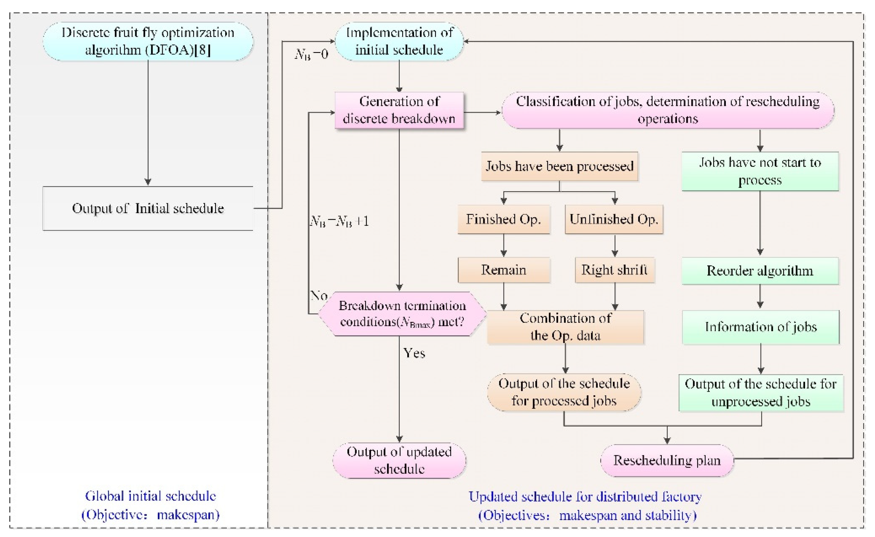
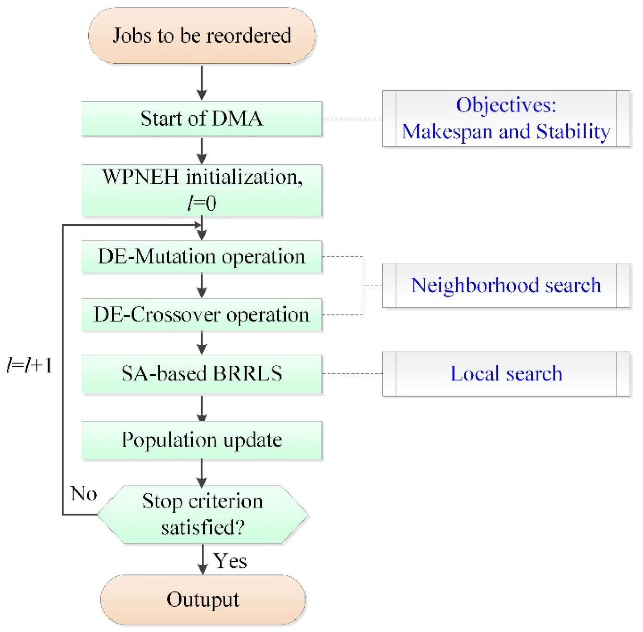
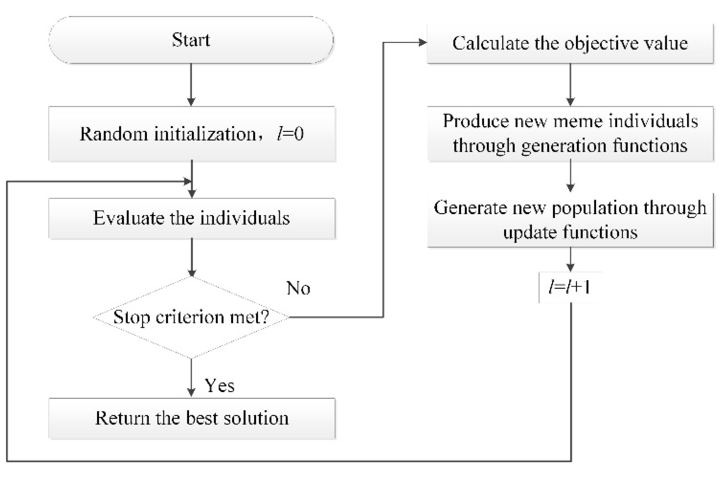
In summary, this paper aims to optimize DDBFSP with both makespan and stability measures as the objectives. The machine breakdown is defined as the disruption and assumed to happen stochastically in any distributed factories. To handle such dynamic events, a problem-specific disruption management model is constructed. A rescheduling framework that includes a job status-oriented classification strategy and a reordering algorithm-discrete Memetic algorithm (DMA) is proposed. For DMA, the differential evolution (DE) operators have been embedded to execute the neighborhood search. A simulated annealing (SA)-based reference local search framework is designed to help the algorithm escape from local optimums. Finally, the effectiveness of DMA is validated through comparative experiments. It is expected that the effect after rescheduling is to highly maintain the level of optimization of the original manufacturing objective (makespan) while ensuring the stability of the newly generated schedules.
The remainder of the paper is organized as follows. Section 2 states DDBFSP and constructs the mathematical model and objective function for DDBFSP. Section 3 designs the corresponding rescheduling framework. Section 4 elaborates the details of the DMA reordering algorithm. Section 5 verifies the performance of DMA and analyzes the results; Section 6 summarizes the research content of this paper.

2. Method

In this section, the mathematical models for DBFSP with optimization objectives in both static and dynamic environments are proposed. The classifications of job status after breakdown events are also introduced.

2.1. Statement of DBFSP in Static Environment

As can be seen in Figure 1, DBFSP not only needs to consider the correlation between processing task characteristics and blocking constraints but also needs to consider the coupling of global scheduling and local scheduling of each distributed factory, the solving process is more complex. As illustrated in Figure 1, a set of jobs J = { J j | 1 , 2 , , n } will be assigned to a set of factories F = { F k | k = 1 , 2 , , f } , each of which contains a set of machines M = { M i | 1 , 2 , , m } . The blocking constraint determines that no buffers are allowed between two adjacent machines. Therefore, the job can only be released to the next operation when the subsequent machine is free; otherwise, the job must be blocked on the current machine. We assume the processing time for each job is stochastic and different. After a job is assigned to a processing plant, it is not allowed to move to other factories.
Assume n k ( n k n ) jobs are assigned to factory k, and the job sequence in this factory is denoted as π k , where π k ( l ) represents the l - th job in π k . The operation O π k ( l ) , i has a processing time P π k ( l ) , i . Assume S π k ( l ) , 0 is the start time of π k ( l ) on the first machine of factory k, and d π k ( l ) , i is defined as the departure time of operation O π k ( l ) , i on machine i. The recursive formulas of DBFSP can be derived as follows:
S π k ( 1 ) , 0 = 0
D π k ( 1 ) , i = D π k ( 1 ) , i 1 + P π k ( 1 ) , i ,       i = 2 , 3 , , m
S π k ( l ) , 0 = D π k ( l 1 ) , 1 ,     i = 2 , , n k
D π k ( l ) , i = max { D π k ( l ) , i 1 + p π k ( l ) , i ,       D π k ( l 1 ) , i + 1 } ,       l = 2 , 3 , , n k       i = 1 , 2 , , m 1
D π k ( l ) , m = D π k ( l ) , m 1 + P π k ( l ) , m ,       l = 2 , 3 , , n k  
In the above equations, Equations (1) and (2) calculate the start and departure time of the first job π k from machine 1 to the last machine m in factory k. Equations (3) and (4) calculate the start and departure time of job π k ( l ) from machine 1 to machine m − 1. Equation (5) gives the departure time of π k ( l ) on machine m . If we take makespan C ( π k ) as the optimization objective, C ( π k ) of factory k can be expressed as:
C ( π k ) = D π k ( n k ) , m
As a result, the global makespan for DBFSP is defined through the comparison between C ( π k ) of all distributed factories:
C max ( Π ) = max k = 1 f ( C ( π k ) )
The detailed recursive process and example refer to our previous group work [8] for solving DBFSP.

2.2. Statement of DDBFSP

When characterizing the machine breakdown event of DBFSP in a dynamic and stochastic environment, the following questions should be marked: (1) Which factory has happened the breakdown event and when (the probability of breakdown)? (2) Which machine in that factory breaks (the distributivity of the breakdown)? (3) When will the machine resume?
In fact, machine breakdowns are difficult to simulate since the probabilistic model of breakdown occurrence could hardly cover the real manufacturing situation. Moreover, the recovery time is mostly predicted based on a priori knowledge, which cannot guarantee accuracy. With consideration of randomness and distribution, this paper triggers machine breakdowns in a randomly selected distributed factory at time t. The breakdown time is defined to follow a discrete uniform distribution function which is expressed as follows:
E ( B k , i ) = r a n d ( ) % P ( T i ) + p π k ( l ) × i ,         i = 1 , 2 , 3 , m ,   k = 1 , 2 , , f ,   l = 1 , 2 , , n k
where r a n d ( ) represents the random function between [ 0 , ω ] and ω denotes the maximum constant of the system; “%” is the remainder operator; P ( T i ) represents the total processing time of all jobs on machine i. Equation (8) defines the time range of the breakdown in the factory k during the processing time of all jobs, i.e., [ P π k ( l ) , i , C π k ( l ) , i ] .
To maintain the distribution of breakdowns and the convenience of experimental statistics, this study assumes that each distributed factory occurs β times random breakdowns during manufacturing. Additionally, to maintain the randomness of breakdown occurrence, each machine has the same probability to break down. To ensure a stochastic dynamic environment, the duration of breakdowns are generated randomly and uniformly following the interval [ 0 , ω ] and are determined immediately after the event. Moreover, other constraints for the breakdown event in DDBFSP are defined as follows:
(1)
All machines exist three statuses during manufacturing: idle, processing and blocked, a breakdown event occurs in the processing period.
(2)
The system triggers one machine breakdown each time, and the process stops immediately when the breakdown occurs.
(3)
After the machine is recovered, the affected process can continue with the remaining processing without re-processing.

2.3. Optimization Objectives of DDBFSP

In DBFSP, it is generally necessary to consider the production efficiency-related objective, e.g., makespan. While in a dynamic environment, from the decision point of view, stability becomes one importantly practical metric for manufacturing systems. If rescheduling optimization is performed only considering the production efficiency-related indicators, it may generate new schedules that deviate significantly from the initial plan, which in turn affects other planning activities, such as material management and manpower planning. Therefore, in the rescheduling phase, in addition to makespan, the stability of the new schedules should be considered. In this study, the initial schedule of one distributed factory before a breakdown occurs is denoted by B (Baseline), and the schedule after rescheduling is denoted by B * . The goal of rescheduling is to optimize both the makespan and the stability of the distributed factory at each breakdown node. The first objective (makespan) of the DDBFSP is expressed as follows:
f 1 = C max ( B * )
The second objective (stability) of the DDBFSP is derived as follows.
f 2 = min { i = 1 m l = 1 n k Z π k ( l ) , i } ,         k = 1 , 2 , , f ,   n k = 1 , 2 , , n
where the decision variable Z π k ( l ) , i indicates whether the relative position of the job B and B * has changed. Z π k ( l ) , i = 1 represents that the position of job π k ( l ) on machine i in factory k has changed in the new schedule B * and vice versa Z π k ( l ) , i = 0 .
To simplify the optimization process and avoid redundant calculations, a weighting mechanism is applied to combine both objective functions:
f ( B * ) = w 1 * f 1 + w 2 * f 2
In Equation (11), w 1 and w 2 represent the weight coefficients of f 1 and f 2 , respectively. Since f 1 and f 2 have different distribution ranges of dimensions, to avoid the results being dominated by the data with larger or smaller distribution ranges, the normalization method proposed in [24] is applied so that the value range of each objective falls in the interval. The normalization function is defined as follows:
f ( B * ) = w 1 * N ( f 1 ) + w 2 * N ( f 2 )
where:
N ( f 1 ) = f 1 ( B * ) l o w ( f 1 ) u p ( f 1 ) l o w ( f 1 )
N ( f 2 ) = f 2 ( B * ) l o w ( f 2 ) u p ( f 2 ) l o w ( f 2 )
In Equations (13) and (14), u p ( . ) and l o w ( . ) represent the upper and lower bounds of f 1 and f 2 for the two extreme rankings of the jobs at the breakdown node, respectively. The specific calculation procedure refers to [24].

2.4. Statement of Job Status after Breakdown Event

After a machine breaks down, the jobs are categorized to construct the event management model:
C π k ( l ) , i * S π k ( l ) , i * P π k ( l ) , i * + ( 1 y π k ( l ) , i , 1 ) ω 0
C π k ( l ) , i * S π k ( l ) , i * P π k ( l ) , i * ( 1 y π k ( l ) , i , 1 ) ω 0
C π k ( l ) , i * S π k ( l ) , i * P π k ( l ) , i * B e , i + B s , i + ( 1 y π k ( l ) , i , 2 ) ω 0
C π k ( l ) , i * S π k ( l ) , i * P π k ( l ) , i * B e , i + B s , i ( 1 y π k ( l ) , i , 2 ) ω 0
C π k ( l ) , i * max { S π k ( l ) , i * , B e , i } P π k ( l ) , i * + ( 1 y π k ( l ) , i , 3 ) ω 0
C π k ( l ) , i * max { S π k ( l ) , i * , B e , i } P π k ( l ) , i * ( 1 y π k ( l ) , i , 3 ) ω 0
g = 1 3 Y π k ( l ) , i , g = 1 ,         i = { 1 , 2 , , m } ,   k = { 1 , 2 , , f } ,   g = { 1 , 2 , 3 }
Y π k ( l ) , i , g = { 0 , 1 } ,           i = { 1 , 2 , , m } ,   k = { 1 , 2 , , f } ,   g = { 1 , 2 , 3 }
In the above equations, C π k ( l ) , i * denotes the completion time of job π k ( l ) on the machine i in B * . S π k ( l ) , i * and P π k ( l ) , i * represent the corresponding start time and processing time of C π k ( l ) , i * , respectively. B e , i and B s , i denote the occurrence time and completion time of the breakdown on the machine i . Equation (15) to Equation (20) defines three statuses in which an operation of a job is in when a breakdown occurs: Equations (15) and (16) determine that the operation was completed before the breakdown occurs; Equations (17) and (18) determine that the operation is being processed when the breakdown occurs; Equations (19) and (20) determine that the operation was originally scheduled to start after the machine is recovered. Equation (21) represents that the job can only be in a state in case a breakdown occurs. Equation (22) is a binary decision variable set for three cases: (1) Y π k ( l ) , i , 1 = 1 means the operation is completed before the breakdown occurs; (2) Y π k ( l ) , i , 2 = 1 denotes the operation overlaps with the machine breakdown node; (3) Y π k ( l ) , i , 3 = 1 means the operation begins after the machine is resumed.
For a better understanding, an example is presented in Figure 2 to illustrate the classification of the operation status at the moment that a machine breaks down. In case 1 of Figure 2, machine 2 of factory k breaks down at time 55, at which time the operations O π k ( 1 ) , 1 , O π k ( 1 ) , 2 and O π k ( 2 ) , 1 have already completed processing. Their start and completion times are not affected and do not need to be adjusted in the rescheduling phase. In case 2 of Figure 2, machine 1 breaks down at node 55 and operation O π k ( 3 ) , 1 is being processed at this time. The breakdown divides O π k ( 3 ) , 1 into two parts: the finished and the remaining part, the remaining part is completed after the machine is recovered. Hence, the start time O π k ( 3 ) , 1 remains unchanged in the rescheduling phase, but its finish time is affected by both the breakdown time and the recovery time. In case 3 of Figure 2, machine 1 breaks down at node 38 which is before the startup of job J 3 and J 4 . Therefore, the start and finish times of J 3 and J 4 are affected by both the breakdown time and the recovery time.

3. Rescheduling Framework for DDBFSP

Since the breakdowns occur during the manufacturing procedure, on which each job has already been fixed in a certain factory for processing, a change of jobs between different factories is unrealistic. Hence, the individual factory is defined as the decision subject in response to the events.

3.1. Rescheduling Strategy

We envision a stochastic and dynamic distributed scheduling environment. A two-stage “predictive-reactive” method is proposed for DDBFSP: initial solution pre-generation and rescheduling. In the first stage, the initial schedule for DDBFSP is generated by considering a static environment without machine breakdowns. After the breakdown occurs, the initial schedule may no longer be optimal. Therefore, in the second stage, the “event-driven” rescheduling is triggered to evaluate the breakdown, and a new schedule is provided in response to the events. Since the new schedule will be executed until the next breakdown occurs, the rescheduling strategy proposed in this study should have a dual objective: on one hand, to adapt and minimize the impact of the event; on the other hand, to generate a schedule that gives a good tradeoff between scheduling quality and stability when the event is resumed.

3.2. Rescheduling Method

According to the classification of operation status in Section 2.3, we propose a hybrid rescheduling method: “right-shift repair + local reorder”. At the breakdown node, no adjustment is made to the completed operations; for the directly affected operations, the right-shift strategy is adopted for a local repair; for the jobs that have not yet started their processing, the reordering algorithm is performed to seek a better partial schedule. The proposed “right-shift repair + local reorder” method is described as follows:
First, determine the jobs that are to be rescheduled. According to the constraint limitation of the flowshop manufacturing, once the processing sequence of the jobs on the first machine is determined, their sequence on other machines must be the same. Therefore, we mark the jobs π k ( l ) at the breakdown node by using the first machine as the reference. Suppose that there is a breakdown event at time B s , i when job π k ( l ) is processed on machine i, then the jobs in this factory of which the first operation has been started are counted in the set N c ; relatively, the jobs of which the first operation has not been started are counted in the set of unprocessed jobs N n .
Subsequently, the jobs N c are further divided by taking π k ( l ) as the midpoint: the jobs sequencing before π k ( l ) are included in the set N c , c = { π k ( 1 ) , , π k ( l 1 ) } ; the remaining jobs N c are included in the set N c , n . The rescheduling system maintains the same order and time points for the operations of jobs N c , c . For the operations of jobs in N c , n , the unaffected operations remain unchanged; the affected and other unprocessed operations are adjusted using the right-shift repair method [42], which shifts the start time to right by certain matching time units. The right-shift repair is essentially a FIFO-based heuristic.
At the breakdown node, all jobs N n have not been started processing. Their initial order may be no longer optimal after the recovery. Thus, we propose an improved algorithm to reorder the jobs. Eventually, the new schedule is merged into the global schedule and is executed as the baseline until the next breakdown occurs.
To describe the proposed “right-shift repair + local reorder” method more clearly, Figure 3 shows a comparative example with different rescheduling methods at the time of breakdown in one distributed factory. As shown in Figure 3a, the initial schedule of the factory has a desired makespan of 36. During manufacturing, Machine 2 breaks down at time B s , i = 8 and is assumed to be recovered at B e , i = 11 . At this point, the jobs that have already been processed on machine 1 are J 2 and J 1 (marked in gray), and these two jobs are counted in the set N c . In contrast, jobs J 3 , J 4 and J 5 are counted in N n . The framework adjusts the affected operations in N c based on the breakdown information and reorders the jobs in N n . As seen in Figure 3b, the right-shift method is implemented on partial operations of the jobs (marked in yellow), the process order remains the same as J 2 J 1 J 5 J 3 J 4 and the makespan is delayed to 41. In Figure 3c while using the “right-shift repair + local reorder” method, job J 3 , J 4 and J 5 (marked in green) is reordered using the reordering algorithm. The process order changes to J 2 J 1 J 3 J 4 J 5 and the makespan is 37, which absorbs 4 units of the recovery time. This example proves that the proposed rescheduling method is more efficient and flexible than the single rule-based (right-shift repair) heuristics.

3.3. Rescheduling Procedure

We illustrate the proposed optimization procedure for DDBFSP in Figure 4. First, with makespan as the optimization objective, a global schedule for DBFSP in a static environment is generated using DFOA [8]; then, each distributed factory executes manufacturing tasks according to their initial schedules; the breakdowns are triggered following the discrete generation mechanism proposed in Section 2.2. Each time the breakdown happens, rescheduling is implemented by the single distributed factory, with makespan and stability as optimization objectives. According to process status at the breakdown node, the jobs are classified and different methods (right-shift repair or reordering algorithm) are performed. The rescheduling results of different job sets are integrated, and the updated schedule under a single breakdown is provided as the initial schedule before the next event occurs. The above procedure is repeated until the termination condition of the breakdown trigger is met, and the final schedule is output.

4. Reordering Algorithm-DMA

Since the “right-shift repair” is introduced in [42], this section introduces the proposed reordering algorithm-DMA for the jobs in the set N n .

4.1. Introduction of Standard MA

MA was initially defined as an improvement of GA, it can combine different global and local strategies to construct various search frameworks, which has stronger flexibility, and merit-seeking ability than GA. The flow diagram of the basic MA is shown in Figure 5. MA starts from initializing the population, operates on memes with evolutionary thought, generates new individuals using generating functions (e.g., crossover and variation operators, etc.), and finally forms new populations using updating functions (e.g., selection operators, etc.).
Although standard MA has a strong optimization-seeking capability, it also encounters problems such as insufficient global exploration capability [43]. On the other hand, DE has proven its powerful search capability since being proposed. Inspired by this, we embed the DE operators into MA and proposed a discrete MA (DMA). DMA mainly contains the following parts: population initialization, DE (mutation and crossover), and local search.

4.2. Population Initialization

In the initialization phase, we use the well-known job sequence-based method [9] to encode. The position of each job in the sequence represents its processing order on corresponding machines. An initialization method WPNEH (Weighted position NEH method, WPNEH) considering the weighted position of the job is proposed under the premise of determining the reordering jobs.
Step 1: Using the PFT_NEH(x) heuristic [9] and the initial schedule to generate two seeds π P and π B . The total weighted position of a single job is defined as follows:
ϕ j = χ 1 × φ j ( π P ) + χ 2 × φ j ( π B )
In Equation (23), φ j ( π P ) and φ j ( π B ) represent the absolute positions of job j in two seeds. χ 1 and χ 2 represent the weight coefficients occupied by two seeds. The values of χ 1 and χ 2 are defined adaptively by the population size P s and the order l ( l = 1 , 2 , , P s ) of the newly generated individuals in the whole population:
χ 1 = l P s 1
χ 2 = 1 l P s 1
Step 2: Arrange all jobs in decreasing order of the total weighted positions ϕ j to obtain a sequence π 0 .
Step 3: Create a new empty sequence π e m p . The jobs in π 0 are inserted into each position π e m p in turn. The solutions obtained from each insertion are evaluated based on Equations (11) and (12) to determine the optimal order. Continue the operations until all jobs finish insertion.
Step 4: Let l = l + 1 , and continue steps 1–3 until all Ps individuals are generated.
The initialization procedure of WPNEH is shown as Algorithm 1.
Algorithm 1 WPNEH initialization
Input: job set N n , population size Ps, initial schedule B of a distributed factory
Output: initial population POP
01:  Define the order of jobs in N n , generate seed π B
02:  Apply PFT_NEH(x) method to rearrange the jobs in N n , generate seed π P
03:  While  l P s do
04:   Set the coefficient χ 1 = l / P s 1 and χ 2 = 1 l / ( P s 1 )
05:   Calculate ϕ j for each job according to Equation (22)
06:   Generate a new sequence π 0 by arranging all jobs in descending order based on their ϕ j
07:   Execute the NEH insertion procedure, evaluate the solutions obtained, find the best order
08:   Finish insertions of all jobs, obtain a new sequence π c , count in POP
09:    l = l + 1
10:  End While

4.3. DE Operation

DE [44] drives the search directions through the mutual synergistic and competitive behaviors among individuals of the population. Its overall structure is similar to GA, but the evolution principle is quite different. DE generates new individuals through perturbing the difference vectors of two or more individuals. It can obtain more operation space and enhance the global search capability when the individuals are significantly different from each other in the early stage of the search. In DMA, two key operators of DE (mutation and crossover) are embedded to perform the global search.

4.3.1. Mutation

The weighted difference vector of two individuals is first selected. Then, the weighted difference is summed with another individual vector. Hence, three individuals are randomly selected from the population POP, the optimal one is defined as π a , and the other two are defined as π b and π c . The mutation operator can be expressed as:
V a = π a κ ( π b π c )
where κ is the mutation scaling factor used to control the magnitude of the differences. “ ” represent the weighted differences between π b and π c :
π a π b = Δ δ ( j ) = { π b ( j ) ,       if   π b ( j ) π c ( j )   0 ,         otherwise j = 1 , 2 , , n
κ Δ = Φ φ ( j ) = { δ ( j ) ,       if   r a n d ( ) < κ   0 ,         otherwise
In Equations (27) and (28), Δ = [ δ ( 1 ) , δ ( 2 ) , , δ ( n ) ] and Φ = [ φ ( 1 ) , φ ( 2 ) , , φ ( n ) ] are the two temporary vectors used for the calculation. “ ” means the mutation individual π V is obtained through adding Φ with the target individual π b e s t :
π V = π b e s t Φ
The generation process of π V is described as follows.
Step 1: Select π a , set j = 1 .
Step 2: If φ ( j ) = 0 , set j = j + 1 , go to step 3; otherwise, generate a random number between (0, 1). If r a n d ( ) < κ , update π a by swapping the job π a ( j ) and φ ( j ) ; else, insert the job π a ( j ) into all different positions of φ ( j ) , take the optimal solution and update π a . Let j = j + 1 .
Step 3: If j n , return to step 2; otherwise, return π V = π a .
The mutation procedure of DMA is sketched in Algorithm 2.
Algorithm 2 Mutation Operation
Input: population POP, job number n, population size Ps, mutation factor κ , temporary set Δ and Φ
Output: mutation individual π V
01:  Select 3 individuals ( π a , π b and π c ) from POP randomly
02:   For  j = 1   to   n  do
03:    Calculate the vector difference δ ( j ) between two individuals and save in Δ
04:    Generate r a n d ( ) between (0,1), calculate the mutation difference φ ( j ) and save in Φ
05:   End For
06:   Output Φ
07:   For  j = 1   to   n do
08:    If  φ ( j ) = 0
09:      j = j + 1
10:    Else
11:     generate r a n d ( ) between (0, 1)
12:      If  r a n d ( ) < κ
13:       exchange job π a ( j ) and φ ( j ) in π a
14:      Else insert φ ( j ) from π a into all positions of after π a ( j ) , take the optimal solution
15:      End If
16:     return the π a
17:    End If
18:   End For
19:   Let π V = π a , output π V

4.3.2. Crossover

When solving discrete scheduling problems based on job sequence, the probability factor is mainly used to determine the crossed jobs [38]. In this study, we improved the determination method of the crossed jobs by eliminating the crossover probability factor and proposed a random crossover operator: First, select two jobs randomly from the mutated individual π V ; second, put these two jobs and jobs between them in a temporary set N t e m p ; third, determine the positions in π d of all jobs from N t e m p , remove all jobs from N t e m p and keep their positions. Finally, insert the jobs in π d with original order to obtain a new sequence π . The crossover process for π d is the same. When the crossover operation of the two parents is completed, the new individual obtained is evaluated and the best one is retained. The crossover operation is sketched in Algorithm 3.
Algorithm 3 Crossover Operation
Input: mutation individual π V , target individual π d , temporary job set N t e m p
Output: new individual π n e w
01: # Crossover operation on π d
02:  Select two jobs from π V randomly, put the jobs between them in N t e m p in turn
03:  Remove the jobs belonging to N t e m p from π d , keep the vacant position unchanged
04:  Insert the jobs in N t e m p into the free positions of π d to obtain the new solution π
05: # Crossover operation on π V
06:  Ensure π d has the job j N t e m p , clear N t e m p , put j in N t e m p orderly
07:  Remove jobs belonging to N t e m p from π V , keep the vacant position unchanged
08:  Insert the jobs in N t e m p into the free positions of π d to obtain the new solution π
09:  Evaluate new solutions:
10:   If f ( π ) < f ( π )
11:    Let π n e w = π , return π n e w
12:   Else
13:    Let π n e w = π , return π n e w
14:   End If
To facilitate understanding, Example 4-1 presents the procedure of DE operation in detail.
Example 4-1
Mutation: Three individuals are randomly selected from the initial population: π a = [ J 6 , J 3 , J 2 , J 4 , J 1 , J 5 ] , π b = [ J 1 , J 4 , J 6 , J 2 , J 5 , J 3 ] and π c = [ J 3 , J 4 , J 2 , J 1 , J 5 , J 6 ] . With Equation (26) it yields Δ = π b π c = [ J 1 , 0 , J 6 , J 2 , 0 , J 3 ] . A set of random numbers [ 0.7 , 0.6 , 0.9 , 0.4 , 0.1 , 0.3 ] are generated according to Equation (27), so that the mutation scaling factor is κ = 0.5 , then obtain Φ = [ 0 , 0 , 0 , J 2 , 0 , J 3 ] . It can be deduced that when j = 4 and j = 6 , there are φ ( 4 ) = J 2 and φ ( 6 ) = J 3 . For j = 4 , a random number 0.2 (<0.5) is generated between the interval (0,1) satisfying the uniform distribution. Then, two jobs π a ( 4 ) = J 4 and φ ( 4 ) = J 2 in π a are swapped and a new solution π a = [ J 6 , J 3 , J 4 , J 2 , J 1 , J 5 ] is obtained; for j = 6 , a random number 0.7 (>0.5) is also generated, the job φ ( 6 ) = J 3 in π a is inserted into the latter position of π a ( 6 ) = J 5 and a new solution π a = [ J 6 , J 4 , J 2 , J 1 , J 5 , J 3 ] is obtained.
Crossover: The mutation individual π V = [ J 6 , J 4 , J 2 , J 1 , J 5 , J 3 ] and the target individual π d = [ J 5 , J 3 , J 2 , J 4 , J 6 , J 1 ] are crossed as parents. First, two jobs J 2 and J 5 are randomly selected from π V , and set N t e m p = [ J 2 , J 1 , J 5 ] . For π d , remove the same jobs from N t e m p , obtain π d = [ X , J 3 , X , J 4 , J 6 , X ] . The new solution is obtained by reinserting N t e m p = [ J 2 , J 1 , J 5 ] into π d . The derivation of the new solution for π V is the same as π d , and the result is π V = [ J 6 , J 4 , J 5 , J 2 , J 1 , J 3 ] .

4.4. Job Block-Based Random Reference Local Search

As mentioned above, the two key operations of DE can improve the individuals concerning the vector difference of the population. Along with the iteration of an algorithm, the difference between individuals becomes smaller, which tends to lead the algorithm to local optimum easily. Therefore, DMA needs to equip with a local search framework to enhance its exploitation capability. For a long time, reference local search (RLS) has proved to be an effective local search algorithm and is often used to enhance the exploitation of metaheuristics [9]. RLS firstly generates a random reference sequence π r = [ π r ( 1 ) , π r ( 2 ) , , π r ( z ) ] , and uses it as a reference to guide the direction of the local search; subsequently, the jobs π r ( j ) are sequentially removed and inserted into all remaining positions of π r to obtain new solutions. The optimal solution is compared with the incumbent solutions of the population, and if it is better, it is replaced with the population. The insertion process is repeated until all the jobs are traversed. Though RLS has a strong local exploitation capability, it still has some problems. On one hand, RLS uses a single job insertion operation, which may destroy the good information of incumbent solutions and cause the loss of other good solutions. On the other hand, the fixed order of the reference sequence and the fixed insertion process of the jobs will result in a fixed path of local search. If π r ( j ) is constant for a long time, it will cause a large number of repeated searches, which directly affects the search efficiency of the algorithm.
Boejko et al. [45] have pointed out that in job sorting scheduling problems, compound moves (insertion and swap) based on the job block can retain excellent sequence information during the evolution of an algorithm. It thus expands the neighborhood structure and search space, which is better than single job insertion and swap operations. Inspired by this idea, we hybridize RLS and compound moves of job block, and propose a random reference local search based on job block (BRRLS): firstly, generate a reference sequence π r = [ π r ( 1 ) , π r ( 2 ) , , π r ( z ) ] randomly, where n r represents the number of jobs to be rescheduled; secondly, select two jobs J a and J b randomly, construct the job block (including J a and J b ) and take out all jobs in the individual π b l o c k that needs local search; then, insert the job block into all possible positions of π, evaluate the generated solutions, and select the optimal one. Repeat the above procedure (each time select two unselected jobs) until all jobs are traversed. The BRRLS process is sketched in Algorithm 4.
Algorithm 4 BRRLS Procedure
Input: job set N n , individual π, temporary set N t e m p , temporary set Λ
Output: new individual π n e w
01:  Randomly sort the jobs in N n to generate a reference sequence π r
02:  Randomly select two jobs J a and J b from N n
03:  Determine the block π b l o c k between J a and J b in π r (including J a and J b ) ,   save   π b l o c k in N t e m p
04:  Remove all jobs belonging to N t e m p from π
05:  Insert π b l o c k in all positions of π , evaluate and select the optimal solution, save in Λ
06:  Clear N t e m p ,   delete   J a and J b from N n
07:  Repeat the above operation (Line 03–07) until l e n ( N n ) 1
08:  Evaluate the individuals in Λ , return the optimal solution to π n e w
To further improve the algorithmic performance, a simulated annealing-like (SA) mechanism [46] is introduced as an acceptance criterion for BRRLS, which guides DMA to receive a certain percentage of poor solutions during the search to avoid being trapped in local optimums. The idea of SA is to compare the neighborhood solution π obtained by BRRLS with the incumbent solution π . If f ( π ) is better than f ( π ) , SA replaces π with π , otherwise, the decision of whether to accept π is based on a reception probability μ : A random number r a n d ( ) satisfying a uniform distribution is generated between ( 0 , 1 ) ; if r a n d ( ) < μ , π is replaced by the worse neighborhood solution obtained by the search. μ  is expressed as follows:
μ = e ( f ( π ) f ( π ) ) / T e m p
where Temp represents the temperature constant:
T e m p = T 0 j = 1 n k i = 1 m P π k ( l ) , i 10 × m × n , k { 1 , 2 , , f }
In Equation (31), T 0 is the temperature adjustment parameter preset by SA. It can be seen from Equation (31) that the closer f ( π ) is to f ( π ) , the closer the value μ is to 1 and π will be accepted with a higher probability. Conversely, if f ( π ) is much worse than f ( π ) , the value μ will be close to 0, and the solution π will be dropped with a higher probability. Hence, the SA-based reception mechanism ensures that the population does not deviate from the current search position, but can additionally absorb a certain percentage of non-quality solutions to avoid the algorithm from falling into local optimums.

4.5. Update Strategy of the Population

To maintain the diversity of individuals, the following strategy is applied to update the population: first, a new individual is generated using the mutation and crossover operators; subsequently, a local search is performed on these individuals, and the individuals are updated. finally, the incumbent solutions are replaced by the newly generated solutions, and the uniqueness of these new solutions is ensured to complete a single iteration of the whole population.

4.6. Flowchart of DMA

According to previous descriptions, Algorithm 5 presents the flowchart of DMA.
Algorithm 5 Flowchart of DMA
Input: population size Ps, mutation scaling factor κ , reordered job number n
Output: best solution π
01:  While termination condition not met do
02:   # Initialization (Section 4.2)
03:    Use WPNEH method to create new individuals
04:    Construct POP, evaluate the individuals
05:   # DE (Section 4.3)
06:    Perform DE according to κ ,   generate   P s / 2 individuals
07:    Perform random crossover operation on mutated individuals, and evaluate
08:   # BRRLS (Section 4.4)
09:    Implement the SA-based BRRLS procedure on the P s / 2 individuals
10:    Replace the incumbent solutions using solutions obtained by local search
11:    Update the population (Section 4.5)
12:  End While
The flow diagram of DMA is sketched in Figure 6. In general, DMA contains population initialization, DE operation, and local search. In the initialization phase, the population is generated using the WPNEH method; in the DE phase, the discrete differential mutation and crossover operators are executed to obtain the child individuals; in the local search phase, BRRLS is performed, and the simulated annealing mechanism is adopted as the reception criterion. Finally, the population is updated and the optimal solution is output.

5. Experimental Comparison and Analysis

5.1. Experimental Settings

Since few pieces of literature and public benchmarks have been developed for DDBFSP, we apply DFOA on its benchmark [8] to obtain test instances. These test instances are used as the initial schedules for each distributed factory. To fulfill different experimental requirements, the range of variable intervals of the DPFSP benchmark is set as n { 50 ,   100 ,   200 } , m { 5 ,   10 ,   20 } and f { 2 ,   3 ,   4 } . There are 27 combinations of different parameters, each containing 10 instances. The termination criterion of the algorithm is set to T max = 90 × n × m milliseconds.
The breakdown events are simulated according to the mechanism introduced in Section 2.2. When an event occurs on machine i, the trigger node is firstly limited to the interval [ P π k ( l ) , i , C π k ( l ) , i ] to ensure the timeliness of the breakdown. Since DMA performs only on partial jobs which have not started processing, we compress the breakdown interval to [ P π k ( l ) , i , C π k ( n k 2 ) , 1 ] , i.e., the start time of processing to the completion time of the penultimate job at the first machine, to ensure a feasible execution space for DMA.
The experiments are conducted on a PC with Intel(R) Core(TM) i7-8700 CPU and 16G RAM configuration, and the involved programs are compiled by Python. To balance the objective functions (makespan and stability), both weight coefficients w 1 and w 2 are set to 0.5. The algorithm is repeated 10 times for each breakdown in each factory, and the experiments use the average relative percent deviation (ARPD) as the metric to evaluate the mean quality of the obtained solutions. Since DMA is implemented for each distributed factory, the sum of ARPDs of all factories is firstly calculated, and the mean value is defined as the ARPD value for a single case of DDBFSP. The experiments will be conducted in the following three perspectives:
(1)
Key parameter calibration;
(2)
Effectiveness of the proposed optimization strategy;
(3)
Comparison with other intelligent algorithms.

5.2. Parameter Calibration

DMA contains three key parameters: population size P s , mutation scaling factor κ , and temperature adjustment parameter T 0 . The design of the experiment (DOE) [9] method is used for parameter calibrations, and in total 36 sets of initial schedules with factory number f = 3 were generated. The number of random breakdowns for each distributed factory is set to 2. The key parameters and ARPD values are defined as the control factors and response variables, respectively. The candidate values of the above parameters are set as: P s = { 30 , 50 , 80 , 100 } , κ = { 0.4 , 0.7 , 0.9 } and T 0 = { 0.1 , 0.2 , 0.3 , 0.4 } , which generate 48 configuration combinations. We use the “Analysis of Variance” (ANOVA) method to analyze the statistical results, as shown in Table 1.
As can be seen in Table 1, the p-values of P s , κ and T 0 are all less than 0.05 confidence level, which means all the parameters have important impacts on the performance of DMA. Among them, the corresponding F-ratio value of κ is the largest, which indicates that κ has the greatest impact on DMA. Moreover, Table 1 shows that the p-values of the interactions between every two parameters are greater than 0.05, which means the parameter interactions do not have a significant effect on DMA, and the parameter can be selected directly from the main effects plot in Figure 7.
From Figure 7, it can be observed that the performance of DMA decreases with the increment of κ , and DMA obtains the best results when κ = 0.4 . A relatively overlarge mutation scaling factor increases the randomness of search and leads to degradation of the mutation. The effect of P s ranks second, the performance of DMA first increases as the number of P s increases, it starts to decrease after reaching the optimum. This indicates that increasing P s appropriately will enhance the diversity of the population. However, an overlarge P s consumes too much running time of a single iteration, which in turn compresses the number of iterations and leads to a decrease in the probability of obtaining the optimal solution. The effect of T 0 on the algorithmic performance ranked the 3rd, and the main effect plot shows that the performance fluctuates with the growth of T 0 , DMA obtained the best results when T 0 = 0.4 . Based on the above analysis, the parameter combinations of DMA are set as: P s = 80 , κ = 0.4 , T 0 = 0.4 .

5.3. Effectiveness of the Proposed Algorithmic Component

DMA contains three important components: WPNEH initialization, DE operators, and BRRLS. To verify their effectiveness, we mask one corresponding part of DMA each time, and generate three types of variant algorithms from DMA: (1) DMA_RI: random initialization, which is used to verify the effectiveness of WPNEH initialization; (2) DMA_ND: without neighborhood search, which is used to verify the effectiveness of DE operators; (3) DMA_NL: without BRRLS, which is used to verify the effectiveness of BRRLS. The parameter settings and instances used in Section 5.2 were adopted. As the randomness of breakdown has a large impact on the results, to ensure the fairness of the comparison, only one complete set of breakdowns is simulated, and all variant algorithms are tested under this scenario. Table 2 shows the comparison results.
From Table 2, we can observe that the performance of DMA outperforms the other variants in all scenarios. In specific analysis, DMA outperforms DMA_RI, representing that the WPNEH initialization strategy can provide a better search starting point for DMA; DMA outperforms DMA_ND, indicating that the DE operators can improve the performance of DMA effectively. The results of DMA_NL are inferior to those of DMA, which means that the proposed BRRLS and SA-based reception criterion have an important influence on the optimization. BRRLS has retained the “greedy search” idea from RLS but improved the selection of jobs in the reference sequence. It ensures the inconsistency of local search step length through random selection of job blocks strategy, which makes the solutions obtained by local search more diverse and helps DMA to jump out of the local optimum. On the other hand, it can be observed from Table 2 that the differences between the compared algorithms are not significant when the scale of the instance is relatively small (e.g., n = 50 ). If the processing tasks (number of jobs) assigned to a distributed factory are small, the corresponding reorder execution space is also smaller, and the comparison algorithms are more likely to obtain optimal or suboptimal solutions in a given time. With the gradual increase in the problem size, the differences between algorithms start to manifest. The performance of each variant algorithm decreases more on the large-scale instances, while DMA remains relatively more stable.
To verify whether the differences were significant, we conducted a significance test from a statistical point of view. Each algorithm and ARPD value were chosen as the control variable and the response variable. Figure 8 demonstrates the mean plot of the 95% confidence interval. As can be seen, the ARPD values of each algorithm are ranked from top to bottom as DMA_ND, DMA_RI, DMA_NL, and DMA. The confidence intervals of each two algorithms do not overlap, which indicates that DMA is significantly better than its variants. The experimental results reveal that the proposed optimization strategies for each search phase jointly ensure the performance of DMA.

5.4. Comparison with Other Intelligent Algorithms

In this section, DMA is compared with the algorithms for solving traditional flow shop rescheduling problems. The compared algorithms are (1) Iterative Local Insertion Search (ILS) [25]; (2) Iterative Greedy Algorithm (IG) [25]; (3) Improved Migratory Bird Algorithm (IMBO) [47]; (4) Discrete Teaching and Learning Optimization (DTLO) Algorithm [29]. We follow strictly the literature to compile all the comparison algorithms, which share the same data structure, objective function, and termination criterion. To ensure comparison fairness, we apply the same rescheduling process, i.e., the comparison algorithms share the same initial schedules, the same time node distribution of breakdown events, and the same rescheduling strategy. The algorithms are only used to reorder unprocessed jobs as a way to test their optimization efficiencies. The calculation of ARPD is consistent with previous sections. The parameter combinations of the comparison algorithm were pre-adjusted and the specific settings are shown in Table 3. According to [25], as a single local search algorithm, ILS stops immediately after obtaining a local optimum, so no special parameters or termination conditions need to be set for ILS.
Table 4 shows the statistical results of different instances under single breakdown ( β = 1 ), the optimal values were bolded. It can be seen that DMA outperforms other algorithms in all instances of distributed scenarios. DTLO, IG, IMBO, and ILS obtain results in 2nd, 3rd, 4th and 5th place. It indicates that DMA is more suitable as a reordering algorithm. Specifically, ILS is an algorithm containing only a local insertion search framework, which lacks key structures such as population initialization and neighborhood search. It is difficult for ILS to balance exploration and exploitation, and therefore has the worst performance. As metaheuristics, DTLO, IG, and IMBO are more competitive in terms of performance on small-scale instances. For example, when the number of the distributed factory is set as f = 4 , and the total number of jobs is n = 50 , the results of other algorithms do not differ from DMA. The main reason is that when the size of the initial schedule is small, fewer processing tasks are assigned to each distributed factory. The search space for the solution becomes smaller, so the efficiency of each algorithm in finding the best solutions in a given time becomes high, thus reducing the variability of the comparison results. The same phenomenon is reflected in the scenarios of β = 2 and β = 3 , as shown in Table 5 and Table 6. DMA also performs the best among all comparison algorithms. As the number of breakdowns increases, the performances of the compared algorithms are not affected too much by small-scale instances. The performances on large-scale instances ( n = 200 ) showed different degrees of degradation. The errors of single rescheduling accumulate with the increment of breakdowns, which causes a deterioration effect, and thus decreases the algorithmic performances relatively. In comparison, the statistical results of DMA under different breakdown scenarios are less different, which also reveals that DMA is more stable and robust on both small- and large-scale instances.
To further verify the superiority of DMA, the differences between the compared algorithms are observed through statistical tests. ANOVA is used to describe the mean plot with a 95% confidence interval of the results obtained by the algorithms for different f, as shown in Figure 9.
It can be observed that the ARPD of DMA falls below that of other algorithms, and none of the confidence intervals overlap. It indicates again that the optimization performance of DMA is significantly better than its comparators. Moreover, it can be seen from Figure 9 that the performance of each algorithm gradually becomes better as f increases. This is mainly because the reordering algorithm does not focus on the assignment of jobs to plants in the initial schedule, rather on the reordering within the distributed factories. An increase in f leads to a decrease in assigned jobs and a corresponding decrease in their computational complexity and, therefore, an increase in the optimization-seeking efficiency of an algorithm.
Moreover, we compared and analyzed the performances under different numbers of breakdowns ( β ) based on the statistical results. Figure 10 shows the performance curves of the comparative algorithms. It can be seen that ARPD values increase as β gradually increases, representing that all the algorithms are affected by the frequency of breakdowns. Compared with other algorithms, ARPDs of DMA are improved by at least 88%. Moreover, ARPD values of ILS, IG, IMBO, and DTLO algorithms fluctuate more and show an increasing trend with the increase in β . Comparatively, ARPD values of DMA fluctuate the least, which indicates that the robustness of DMA under different scenarios is better than the compared algorithms.
In summary, DMA has a good performance for local reordering. Its innovation and advantages can be summarized as follows: (1) WPNEH initialization method provides a better initial population and high-quality search starting point for DMA; (2) the mutation and crossover operators based on DE provides an excellent neighborhood search capability; (3) BRRLS provides stronger local exploitation; (4) the SA-based reception criterion can help DMA jump out of the local optimum effectively. Among them, (2), (3) and (4) balance the exploration and exploitation of DMA.

6. Conclusions

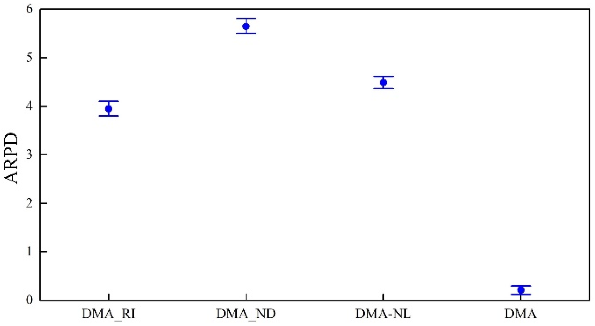
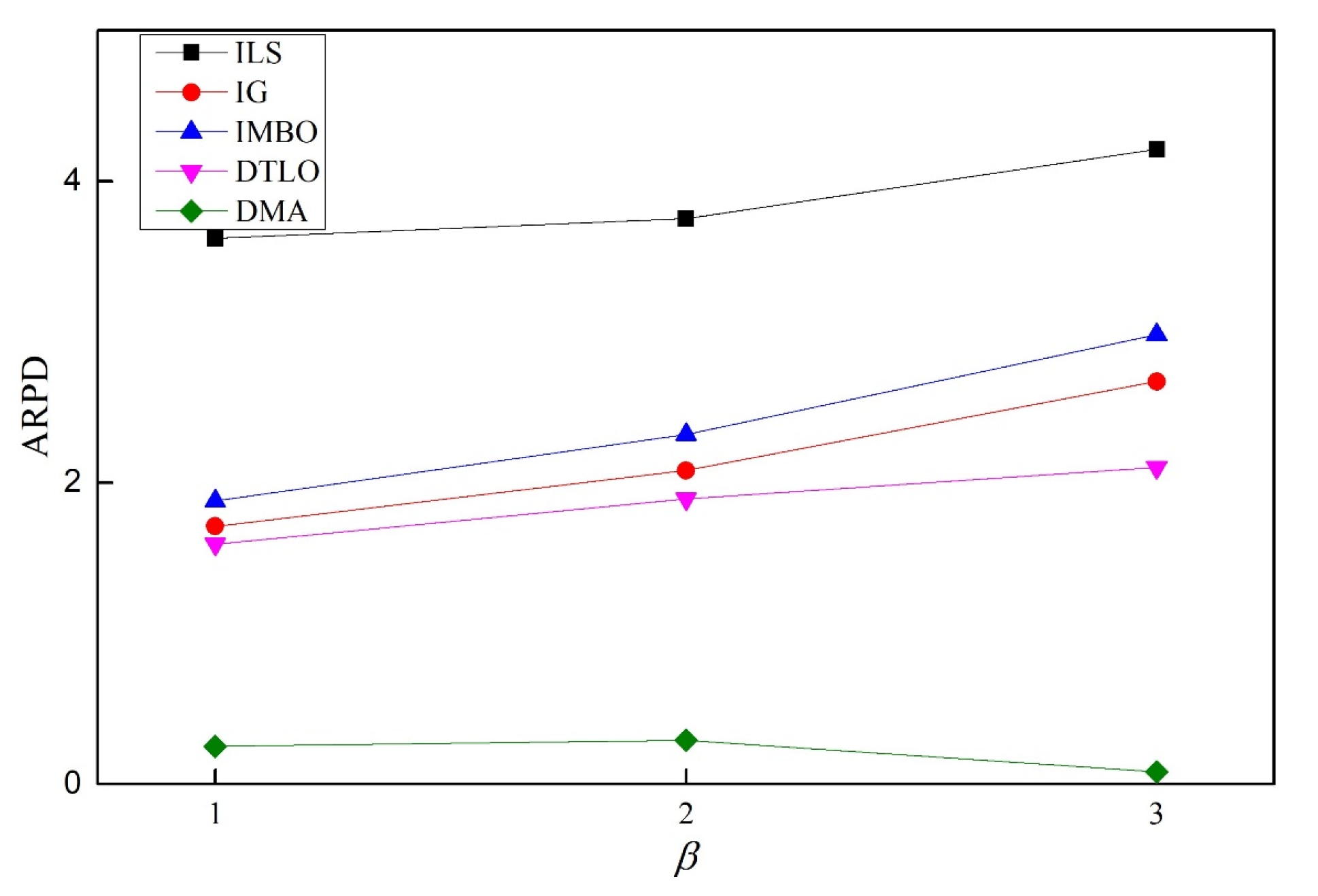
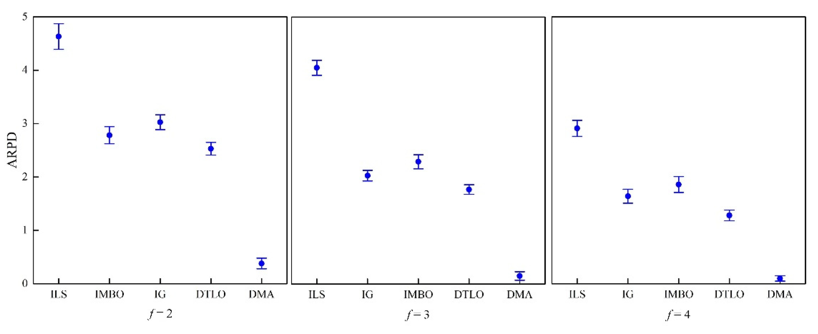
Building rescheduling optimization models and designing effective optimization methods according to the characteristics of distributed manufacturing are of significance to promote the research of the dynamic scheduling theory of distributed manufacturing. This study investigated the rescheduling strategy and algorithm for DDBFSP, in which machine breakdown events are considered as the disruption in the manufacturing site. Firstly, the mathematical model of DDBFSP including the event simulation mechanism is constructed. We consider makespan and stability as the objectives. The goal of this study is to optimize the bi-objective when the stochastic breakdown occurs in any distributed factories. We apply the “event-driven” policy in response to the disruption. A two-stage “predictive-reactive” rescheduling strategy is proposed. In the first stage, a static environment (DBFSP) without machine breakdown is considered, and the global initial schedules are generated; in the second stage, after machine breakdown occurs, the initial schedule is locally optimized by a hybrid repair policy based on “right-shift repair + local reorder”, and the DMA reordering algorithm based on DE is proposed for local reorder operation. For DMA, a WPNEH initialization method is designed to generate a high-quality population. In the neighborhood search phase, DE is embedded to improve the neighborhood structure and expand the target space by using mutation and crossover operators; in the local search phase, the BRRLS framework is proposed to perturb the high-quality solutions. To maintain the diversity, BRRLS has combined with the SA mechanism to receive the worse solutions with a certain probability. To obtain the best performance of DMA, the DOE method is used to calibrate three key parameters. The effectiveness of the proposed optimization strategy for DMA is verified through comparative experiments. Finally, DMA is compared with other algorithms on different test instances. The statistical analysis using ANOVA has verified the superiority of DMA.
Although the proposed rescheduling strategy has shown effectiveness, there still exist shortcomings. In this study, we only considered the breakdown event as the disruption. Real-life manufacturing suffers from far more than one disruption. The other common disruptions such as job cancellations and their interaction mechanism should be deeply investigated. Therefore, future works will concentrate on the construction of a more refined model that can manage more disruptions simultaneously.
This study attempts to explore the dynamic scheduling problem from the perspective of operational research optimization. With the development of the Industrial 4.0 network and big data, other artificially intelligent technologies play increasingly important roles in smart manufacturing. Combining data-driven technology with intelligent algorithms could adopt their respective advantages, and create more advanced optimization frameworks. For example, intelligent optimization can provide a large amount of historical scheduling data, which can be aggregated with other industrial information as a sample source for data-driven and machine learning. Therefore, the scheduling decision-making function can be deployed hierarchically and decoupled according to different scenarios and environments, thus making rational use of computing resources and improving the flexibility and stability of the system.

Author Contributions

Conceptualization, Z.L.; methodology, X.Z.; software, Y.H.; validation, Z.L., X.Z. and M.R.; formal analysis, G.K.; investigation, R.S.; resources, G.K.; data curation, X.Z.; writing—original draft preparation, X.Z. and Y.H.; writing—review and editing, Z.L.; visualization, M.R.; supervision, G.K.; project administration, R.S.; funding acquisition, Z.L. All authors have read and agreed to the published version of the manuscript.

Funding

This research is funded by the Natural Science Foundation of Xuzhou, China (KC21070), National Natural Science Foundation of China (61803192), and the Narodowego Centrum Nauki, Poland (No. 2020/37/K/ST8/02748 & No. 2017/25/B/ST8/00962).

Data Availability Statement

All data can be requested from the corresponding author.

Conflicts of Interest

The authors declare no conflict of interest.

References

  1. Helu, M.; Sobel, W.; Nelaturi, S.; Waddell, R.; Hibbard, S. Industry Review of Distributed Production in Discrete Manufacturing. J. Manuf. Sci. Eng. 2020, 142, 110802. [Google Scholar] [CrossRef]
  2. Cheng, Y.; Bi, L.; Tao, F.; Ji, P. Hypernetwork-based manufacturing service scheduling for distributed and collaborative manufacturing operations towards smart manufacturing. J. Intell. Manuf. 2020, 31, 1707–1720. [Google Scholar] [CrossRef]
  3. Valilai, O.F.; Houshmand, M. A collaborative and integrated platform to support distributed manufacturing system using a service-oriented approach based on cloud computing paradigm. Robot. Comput.-Integr. Manuf. 2013, 29, 110–127. [Google Scholar] [CrossRef]
  4. Chen, S.; Pan, Q.K.; Gao, L. Production scheduling for blocking flowshop in distributed environment using effective heuristics and iterated greedy algorithm. Robot. Comput.-Integr. Manuf. 2021, 71, 102155. [Google Scholar] [CrossRef]
  5. Ribas, I.; Companys, R.; Tort-Martorell, X. Efficient heuristics for the parallel blocking flow shop scheduling problem. Expert Syst. Appl. 2017, 74, 41–54. [Google Scholar] [CrossRef] [Green Version]
  6. Ribas, I.; Companys, R.; Tort-Martorell, X. An iterated greedy algorithm for solving the total tardiness parallel blocking flow shop scheduling problem. Expert Syst. Appl. 2019, 121, 347–361. [Google Scholar] [CrossRef]
  7. Zhang, G.; Xing, K.; Cao, F. Discrete differential evolution algorithm for distributed blocking flowshop scheduling with makespan criterion. Eng. Appl. Artif. Intell. 2018, 76, 96–107. [Google Scholar] [CrossRef]
  8. Zhang, X.; Liu, X.; Tang, S.; Królczyk, G.; Li, Z. Solving Scheduling Problem in a Distributed Manufacturing System Using a Discrete Fruit Fly Optimization Algorithm. Energies 2019, 12, 3260. [Google Scholar] [CrossRef] [Green Version]
  9. Shao, Z.; Pi, D.; Shao, W. Hybrid enhanced discrete fruit fly optimization algorithm for scheduling blocking flow-shop in distributed environment. Expert Syst. Appl. 2020, 145, 113147. [Google Scholar] [CrossRef]
  10. Li, W.; Li, J.; Gao, K.; Han, Y.; Niu, B.; Liu, Z.; Sun, Q. Solving robotic distributed flowshop problem using an improved iterated greedy algorithm. Int. J. Adv. Robot. Syst. 2019, 16, 1729881419879819. [Google Scholar] [CrossRef] [Green Version]
  11. Zhao, F.; Zhao, L.; Wang, L.; Song, H. An ensemble discrete differential evolution for the distributed blocking flowshop scheduling with minimizing makespan criterion. Expert Syst. Appl. 2020, 160, 113678. [Google Scholar] [CrossRef]
  12. Miyata, H.H.; Nagano, M.S. The blocking flow shop scheduling problem: A comprehensive and conceptual review. Expert Syst. Appl. 2019, 137, 130–156. [Google Scholar] [CrossRef]
  13. Chen, Q.; Deng, L.-F.; Wang, H.-M. Optimization of multi-task job-shop scheduling based on uncertainty theory algorithm. Int. J. Simul. Model. 2018, 17, 543–552. [Google Scholar] [CrossRef]
  14. Liu, W.; Jin, Y.; Price, M. New meta-heuristic for dynamic scheduling in permutation flowshop with new order arrival. Int. J. Adv. Manuf. Technol. 2018, 98, 1817–1830. [Google Scholar] [CrossRef] [Green Version]
  15. Chen, J.; Wang, M.; Kong, X.-T.; Huang, G.-Q.; Dai, Q.; Shi, G. Manufacturing synchronization in a hybrid flowshop with dynamic order arrivals. J. Intell. Manuf. 2019, 30, 2659–2668. [Google Scholar] [CrossRef]
  16. Zhang, B.; Pan, Q.-K.; Gao, L.; Zhang, X.-L.; Peng, K.K. A multi-objective migrating birds optimization algorithm for the hybrid flowshop rescheduling problem. Soft Comput. 2019, 23, 8101–8129. [Google Scholar] [CrossRef]
  17. Moghaddam, S.-K.; Saitou, K. Predictive-Reactive Rescheduling for New Order Arrivals with Optimal Dynamic Pegging. In Proceedings of the 2020 IEEE 16th International Conference on Automation Science and Engineering, Hong Kong, China, 20–21 August 2020; pp. 710–715. [Google Scholar]
  18. Han, Y.; Gong, D.; Jin, Y.; Pan, Q. Evolutionary Multiobjective Blocking Lot-Streaming Flow Shop Scheduling With Machine Breakdowns. IEEE Trans. Syst. Man Cybern. 2019, 49, 184–197. [Google Scholar] [CrossRef] [PubMed]
  19. Nica, E.; Stan, C.-I.; Luțan (Petre), A.-G.; Oașa (Geambazi), R.-Ș. Internet of Things-based Real-Time Production Logistics, Sustainable Industrial Value Creation, and Artificial Intelligence-driven Big Data Analytics in Cyber-Physical Smart Manufacturing Systems. Econ. Manag. Financ. Mark. 2021, 16, 52–62. [Google Scholar]
  20. Popescu, G.-H.; Petreanu, S.; Alexandru, B.; Corpodean, H. Internet of Things-based Real-Time Production Logistics, Cyber-Physical Process Monitoring Systems, and Industrial Artificial Intelligence in Sustainable Smart Manufacturing. J. Self-Gov. Manag. Econ. 2021, 9, 52–62. [Google Scholar]
  21. Cohen, S.; Macek, J. Cyber-Physical Process Monitoring Systems, Real-Time Big Data Analytics, and Industrial Artificial Intelligence in Sustainable Smart Manufacturing. Econ. Manag. Financ. Mark. 2021, 16, 55–67. [Google Scholar]
  22. Vieira, G.-E.; Herrmann, J.-W.; Lin, E. Rescheduling manufacturing systems: A framework of strategies, policies, and methods. J. Sched. 2003, 6, 39–62. [Google Scholar] [CrossRef]
  23. Framinan, J.-M.; Fernandez-Viagas, V.; Perez-Gonzalez, P. Using real-time information to reschedule jobs in a flowshop with variable processing times. Comput. Ind. Eng. 2019, 129, 113–125. [Google Scholar] [CrossRef]
  24. Katragjini, K.; Vallada, E.; Ruiz, R. Flow shop rescheduling under different types of disruption. Int. J. Prod. Res. 2013, 51, 780–797. [Google Scholar] [CrossRef] [Green Version]
  25. Iris, Ç.; Lam, J.-S.-L. Recoverable robustness in weekly berth and quay crane planning. Transp. Res. Part B Methodol. 2019, 122, 365–389. [Google Scholar] [CrossRef]
  26. Ma, Z.; Yang, Z.; Liu, S.; Song, W. Optimized rescheduling of multiple production lines for flowshop production of reinforced precast concrete components. Autom. Constr. 2018, 95, 86–97. [Google Scholar] [CrossRef] [Green Version]
  27. Li, J.; Pan, Q.; Mao, K. A hybrid fruit fly optimization algorithm for the realistic hybrid flowshop rescheduling problem in steelmaking systems. IEEE Trans. Autom. Sci. Eng. 2016, 13, 932–949. [Google Scholar] [CrossRef]
  28. Li, J.; Pan, Q.; Mao, K. A discrete teaching-learning-based optimization algorithm for realistic flowshop rescheduling problems. Eng. Appl. Artif. Intell. 2015, 37, 279–292. [Google Scholar] [CrossRef]
  29. Valledor, P.; Gomez, A.; Priore, P.; Puente, J. Solving multi-objective rescheduling problems in dynamic permutation flow shop environments with disruptions. Int. J. Prod. Res. 2018, 56, 6363–6377. [Google Scholar] [CrossRef]
  30. Wade, K.; Vochozka, M. Artificial Intelligence Data-driven Internet of Things Systems, Sustainable Industry 4.0 Wireless Networks, and Digitized Mass Production in Cyber-Physical Smart Manufacturing. J. Self-Gov. Manag. Econ. 2021, 9, 48–60. [Google Scholar]
  31. Hamilton, S. Real-Time Big Data Analytics, Sustainable Industry 4.0 Wireless Networks, and Internet of Things-based Decision Support Systems in Cyber-Physical Smart Manufacturing. Econ. Manag. Financ. Mark. 2021, 16, 84–94. [Google Scholar]
  32. Riley, C.; Vrbka, J.; Rowland, Z. Internet of Things-enabled Sustainability, Big Data-driven Decision-Making Processes, and Digitized Mass Production in Industry 4.0-based Manufacturing Systems. J. Self-Gov. Manag. Econ. 2021, 9, 42–52. [Google Scholar]
  33. Pelau, C.; Dabija, D.-C.; Ene, I. What Makes an AI Device Human-Like? The Role of Interaction Quality, Empathy and Perceived Psychological Anthropomorphic Characteristics in the Acceptance of Artificial Intelligence in the Service Industry. Comput. Hum. Behav. 2021, 122, 106855. [Google Scholar] [CrossRef]
  34. Richard, D. The Selfish Gene; Oxford University Press: New York, NY, USA, 1976. [Google Scholar]
  35. Wang, J.; Zhou, Y.; Wang, Y.; Zhang, J.; Chen, C.; Zheng, Z. Multiobjective vehicle routing problems with simultaneous delivery and pickup and time windows: Formulation, instances, and algorithms. IEEE Trans. Cybern. 2015, 46, 582–594. [Google Scholar] [CrossRef] [PubMed]
  36. Decerle, J.; Grunder, O.; El Hassani, A.-H.; Barakat, O. A memetic algorithm for multi-objective optimization of the home health care problem. Swarm Evol. Comput. 2019, 44, 712–727. [Google Scholar] [CrossRef]
  37. Yancey, S.-K.; Tsvetkov, P.-V.; Jarrell, J.-J. A greedy memetic algorithm for a multiobjective dynamic bin packing problem for storing cooling objects. J. Heuristics 2019, 25, 1–45. [Google Scholar]
  38. Zhou, Y.; Fan, M.; Ma, F.; Xu, X.; Yin, M. A decomposition-based memetic algorithm using helper objectives for shortwave radio broadcast resource allocation problem in china. Appl. Soft Comput. 2020, 91, 106251. [Google Scholar] [CrossRef]
  39. Jiang, E.; Wang, L.; Lu, J. Modified multi-objective evolutionary algorithm based on decomposition for low-carbon scheduling of distributed permutation flow-shop. In Proceedings of the 2017 IEEE Symposium Series on Computational Intelligence, Honolulu, HI, USA, 27 November–1 December 2017; pp. 1–7. [Google Scholar]
  40. Abedi, M.; Chiong, R.; Noman, N.; Zhang, R. A multi-population, multi-objective memetic algorithm for energy-efficient job-shop scheduling with deteriorating machines. Expert Syst. Appl. 2020, 157, 113348. [Google Scholar] [CrossRef]
  41. Kurdi, M. An improved island model memetic algorithm with a new cooperation phase for multi-objective job shop scheduling problem. Comput. Ind. Eng. 2017, 111, 183–201. [Google Scholar] [CrossRef]
  42. Minguillon, F.E.; Stricker, N. Robust predictive–reactive scheduling and its effect on machine disturbance mitigation. CIRP Ann. 2020, 69, 401–404. [Google Scholar] [CrossRef]
  43. Deng, J.; Wang, L.; Wu, C.; Wang, J.; Zheng, X. A competitive memetic algorithm for carbon-efficient scheduling of distributed flow-shop. In International Conference on Intelligent Computing Lanzhou, China, 2–5 August 2016; Springer: Cham, Switzerland, 2016; pp. 476–488. [Google Scholar]
  44. Liu, X.; Zhan, Z.; Lin, Y.; Chen, W.; Gong, Y.; Gu, T.; Yuan, H.; Zhang, J. Historical and heuristic-based adaptive differential evolution. IEEE Trans. Syst. Man Cybern. Syst. 2018, 49, 2623–2635. [Google Scholar] [CrossRef]
  45. Boejko, W.; Grabowski, J.; Wodecki, M. Block approach-tabu search algorithm for single machine total weighted tardiness problem. Comput. Ind. Eng. 2006, 50, 1–14. [Google Scholar] [CrossRef]
  46. Osman, I.; Potts, C. Simulated annealing for permutation flow-shop scheduling. Omega 1989, 17, 551–557. [Google Scholar] [CrossRef]
  47. Duan, J.; Sun, W.; Li, J.; Xu, Y. A Flowshop rescheduling algorithm based on migrating birds optimization. Control. Eng. China 2017, 24, 1656–1661. (In Chinese) [Google Scholar]
Figure 1. An example of DBFSP with the Gantt chart.
Electronics 11 00249 g001
Figure 2. Classification of job status at machine breakdowns.
Electronics 11 00249 g002
Figure 3. Comparison of different rescheduling strategies.
Electronics 11 00249 g003
Figure 4. Proposed rescheduling procedure for DDBFSP.
Electronics 11 00249 g004
Figure 5. Flow diagram of standard MA.
Electronics 11 00249 g005
Figure 6. Flow diagram of DMA.
Electronics 11 00249 g006
Figure 7. Main effects plot of the parameters for DMA.
Electronics 11 00249 g007
Figure 8. Mean plots with 95% confidence intervals for DMA and its variant algorithms.
Electronics 11 00249 g008
Figure 9. Mean plot with 95% confidence interval of the compared algorithms on different scenarios.
Electronics 11 00249 g009
Figure 10. Performance comparison with different breakdown numbers.
Electronics 11 00249 g010
Table 1. ANOVA results of DMA parameter combinations.
SourceSum of SquaresDegree of Freedom Mean SquareF-Ratiop-Value
Ps38.4312.8134.40.007
κ 144.3272.2382.40.000
T 0 6.832.317.60.012
P s × κ 17.2962.98.80.354
P s × T 0 4.890.50.550.492
κ × T 0 0.560.12.460.087
Table 2. Comparison results between DMA and its variant algorithms.
InstanceARPD
n × m × fDMA_RIDMA_NDDMA-NLDMA
50 × 5 × 30.561.240.920.54
50 × 10 × 30.611.550.980.36
50 × 20 × 31.171.731.120.48
100 × 5 × 31.332.262.600.18
100 × 10 × 32.052.442.380.11
100 × 20 × 32.843.233.150.05
200 × 5 × 33.975.584.190.00
200 × 10 × 34.636.675.490.00
200 × 20 × 34.176.045.320.00
Table 3. Parameter determination of the compared algorithms.
AlgorithmParameters
ILS--
IGJob numbers of destruction 4
IMBOPopulation size 50; Neighborhood set size 7; Migratory birds pass on the number of solutions 3; Number of lead bird iterations 20; Number of population iteration 100; weighted factor 0.8
DTLOPopulation size 50; learning factor of teacher 1
Table 4. Comparison results of different algorithms by β = 1 .
Initial InstanceARPD
n × m × fILSIGIMBODTLODMA
50 × 5 × 22.401.461.431.061.02
50 × 5 × 32.180.550.850.510.39
50 × 5 × 40.000.000.000.000.00
50 × 10 × 22.931.771.481.131.08
50 × 10 × 32.460.720.830.660.28
50 × 10 × 40.140.000.000.000.00
50 × 20 × 23.171.041.471.191.05
50 × 20 × 32.890.851.040.690.34
50 × 20 × 41.740.310.490.000.00
100 × 5 × 24.232.532.282.240.53
100 × 5 × 33.441.561.711.470.17
100 × 5 × 42.561.421.381.250.08
100 × 10 × 24.492.062.332.090.58
100 × 10 × 33.231.601.631.710.22
100 × 10 × 42.911.531.241.390.13
100 × 20 × 25.442.552.702.310.32
100 × 20 × 33.691.971.801.880.04
100 × 20 × 43.281.111.311.780.37
200 × 5 × 25.782.883.532.900.00
200 × 5 × 34.952.192.612.130.12
200 × 5 × 44.162.282.392.110.08
200 × 10 × 25.573.543.723.020.06
200 × 10 × 35.112.052.472.000.00
200 × 10 × 44.392.292.452.030.00
200 × 20 × 26.062.983.843.230.00
200 × 20 × 36.082.572.791.970.00
200 × 20 × 44.472.562.942.190.00
Ave.3.621.711.871.590.25
Table 5. Comparison results of different algorithms by β = 2 .
Initial InstanceARPD
n × m × fLSIGIMBODTLODMA
50 × 5 × 22.891.661.821.450.83
50 × 5 × 32.060.410.520.280.25
50 × 5 × 40.000.000.000.000.00
50 × 10 × 23.041.771.841.500.98
50 × 10 × 32.110.320.630.260.13
50 × 10 × 40.220.000.000.000.00
50 × 20 × 23.281.741.901.560.95
50 × 20 × 32.040.360.610.330.21
50 × 20 × 41.650.550.530.000.00
100 × 5 × 23.552.762.872.510.68
100 × 5 × 33.791.841.971.590.19
100 × 5 × 42.741.711.691.280.84
100 × 10 × 23.922.662.752.440.55
100 × 10 × 33.721.931.931.640.31
100 × 10 × 42.631.581.821.350.67
100 × 20 × 24.732.852.922.670.41
100 × 20 × 33.961.852.051.780.18
100 × 20 × 43.041.661.921.200.23
200 × 5 × 26.124.034.734.090.12
200 × 5 × 36.583.043.672.820.05
200 × 5 × 44.162.843.042.550.08
200 × 10 × 26.494.394.544.150.00
200 × 10 × 36.713.053.442.960.00
200 × 10 × 44.392.653.452.910.13
200 × 20 × 26.884.454.964.320.00
200 × 20 × 36.333.583.702.710.00
200 × 20 × 44.472.433.492.630.00
Ave.3.752.072.331.880.29
Table 6. Comparison results of different algorithms by β = 3 .
Initial InstanceARPD
n × m × fLSIGIMBODTLODMA
50 × 5 × 21.800.580.730.390.20
50 × 5 × 32.010.340.640.280.15
50 × 5 × 40.000.000.000.000.00
50 × 10 × 22.931.701.881.470.11
50 × 10 × 32.170.450.700.300.24
50 × 10 × 41.310.000.000.000.00
50 × 20 × 23.282.012.031.920.06
50 × 20 × 31.940.630.780.440.17
50 × 20 × 41.590.240.430.000.00
100 × 5 × 24.373.043.152.830.05
100 × 5 × 33.652.192.242.020.19
100 × 5 × 42.932.112.181.850.00
100 × 10 × 24.622.963.292.890.52
100 × 10 × 33.982.732.812.500.28
100 × 10 × 43.152.062.861.720.00
100 × 20 × 25.893.123.562.840.13
100 × 20 × 34.713.173.373.010.06
100 × 20 × 43.442.882.941.560.00
200 × 5 × 26.614.094.913.470.00
200 × 5 × 36.234.615.232.980.00
200 × 5 × 46.163.774.531.930.00
200 × 10 × 26.794.614.863.540.00
200 × 10 × 36.474.875.653.940.00
200 × 10 × 46.574.194.292.200.00
200 × 20 × 26.845.125.274.070.00
200 × 20 × 36.975.435.194.830.00
200 × 20 × 46.213.984.842.580.00
Ave.4.162.632.942.040.08
Publisher’s Note: MDPI stays neutral with regard to jurisdictional claims in published maps and institutional affiliations.

