TB-NET: A Two-Branch Neural Network for Direction of Arrival Estimation under Model Imperfections

Abstract

For direction of arrival (DoA) estimation, the data-driven deep-learning method has an advantage over the model-based methods since it is more robust against model imperfections. Conventionally, networks are based singly on regression or classification and may lead to unstable training and limited resolution. Alternatively, this paper proposes a two-branch neural network (TB-Net) that combines classification and regression in parallel. The grid-based classification branch is optimized by binary cross-entropy (BCE) loss and provides a mask that indicates the existence of the DoAs at predefined grids. The regression branch refines the DoA estimates by predicting the deviations from the grids. At the output layer, the outputs of the two branches are combined to obtain final DoA estimates. To achieve a lightweight model, only convolutional layers are used in the proposed TB-Net. The simulation results demonstrated that compared with the model-based and existing deep-learning methods, the proposed method can achieve higher DoA estimation accuracy in the presence of model imperfections and only has a size of 1.8 MB.

1. Introduction

Direction of arrival (DoA) estimation has been widely studied in the fields of acoustics, radar, sonar, and wireless communication in the past few decades [1,2,3,4,5,6,7,8,9,10,11,12,13,14,15,16,17]. Traditional DoA estimation methods such as multiple signal classification (MUSIC) [1] and estimation of signal parameters via rotational invariance techniques (ESPIRIT) [2] rely on accurate signal models, and their DoA estimation accuracy may degrade significantly in the presence of model imperfections.

Recently, with the rapid development of deep learning, neural-network-based algorithms have been proposed for DoA estimation. Thanks to the data-driven characteristics, these methods can be robust against model imperfections [6]. Generally, these methods can be divided into those based on regression networks or classification networks.

Under regression networks, different structures have been proposed to estimate the DoA values. Specifically, an end-to-end algorithm was proposed in [7], and a deep convolutional network was used to recover the spatial spectrum in [8]. However, the network structure depends heavily on the number of sources, which makes it difficult to extend to the scenarios where the number changes. With a small number of snapshots, a neural network was utilized in [9] for signal denoising, and a deep neural network (DNN) was utilized in [10,11] to reconstruct the covariance matrix. In [12,13], bi-directional gated recurrent units (GRUs) and bidirectional long short-term memory (BiLSTM) were introduced to learn the dependencies of signals, and the DoAs were estimated by the regression layer. In [14], a DNN was proposed to map the received signals to those of a larger dimension, which can be equivalently considered as adopting an antenna array of a larger size such that the DoA resolution is improved.

For classification networks, the most common architecture is the grid-based model, which divides the angular domain into several sectors, and then, for each sector, it is determined whether there exists an incoming signal [15]. In [6], an autoencoder with multilayer classifiers was proposed to build the spatial spectrum. In [16], two frameworks were proposed to separate coherent signals. In [17], a deep convolutional neural network (CNN) with 2D convolutional layers was proposed to improve the DoA estimation accuracy under a low signal-to-noise ratio (SNR). The grid-based model can improve the training stability, and the structure is universal in scenarios where the source number changes, but it is difficult to achieve a high resolution due to the limited number of grids.

In this paper, we propose a grid-based two-branch neural network (TB-Net). In particular, the proposed classification branch (C-Branch) and regression branch (R-Branch) work in parallel and share a feature extraction network. The C-Branch provides a grid-based mask to coarsely determine the DoAs, and the R-Branch provides a refinement of the DoA estimates. At the output layer, the DoA estimates are obtained by combining the masks and the corresponding deviations. The sharing of the feature extraction network leads to a lightweight network. Besides, to further reduce the weight scale and computational complexity, the proposed TB-Net only consists of convolutional layers. The simulation results showed that compared with conventional classification networks, the proposed TB-Net can achieve higher DoA estimation accuracy at the small cost of the computational overhead. Additionally, compared with the model-based and existing deep-learning methods, TB-Net is more robust against model imperfections and requires less calculation.

The rest of this paper is organized as follows. In Section 2, the signal model and neural network are introduced. The proposed TB-Net is described in Section 3. Section 4 shows the simulation results. Section 5 concludes this paper.

2. Preliminaries

In this section, we first describe the signal model and then give a brief introduction about CNNs.

2.1. Signal Model

In this work, the narrow band signal was used for the training and testing. In addition, we took into account three kinds of model imperfections that can possibly degrade the DoA estimation performance.

Denoting $s_k\left(t\right)$ as the k-th incoming signal and ${\theta }_k$ as the DoA, the received signal can be expressed as:

$$\mathbf{x}\left(t\right)=\sum _{k=1}^K\mathbf{a}\left({\theta }_k\right)s_k\left(t\right)+\mathbf{n}\left(t\right),$$

(1)

where $\mathbf{n}\left(t\right)\sim CN(0,{\sigma }^2)$ is the Gaussian noise, K is the number of sources, and $\mathbf{a}\left({\theta }_k\right)$ is the array response vector. In this paper, we assumed that the uniform linear array (ULA) is adopted. Hence, we have:

$$\mathbf{a}\left({\theta }_k\right)=[1,e^{j2\pi \frac{d}{\lambda }sin\left({\theta }_k\right)},\cdots ,e^{j2\pi \frac{(M-1)d}{\lambda }sin\left({\theta }_k\right)}],$$

(2)

where M denotes the number of antennas in the ULA, d denotes the spacing between adjacent antennas, and $\lambda$ denotes the wavelength.

Similar to [6], we considered three kinds of model imperfections, i.e., gain and phase inconsistency ($e_g,e_{pha}$), inter-sensor mutual coupling ($e_m$), and the deviation of the antenna position ($e_{pos}$). Hence, the i-th ($i=1,\dots ,M$) element in $\mathbf{a}\left({\theta }_k\right)$ can be rewritten as:

$$\begin{array}{c}\hfill {\widehat{a}}_i\left({\theta }_k\right)=(1+e_m)(1+e_g)e^{j{e}_{pha}}{e}^{j2\pi \frac{e_{pos}+(i-1)d}{\lambda }sin\left({\theta }_k\right)}.\end{array}$$

(3)

2.2. Neural Network Model

The covariance matrix of $\mathbf{x}\left(t\right)$ can be approximated as:

$$\mathbf{R}=\frac{1}{N}\sum _{t=1}^N\left(\mathbf{x}\left(t\right)\times \mathbf{x}{\left(t\right)}^{*}\right),$$

(4)

where N denotes the number of snapshots. Then, the input to the proposed neural network is given by:

$$\mathbf{u}=\left[\mathrm{Vec}\right(\mathrm{Real}\left(\mathrm{Triu}\right(\mathbf{R}\left)\right)),\mathrm{Vec}(\mathrm{Imag}\left(\mathrm{Triu}\right(\mathbf{R}\left)\right)\left)\right)],$$

(5)

where $\mathrm{Triu}(·)$ represents the upper triangular area of the matrix and $\mathrm{Vec}(·)$ reformulates the matrix as a vector.

The convolutional layer has been widely used in neural networks, and the output of the i-th layer can be expressed as:

$${\mathbf{y}}_i=f\left(\underset{{\mathbf{v}}_i}{\underbrace{{\mathbf{W}}_i\times {\mathbf{u}}_i+{\mathbf{b}}_i}}\right),$$

(6)

where ${\mathbf{u}}_i$ is the input feature, ${\mathbf{W}}_i$ is the convolution kernel, and ${\mathbf{b}}_i$ is the bias. In (6), the non-linear function $f(·)$ (e.g., ReLU, Sigmoid, Tanh, etc.) is used for space mapping. To train the neural network, ${\mathbf{W}}_i$ is updated via backpropagation under a certain loss function [18].

To reduce the internal covariate shift and accelerate the convergence rate, batch normalization (BN) can be performed before activation [19], for which ${\mathbf{y}}_i$ can be rewritten as:

$${\mathbf{y}}_i=f\left(\frac{{\mathbf{v}}_i-E\left[{\mathbf{v}}_i\right]}{\sqrt{Var\left[{\mathbf{v}}_i\right]+ϵ}}\right).$$

(7)

3. Proposed TB-Net

Figure 1 shows the architecture of the proposed TB-Net, which can be divided into two parts: feature extraction network and parallel prediction network. The details of these two networks are represented in Section 3.1 and Section 3.2. The parallel prediction network consists of the C-Branch, the R-Branch, and an output layer, which are described in Section 3.2.1, Section 3.2.2 and Section 3.2.3.

The detailed parameters of TB-Net are listed in

Table 1. Parameters of the proposed TB-Net.

Network	Convolution Kernel (C_IN, C_OUT, H, W)	Stride	Activation and BN
Feature extraction network	(2, 8, 1, 5)	2	BN + ReLU
	(8, 32, 1, 5)	2	BN + ReLU
	(32, 64, 1, 5)	2	BN + ReLU
	(64, 128, 1, 5)	2	BN + ReLU
	(128, 128, 1, 3)	2	BN + ReLU
C-Branch	(128, 121, 1, 1)	1	Sigmoid
R-Branch	(128, 121, 1, 1)	1	Tanh

, where C_IN denotes the number of input channels, C_OUT denotes the number of output channels, H denotes the kernel height, and W denotes the kernel width.

3.1. Feature Extraction Network

The feature extraction network extracts features from the covariance matrix and outputs them to the C-Branch and R-Branch, which realizes feature reuse and reduces the computational complexity.

The parameters of the network were determined by experiments. The results showed that the network consisting of five convolutional layers had the best mean absolute error (MAE) performance, and the parameters of the convolution kernel in each layer are listed in Table 1. Additionally, BN was utilized to accelerate the convergence. The experiments showed that adopting BN in the first five layers led to the best training stability and the highest MAE accuracy.

3.2. Parallel Prediction Network

The prediction network consists of the C-Branch and the R-Branch, and these two networks work in parallel. Denoting G as the number of grids, the output of the C-Branch is a mask vector $\mathbf{m}=[m_1,m_2,\dots ,m_G]$ whose i-th element indicates the possibility that the DoA is around the i-th grid. The output of the R-Branch is a deviation vector $\mathbf{d}=[d_1,d_2,\dots ,d_G]$, where $d_i$ represents the DoA’s deviation, or estimation refinement, with respect to the i-th grid.

For model optimization, the total loss was set as:

$$L=0.1\times l_c+l_r,$$

(8)

where $l_c$ is the loss of the C-Branch and $l_r$ is the loss of the R-Branch.

3.2.1. Classification Network

In this paper, a source in the sector $[\theta -{0.5}^{\circ },\theta +{0.5}^{\circ }]$ ($\theta =-{60}^{\circ },-{59}^{\circ },\dots ,{60}^{\circ }$) was approximated by the grid $\theta$, and the result of the C-Branch is a vector with 121 elements, whose values belong to $\{0,1\}$. A coarse DoA estimation was obtained by the indexes of non-zero elements.

In the C-Branch, we used the Sigmoid function as the activation function of the output layer, which maps the result to [0, 1]. We used binary cross-entropy (BCE) as the loss function to optimize the neural network, i.e.,

$$l_c=\sum _{i=1}^G-(m_{i}log\left({\widehat{m}}_i\right)+(1-m_i)log(1-{\widehat{m}}_i)),$$

(9)

where $m_i$ is the label and ${\widehat{m}}_i$ is the output of the network.

3.2.2. Regression Branch

The proposed R-Branch consists of a convolutional layer containing 121 output channels, which is consistent with the C-Branch. For the i-th channel, the output is the deviation on the i-th grid in the C-Branch. Note that such a deviation is valid only when $m_i=1$.

Since the grid size in the C-Branch is $\Delta \theta$, the deviation is restricted within $[-0.5\Delta \theta ,0.5\Delta \theta ]$. Hence, the weighted Tanh function was used as the activation function, i.e.,

$$d_i=0.5\Delta \theta \times \mathrm{Tan}\mathrm{h}\left(v_i\right).$$

(10)

For training, we adopted $l_2$ as the loss function to optimize the neural network, i.e.,

$$l_r=\frac{1}{G}\sum _{i=1}^G{m}_i\times {(d_i-{\widehat{d}}_i)}^2,$$

(11)

where $d_i$ denotes the actual deviation and ${\widehat{d}}_i$ denotes the output of the R-Branch.

Most importantly, because the R-Branch is parallel with the C-Branch, there is no data dependency between the two networks, which implies that TB-Net can estimate the DoAs in one evaluation.

3.2.3. Output Layer

The output layer combines m and d and obtains the DoA estimates. It first finds K (the number of sources) peak indexes $\mathbf{p}=[p_1,\cdots ,p_k]$ in $\hat{\mathbf{m}}$ and obtains the coarse DoA estimation by multiplying the grid size. Then, a final DoA estimate is obtained by adding the deviations selected in d according to p. The process is shown as:

$$\begin{array}{c}\hfill {\widehat{\theta }}_k=\Delta \theta \times p_k+d_k,\end{array}$$

(12)

where ${\widehat{\theta }}_k$ denotes the DoA estimates and $\Delta \theta$ denotes the grid size.

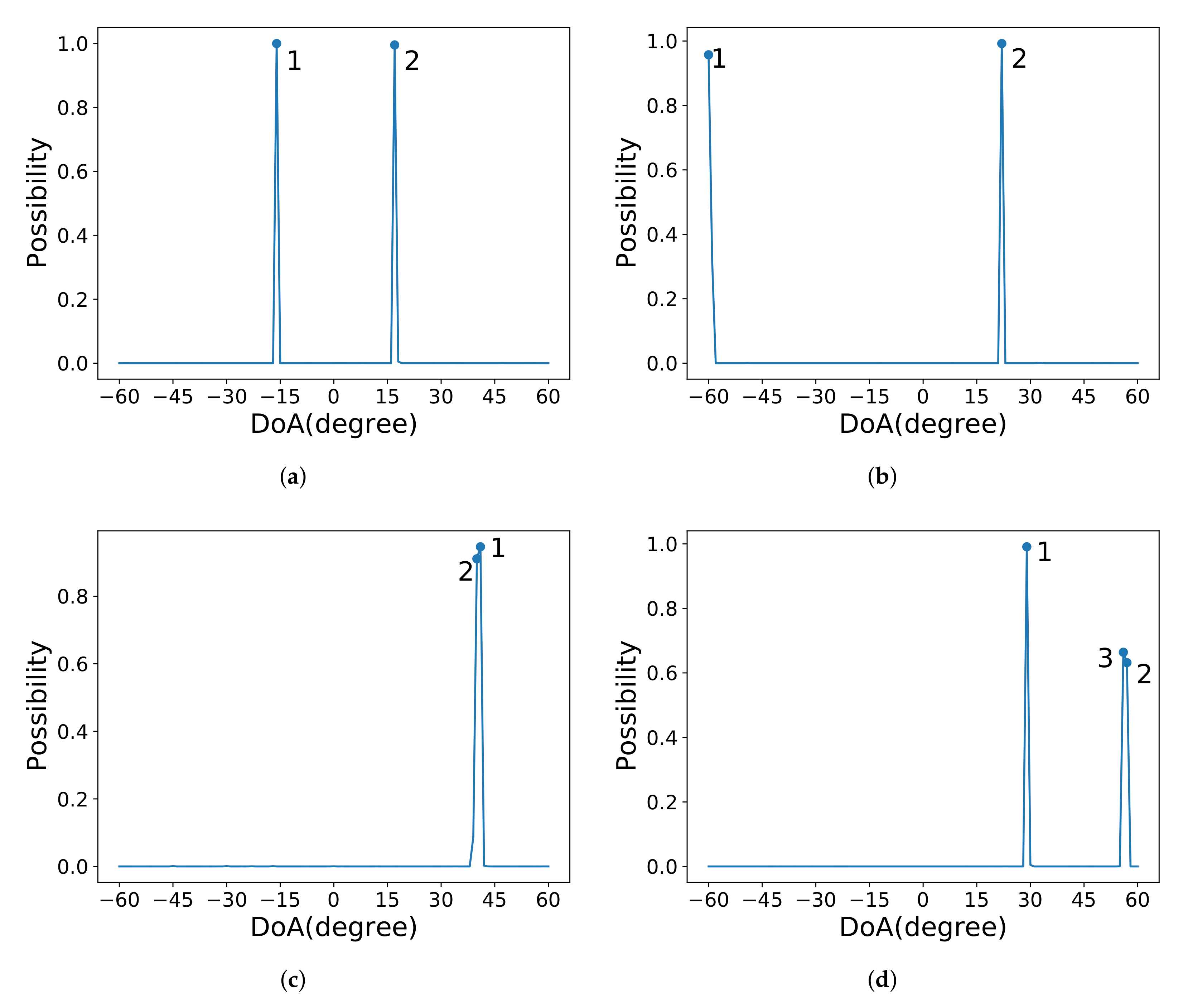
4. Experimental Results and Discussion

A 16-element ULA with a half-wavelength inter-element spacing was used to generate the dataset. Two sources with equal power were randomly generated within $[-{60}^{\circ },{60}^{\circ }]$. The scale of the dataset for training, validation, and testing was 100,000, 20,000, and 20,000, respectively.

We implemented TB-Net in Pytorch. In the training process, we set the initial learning rate to 0.001 and adjusted the learning rate every 30 epochs to 0.9-times the previous one. We used the Adam [20] optimizer to update the network parameters during training. The total training epoch was set to 300, and the candidate achieving the highest DoA estimation accuracy was selected as the final model.

We used MAE to measure the performance of the algorithms, i.e.,

$$MAE=\frac{1}{N_T}\sum _{i=1}^N(|({\theta }_1-{\widehat{\theta }}_1)|+|({\theta }_2-{\widehat{\theta }}_2)|),$$

(13)

where $N_T$ denotes the number of testing samples.

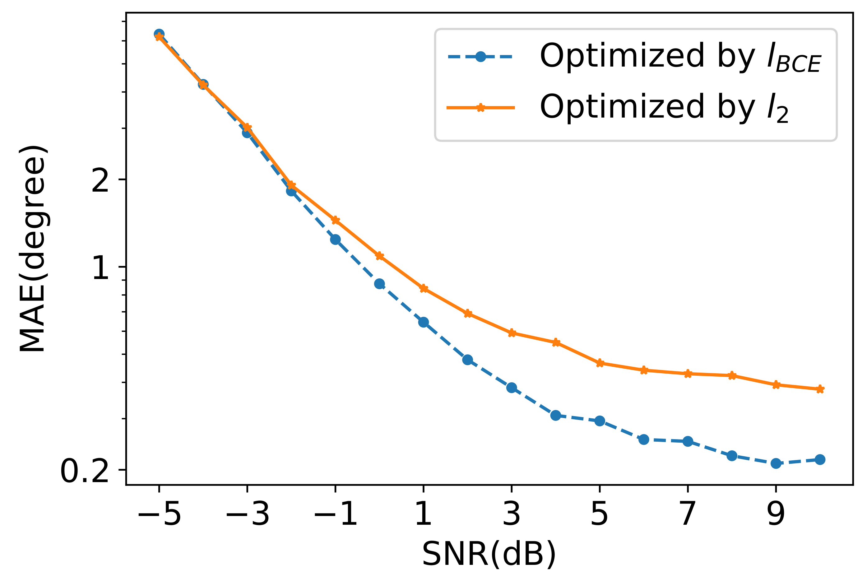
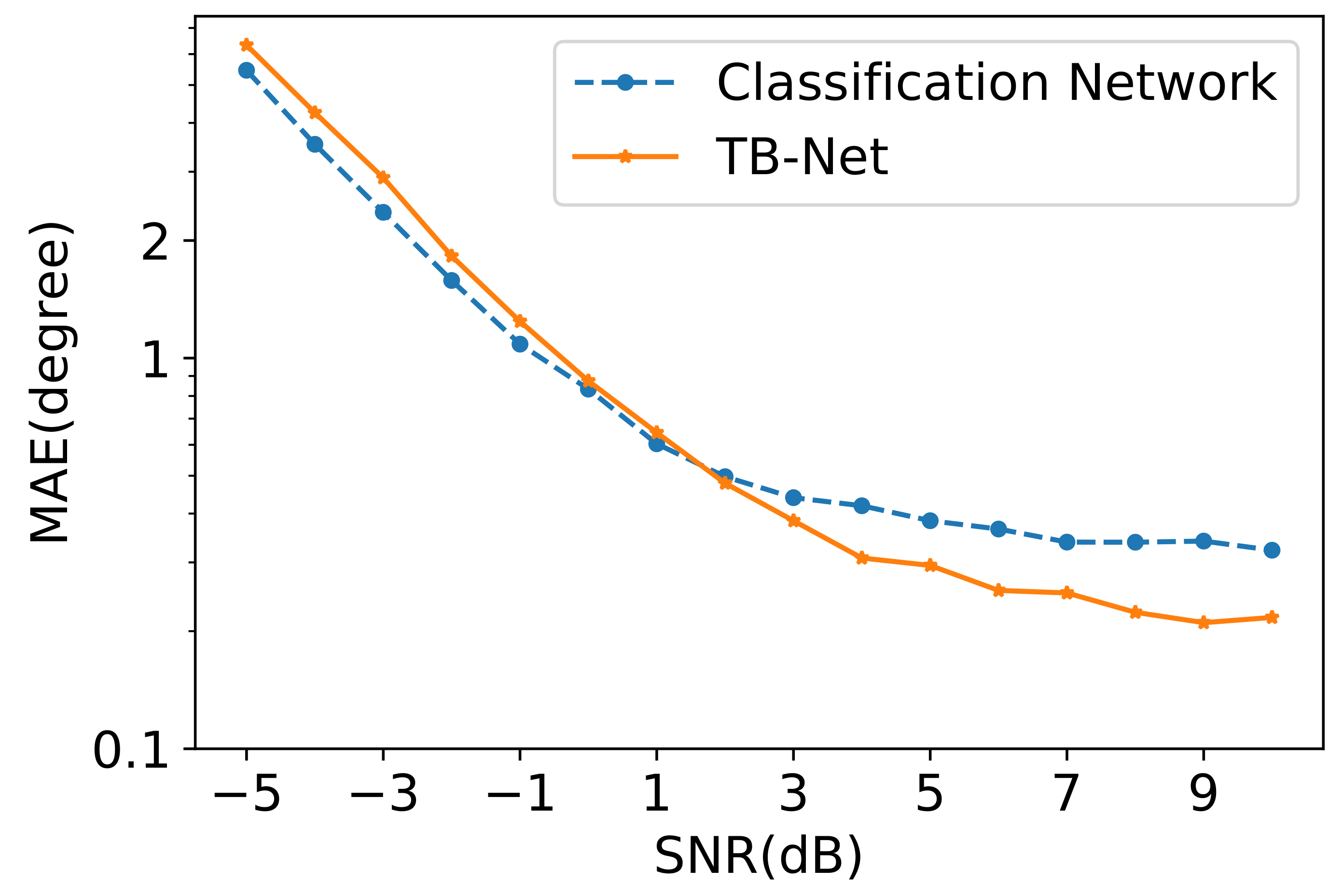
4.1. Experiments on TB-Net

4.1.1. Classification Network

As shown in Figure 2, the output of the C-Branch indicates the possibility of the source’s existence on the grids. In cases of (a), (b), and (c), the two grids corresponding to the peaks are considered as the DoA estimates. In the case of (d), the direction of ${56.47}^{\circ }$ causes closely located peaks on two grids, from which the one with the higher peak is taken as the DoA estimate (e.g., Point 3 in Figure 2d).

We compared the C-Branches that were optimized by $l_2$ and $l_{BCE}$ separately, and the results are shown in Figure 3. It can be seen that the network optimized by $l_{BCE}$ had a better accuracy than the one optimized by $l_2$. Under $\mathrm{SNR}=10\mathrm{dB}$, the improvement of the accuracy was about $44.7\%$.

4.1.2. TB-Net

Figure 4 shows the impact of the introduction of the R-Branch. It can be seen that the DoA estimation accuracy improved with SNR. When the SNR was low, the coarse estimates of the C-Branch were far from the DoA values and thus degraded the MAE significantly. With the increase of the SNR, the deviation given by the R-Branch gradually dominated the estimation accuracy, since the coarse DoA estimates obtained by the C-Branch almost had no error. This phenomenon was obvious when $\mathrm{SNR}>2\mathrm{dB}$. Compared with the C-Branch, TB-Net had an improvement of about $36.4\%$ in accuracy under $\mathrm{SNR}=10\mathrm{dB}$.

4.2. Complexity Analyses

The computational complexity comparison among DNN-based algorithms is listed in

Table 2. Computational complexity analyses.

Algorithm	DNN_SF_SS [6]	2D-CNN [17]	Proposed TB-Net
Weight (MB)	3.6	338.3	1.8
Calculation amount ($\times {10}^6$)	0.92	2.34	0.78

, where the weight denotes the model size and the calculation amount denotes the multiplication and addition operation number. We chose the networks proposed in [6,17] for comparison, which are briefly named DNN_SF_SS and 2D-CNN. The results implied that the CNN-based TB-Net had the minimum model size and computational complexity.

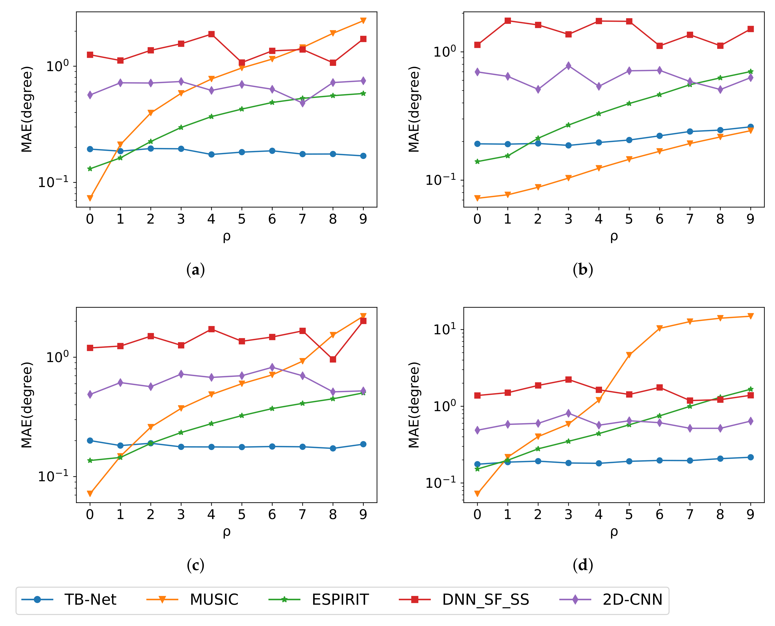
4.3. Experiments with Model Imperfections

The imperfections considered in this paper were modeled as:

$${\mathbf{e}}_g=0.1\times \rho \times [0,\underset{8}{\underbrace{0.2,\cdots ,0.2}},\underset{7}{\underbrace{-0.2,\cdots ,-0.2}}],$$

(14)

$${\mathbf{e}}_{pha}=0.1\times \rho \times [0,\underset{8}{\underbrace{-30,\cdots ,-30}},\underset{7}{\underbrace{30,\cdots ,30}}],$$

(15)

$${\mathbf{e}}_m=0.1\times \rho \times [0,{\gamma }^1,{\gamma }^2,\cdots ,{\gamma }^{15}],\gamma =0.3e^{j{60}^{\circ }},$$

(16)

$${\mathbf{e}}_{pos}=0.1\times \rho \times [0,\underset{8}{\underbrace{-1,\cdots ,-1}},\underset{7}{\underbrace{1,\cdots ,1}}],$$

(17)

where the parameter $\rho$ with value [$0.1,0.2,\dots ,0.9$] was used to control the strength of imperfections. For experiments, the data were generated under $\mathrm{SNR}=10\mathrm{dB}$, and the number of snapshots was set to $\mathrm{N}=40$.

We compared TB-Net with MUSIC [1], ESPIRIT [2], and DNN-based models. For MUSIC, the searching step was set to ${0.1}^{\circ }$. In order to make a fair comparison, the epochs of the training for TB-Net were set to 300. For the 2D-CNN and the DNN_SF_SS, the parameters used for the training were set according to [6,17].

Figure 5 shows that TB-Net performed well in all situations except the mutual coupling where MUSIC had the best performance. The prediction results of TB-Net did not fluctuate much with the increase of $\rho$, and the error was around ${0.19}^{\circ }$. In contrast, the performances of MUSIC and ESPIRIT deteriorated significantly with the increase of $\rho$, especially in the case of the gain and phase inconsistency and the deviation of the antenna position.

The error of the deep-learning-based algorithms did not deteriorate with the increase of $\rho$. However, the DNN_SF_SC [6] did not work well in all conditions, especially in inter-sensor mutual coupling. The MAE of the 2D-CNN [17] fluctuated around 0.6${}^{\circ }$, which was limited to the resolution of the grid-based classification network. In comparison, TB-Net constantly achieved high DoA estimation accuracy under various model imperfections.

5. Conclusions

In this paper, TB-Net, which combines classification and regression in parallel, was proposed to address DOA estimation. The DoA estimates were first coarsely obtained by the C-Branch and then further refined by the R-Branch. The experiments demonstrated that TB-Net had a higher DoA estimation accuracy in the presence of model imperfections. Besides, the C-Branch and the R-Branch shared a feature extraction network to reduce the model size. The convolutional layers were also adopted to implement a lightweight neural network. Hence, the proposed TB-Net had a model size of 1.8 MB and a calculation amount of 0.78 million, which is the minimum value to our knowledge. The proposed TB-Net has the limitation that the source number is assumed to be fixed and known. Therefore, the DoA estimation for an arbitrary source number is a potential direction for future research.

References

1. Schmidt, R.O. Multiple Emitter Location and Signal Parameter Estimation. IEEE Trans. Antennas Propag. 1986, 34, 276–280. [Google Scholar] [CrossRef] [Green Version]
2. Roy, R.; Kailath, T. ESPRIT-Estimation of Signal Parameters Via Rotational Invariance Techniques. IEEE Trans. Acoust. Speech Signal Process. 1989, 37, 984–995. [Google Scholar] [CrossRef] [Green Version]
3. Chen, P.; Yang, Z.; Chen, Z.; Guo, Z. Reconfigurable Intelligent Surface Aided Sparse DOA Estimation Method with Non-ULA. IEEE Signal Process. Lett. 2021, 28, 2023–2027. [Google Scholar] [CrossRef]
4. Chen, P.; Chen, Z.; Cao, Z.; Wang, X. A New Atomic Norm for DOA Estimation with Gain-Phase Errors. IEEE Trans. Signal Process. 2020, 68, 4293–4306. [Google Scholar] [CrossRef]
5. Chen, P.; Cao, Z.; Chen, Z.; Wang, X. Off-Grid DOA Estimation Using Sparse Bayesian Learning in MIMO Radar with Unknown Mutual Coupling. IEEE Trans. Signal Process. 2019, 67, 208–220. [Google Scholar] [CrossRef] [Green Version]
6. Liu, Z.; Zhang, C.; Yu, P.S. Direction-of-Arrival Estimation Based on Deep Neural Networks with Robustness to Array Imperfections. IEEE Trans. Antennas Propag. 2018, 66, 7315–7327. [Google Scholar] [CrossRef]
7. Hu, D.; Zhang, Y.; He, L.; Wu, J. Low-Complexity Deep-Learning-Based DOA Estimation for Hybrid Massive MIMO Systems with Uniform Circular Arrays. IEEE Wirel. Commun. Lett. 2020, 9, 83–86. [Google Scholar] [CrossRef]
8. Wu, L.; Liu, Z.; Huang, Z. Deep Convolution Network for Direction of Arrival Estimation with Sparse Prior. IEEE Signal Process. Lett. 2019, 26, 1688–1692. [Google Scholar] [CrossRef]
9. Papageorgiou, G.K.; Sellathurai, M. Fast Direction-of-arrival Estimation of Multiple Targets Using Deep Learning and Sparse Arrays. In Proceedings of the ICASSP 2020—2020 IEEE International Conference on Acoustics, Speech and Signal Processing (ICASSP), Barcelona, Spain, 4–8 May 2020; pp. 4632–4636. [Google Scholar]
10. Barthelme, A.; Utschick, W. A Machine Learning Approach to DoA Estimation and Model Order Selection for Antenna Arrays with Subarray Sampling. IEEE Trans. Signal Process. 2021, 69, 3075–3087. [Google Scholar] [CrossRef]
11. Barthelme, A.; Utschick, W. DoA Estimation Using Neural Network-Based Covariance Matrix Reconstruction. IEEE Signal Process. Lett. 2021, 28, 783–787. [Google Scholar] [CrossRef]
12. Barthelme, A.; Utschick, W. Robust DOA Estimation Method for MIMO Radar via Deep Neural Networks. IEEE Sens. J. 2021, 21, 7498–7507. [Google Scholar]
13. Adavanne, S.; Politis, A.; Virtanen, T. Direction of Arrival Estimation for Multiple Sound Sources Using Convolutional Recurrent Neural Network. In Proceedings of the 2018 26th European Signal Processing Conference (EUSIPCO), Rome, Italy, 3–7 September 2018; pp. 1462–1466. [Google Scholar]
14. Ahmed, A.M.; Thanthrige, U.S.K.P.M.; Gamal, A.E.; Sezgin, A. Deep Learning for DOA Estimation in MIMO Radar Systems via Emulation of Large Antenna Arrays. IEEE Commun. Lett. 2021, 25, 1559–1563. [Google Scholar] [CrossRef]
15. Liu, W. Super resolution DOA estimation based on deep neural network. Sci. Rep. 2020, 10, 19859. [Google Scholar] [CrossRef] [PubMed]
16. Xiang, H.; Chen, B.; Yang, M.; Xu, S. Angle Separation Learning for Coherent DOA Estimation with Deep Sparse Prior. IEEE Commun. Lett. 2021, 25, 465–469. [Google Scholar] [CrossRef]
17. Papageorgiou, G.K.; Sellathurai, M.; Eldar, Y.C. Deep Networks for Direction-of-Arrival Estimation in Low SNR. IEEE Trans. Signal Process. 2021, 69, 3714–3729. [Google Scholar] [CrossRef]
18. LeCun, Y.; Bengio, Y.; Hinton, G. Deep learning. Nature 2015, 521, 436–444. [Google Scholar] [CrossRef] [PubMed]
19. Ioffe, S.; Szagedy, C. Batch Normalization: Accelerating Deep Network Training by Reducing Internal Covariate Shift. In Proceedings of the International Conference Learning Representations (ICLR), San Diego, CA, USA, 7–9 May 2015; pp. 448–456. [Google Scholar]
20. Kingma, D.P.; Ba, J.L. Adam: A method for stochastic optimization. In Proceedings of the 3rd International Conference on Learning Representations, ICLR 2015, San Diego, CA, USA, 7–9 May 2015; pp. 1–15. [Google Scholar]
Figure 1. Architecture of the proposed TB-Net.
Electronics 11 00220 g001
Figure 2. The results of the C-Branch. The true directions of (ad) are ( 16.15 , 17.27 ), ( 59.92 , 21.92 ), ( 40.29 , 40.56 ), and ( 29.15 , 56.47 ), respectively.
Electronics 11 00220 g002
Figure 3. MAE comparison of the classification branch optimized by l B C E and by l 2 .
Electronics 11 00220 g003
Figure 4. MAE comparison of TB-Net and the C-Branch-based classification network.
Electronics 11 00220 g004
Figure 5. MAE comparison of the algorithms in the presence of different array imperfections: (a) combined imperfections, (b) mutual coupling, (c) deviation of antenna position, and (d) gain and phase inconsistency.
Electronics 11 00220 g005