Article

Electromagnetic Effective-Degree-of-Freedom Limit of a MIMO System in 2-D Inhomogeneous Environment

1
College of Information Science and Electronic Engineering, Zhejiang University, Hangzhou 310027, China
2
School of Electrical Engineering and Optical Technique, Nanjing University of Science and Technology, Nanjing 210094, China
3
School of Electronic Science and Engineering, University of Electronic Science and Technology of China, Chengdu 611731, China
4
School of Information and Communications Engineering, Xi’an Jiaotong University, Xi’an 710049, China
*
Author to whom correspondence should be addressed.
Electronics 2022, 11(19), 3232; https://doi.org/10.3390/electronics11193232
Submission received: 12 September 2022 / Revised: 3 October 2022 / Accepted: 6 October 2022 / Published: 8 October 2022

Abstract

:
Compared with a single-input-single-output (SISO) wireless communication system, the benefit of multiple-input-multiple-output (MIMO) technology originates from its extra degree of freedom (DOF), also referred to as scattering channels or spatial electromagnetic (EM) modes, brought by spatial multiplexing. When the physical sizes of transmitting and receiving arrays are fixed and there are sufficient antennas (typically with half-wavelength spacings), the DOF limit is only dependent on the propagating environment. Analytical methods can be used to estimate this limit in free space, and some approximate models are adopted in stochastic environments, such as Clarke’s model and Ray-tracing methods. However, this DOF limit in a certain inhomogeneous environment has not been well discussed with rigorous full-wave numerical methods. In this work, volume integral equation (VIE) is implemented for investigating the limit of MIMO effective degree of freedom (EDOF) in three representative two-dimensional (2-D) inhomogeneous environments. Moreover, we clarify the relation between the performance of a MIMO system and the scattering characteristics of its propagating environment.

1. Introduction

Based on the Shannon’s information theory [1], multiple-input-multiple-output (MIMO) technology in wireless communications has achieved great success over the last twenty years [2], along with the emerging massive [3], reconfigurable-intelligent-surface (RIS) [4,5] MIMO and holographic [6,7] MIMO systems. As electromagnetic (EM) wave is the physical carrier of information, the capacity bound of a space-constrained MIMO system from an EM perspective deserves to be investigated for exploring and examining the emerging MIMO technologies.
The degree of freedom (DOF) of a MIMO system refers to the rank (number of significant eigenvalues) of its correlation matrix [8], or the number of scattering channels [9] or spatial EM modes [10], which shows a clear physical meaning. DOF indicates the benefit brought by MIMO technology and is frequently used for characterizing the performance of a MIMO system. A more convenient figure of merit used in the MIMO system is the effective degree of freedom (EDOF) [11,12,13], which approximately characterizes its equivalent number of single-input-single-output (SISO) systems. The EDOF is directly related to the capacity and is easy to calculate.
The DOF/EDOF limit has been discussed in several research works, which can be roughly classified into mode-based and channel-based analyses. For the mode-based analysis, the DOF limit is intuitively calculated by counting the available EM modes in a constrained spatial or angular domain, including the DOF limit between two planes in free space [14], between one plane and half-space [15] and in Rayleigh environment [6,16,17]. For the channel-based analysis, the channel matrices are constructed with some empirical or EM methods, then the DOF/EDOF can be obtained through singular value decomposition (SVD), including the MIMO channels based on traditional models [18,19] (Clarke, Kronecker, etc.), EM Green’s function [20,21,22,23], full-wave simulation [24,25], and dyadic Green’s function in free space [13]. Particularly, the communication channels have been investigated with various EM methods, such as the numerical parabolic equations for tunnels [26], stochastic Green’s function for stochastic environments [27], ray-tracing methods [28] and some approximate models for the environment with finite scatterers [29,30,31,32]. These works provide some useful results for the DOF/EDOF of MIMO systems in free space and stochastic environments. Nevertheless, for some representative inhomogeneous environments, the impacts of their scattering characteristics on the performance of a MIMO system are not well investigated with numerical methods.
In this work, three main contributions are made. First, we provide an explicit deduction and explanation of the EM foundation of a MIMO system. Second, three representative numerical examples are given by using the two-dimensional (2-D) volume integral equation (VIE), the MIMO performances in these environments have not been discussed with EM numerical methods before. Third, the relation between the performance of a MIMO system and the scattering characteristics of the 2-D inhomogeneous environment is clarified. This paper demonstrates a simple but representative application of computational electromagnetic methods in wireless communications. The proposed model is particularly useful for evaluating and exploring the performance limit of MIMO systems in various deterministic environments which cannot be well modeled by empirical methods.

2. Methodology

2.1. EM Model for Analyzing EDOF Limit

If there are amounts of scatterers in the propagating environment, the strengths of signals going through this environment will follow a statistical model due to the central limit theorem, and the effect of specific physical properties, such as the size and shape of scatterers, are insignificant. These statistical models are generally applicable to various scenarios, which largely simplifies the modeling task of a communication system. However, for a few scatterers, these models are not applicable, and the scattering characteristics of the scatterers need to be taken into account with rigorous numerical methods.
We consider a general MIMO model in an isotropic inhomogeneous environment with homogeneous permeability μ and inhomogeneous permittivity ϵ ( r ) characterizing arbitrary scatterers, as depicted in Figure 1. A set of N S transmitting antennas at the positions r S n n = 1 , , N S are distributed in the source volume, N R receiving antennas at the positions r R m m = 1 , , N R are distributed in the receiving volume. The transmitting and receiving antennas are modeled as isotropic point sources/receivers, which is a widely-used approach for the DOF/EDOF analysis [10,13].
With source function J ( r ) , the resulting electric field is
E r = j ω μ G ¯ i n r , r J ( r ) d r ,
where G ¯ i n is the inhomogeneous dyadic Green’s function satisfying [33]
× × G ¯ i n r , r ω 2 μ ϵ ( r ) G ¯ i n r , r = I ¯ δ r r ,
with I ¯ the unit tensor. The matrix representation of G ¯ i n is
G ¯ i n = G x x G x y G x z G y x G y y G y z G z x G z y G z z ,
where each element is a scalar inhomogeneous Green’s function corresponding to one polarization of field and one polarization of source, denoted by its subscript. Under point source/receiver approximation, a channel matrix can be built for each scalar Green’s function. For G x y , a set of N S point sources at the positions r S n in the source volume are excited with the complex amplitudes t y n along the y polarization, then the superposed x-polarized electric field f x m generated at the positions r R m in the receiving volume would be
f x m = n = 1 N S G x y r R m , r S n t y n = n = 1 N S h m n t y n ,
where h m n = G x y r R m , r S n is the scalar inhomogeneous Green’s function with the pre-designed source and receiving positions. If t y n and f x m are collected in the two column vectors t y = [ t y 1 , t y 2 , , t y N S ] T and f x = [ f x 1 , f x 2 , , f x N R ] T , we can define the projection from the point sources to the point receivers as
f x = H x y t y ,
with the channel matrix
H x y = h 11 h 12 h 1 N S h 21 h 22 h 2 N S h N R 1 h N R 2 h N R N S .
Similarly, for full the polarizations in Equation (4), the complex amplitudes of sources t = [ t x t y t z ] T = [ t x 1 , , t x N S , t y 1 , , t y N S , t z 1 , , t z N S ] T is a 3 N S × 1 vector, and the complex amplitudes of received signals f = [ f x f y f z ] T = [ f x 1 , , f x N R , f y 1 , , f y N R f z 1 , , f z N R ] T is a 3 N R × 1 vector. The two column vectors are then related by a 3 N R × 3 N S EM channel matrix
H = H x x H x y H x z H y x H y y H y z H z x H z y H z z ,
where the nine N R × N S matrices correspond to the nine scalar inhomogeneous Green’s functions. The three polarizations of the electric field are orthogonal; hence, we could write the channel of full polarizations in a matrix form without loss of information. Notice that the (one-sample) correlation matrix R = H H or H H ( is the Hermitian operator) sharing the same eigenvalues is used for estimating the performance of a MIMO system, as the transmitting (receiving) powers are related by G ¯ i n G ¯ i n ( G ¯ i n G ¯ i n ).
The performance of a MIMO system can be characterized by the communication capacity, DOF and EDOF. Although capacity is an ultimate demand, we are focusing on the eigenvalues of the correlation matrix in this work, i.e., the influence of propagating environment, and the signal-to-noise ratio (SNR) can be considered as a constant. EDOF is used here for convenient calculation and comparison, as observing the significant eigenvalues for DOF is tedious. For a MIMO system, EDOF represents its equivalent number of SISO systems and can be calculated by [11]
Ψ e R = tr R R F 2 = i σ i 2 i σ i 2 ,
where tr ( · ) represents the trace operator, the subscript F denotes the Frobenius norm and σ i are the eigenvalues of R . This equation has been proved to be sufficiently accurate for estimating the performance of a MIMO system [13]. Generally, the EDOF limit is determined by both the size of the source/receiving volume and the propagating environment [20,21,22], and the latter is of concern here. With sufficient antennas (typically with half-wavelength spacings), the EDOF limit of a space-constrained MIMO system would be 1 in free space at the far field (line of sight) and reach the maximum value in the Rayleigh environment (rich scattering). When some scatterers are placed into the propagating environment to form an inhomogeneous environment, we will observe an increase in EDOF, which can be used for characterizing different inhomogeneous environments.

2.2. Numerical Method for Inhomogeneous Green’s Function

Based on Equation (5), when there are sufficient antennas, the performance limit of a space-constrained MIMO system is completely determined by the inhomogeneous Green’s function of the propagating environment, which can be investigated with full-wave numerical methods. As a proof of concept, and for a low computational cost, the 2-D VIE for the TM wave (only z polarization in Figure 2) is used for getting some fundamental results and gaining useful physical conclusions. Furthermore, various full-wave methods can be readily applied to corresponding scenarios following the framework proposed in Equations (4)–(8). For the TM wave case, the dielectric material is represented by equivalent polarization current J z ( x , y ) in VIE [34].
J z ( x , y ) = j ω ϵ 0 ϵ r ( x , y ) 1 E z ( x , y ) ,
where E z ( x , y ) is the total electric field, ϵ 0 is the permittivity in free space, and ϵ r is the relative permittivity. Then, the scattering problem can be modeled by
E z inc ( x , y ) = J z ( x , y ) j ω ε 0 ε r ( x , y ) 1 + j ω μ 0 A z ( x , y ) ,
where
A z ( x , y ) = J z x , y 1 4 j H 0 ( 2 ) ( k 0 R ) d x d y ,
and
R = x x 2 + y y 2 ,
k 0 is the free-space wavenumber, and H 0 ( 2 ) is the 2-D Green’s function in free space. After implementing spatial discretization in Figure 2 (N cells), we can use the 2-D pulse basis
p n ( x , y ) = 1 if ( x , y ) cell n 0 otherwise ,
the polarization current can be expressed as
J z ( x , y ) n = 1 N j n p n ( x , y ) .
Substituting the discrete current into the Equation (10) yields
E z inc ( x , y ) n = 1 N j n η p j k ε r ( x , y ) x , y ) 1 ] + j k η cell n 1 4 j H 0 ( 2 ) ( k R ) d x d y ,
which can be written into a matrix form
E z inc = Z ¯ J z ,
with the entries
E 2 inc x 1 , y 1 E 2 inc x 2 , y 2 · · · E z inc x N , y N = Z 11 Z 12 Z 1 N Z 21 Z 22 Z 2 N · · · · · · Z N 1 Z N 2 Z N N j 1 j 2 · · · j N ,
where
Z m n = k η 4 cell n H 0 ( 2 ) k R m d x d y m n ,
Z m m = η j k ε r m 1 + k η 4 cell m H 0 ( 2 ) k R m d x d y ,
R m = x m x 2 + y m y 2 .
The inverse of matrix Z ¯ is accelerated by the conjugate-gradient fast-Fourier-transform (CG-FFT) method [35,36]. By using the VIE, we can quickly calculate the field distribution excited by a point source at any position in arbitrary environments, thus obtaining the columns of the channel matrix. In fact, 2-D TM cases would be sufficient for gaining some fundamental EM insights, as many useful channel models are 2-D models, e.g., Clarke’s model [19].
For the specific setups, as shown in Figure 2, the distance between the source and receiving lines is D, the lengths of them are both L, and 2 L / λ 0 + 1 source/receiving points are uniformly distributed along the source/receiving lines (slightly smaller than 0.5 λ 0 spacings), which is sufficient for approaching the EDOF limit of a space-constrained MIMO system [6]. Arbitrary scatterers can be denoted by ϵ r ( x , y ) , for metallic structures, we use the complex permittivity of copper at 10 GHz ( ϵ r = 1 1.044 × 10 8 j ). The above would be the parameter settings for the following numerical examples.

3. Numerical Examples

3.1. Key-Hole Scenario

The key-hole scenario is a special and well-known MIMO system, where the rank of the correlation matrix is very low due to the particular propagating environment. Some approximate methods and experiments have been conducted for investigating this scenario [37,38]. Here, we present some results with the proposed model. The key-hole scenario discussed is shown in Figure 3a. A large metallic sheet with an aperture is set in the middle between the source and receiving lines, which becomes a key-hole scenario when the size of aperture (S) is very small. The lengths of the source and receiving lines are set relatively long ( L = D = 5 λ 0 ) so that there will still be EDOF gain when the sheet is removed. The relation between S and EDOF is depicted in Figure 3b. It can be observed that the EDOF will be gradually reduced to 1, i.e., become equivalent to that of a SISO system, when the size of the hole keeps decreasing. Moreover, the electric fields | E z | excited by a point source at position (−2.5, 0) with different S are demonstrated in Figure 4. When S = 0.5 λ 0 , less power could pass through the hole, and the field at the receiving line is rather uniform, which is not good for MIMO communication. More signals can be received and the field is more focused at the receiving line when S = 2 λ 0 .

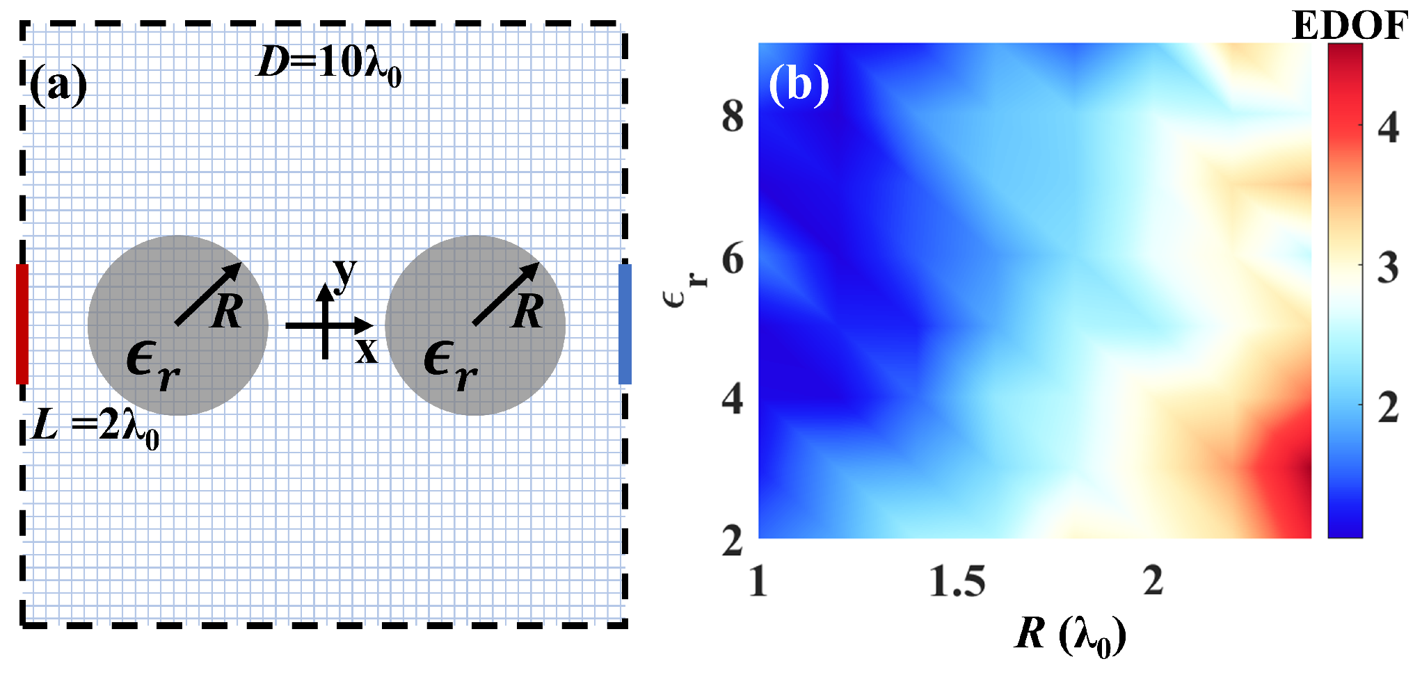
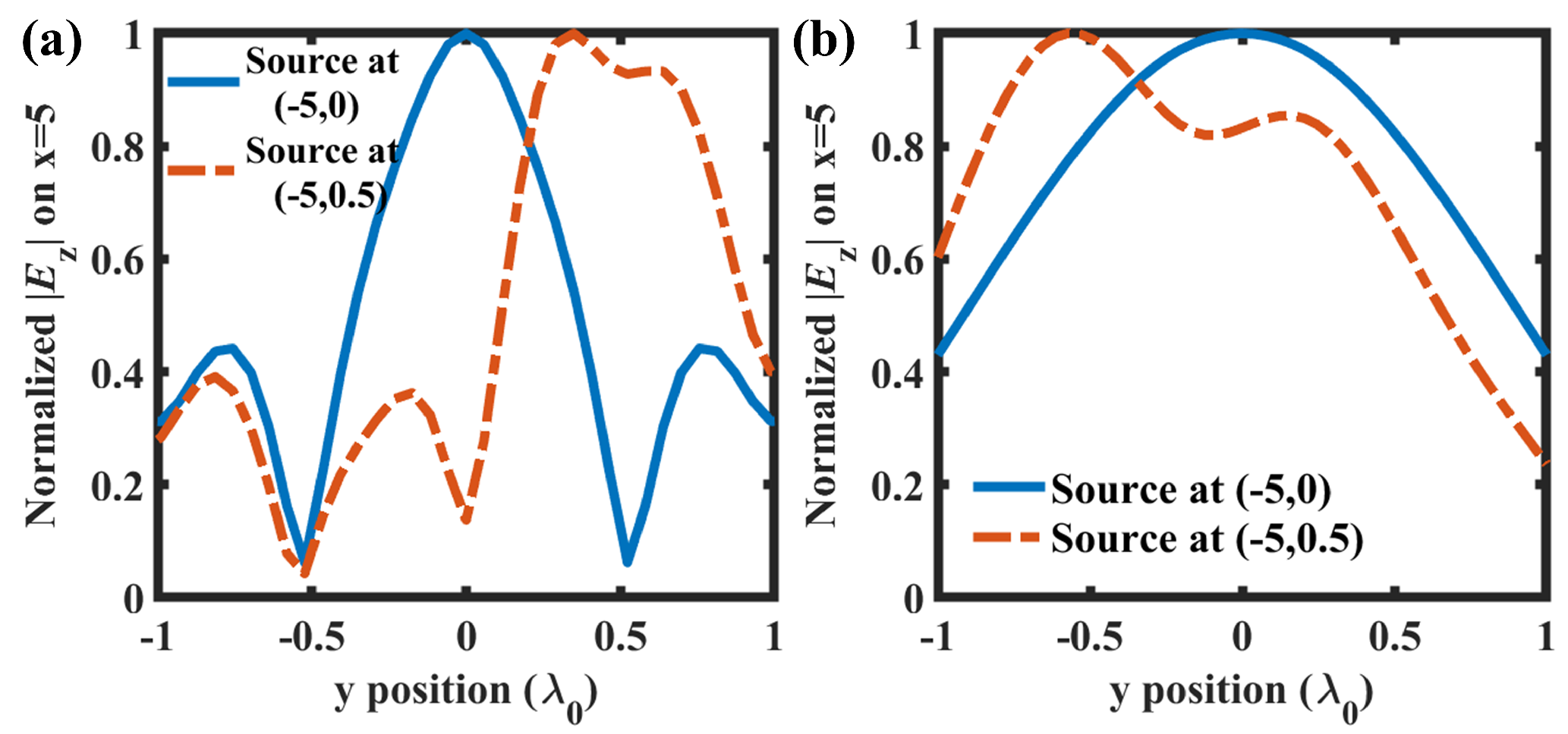
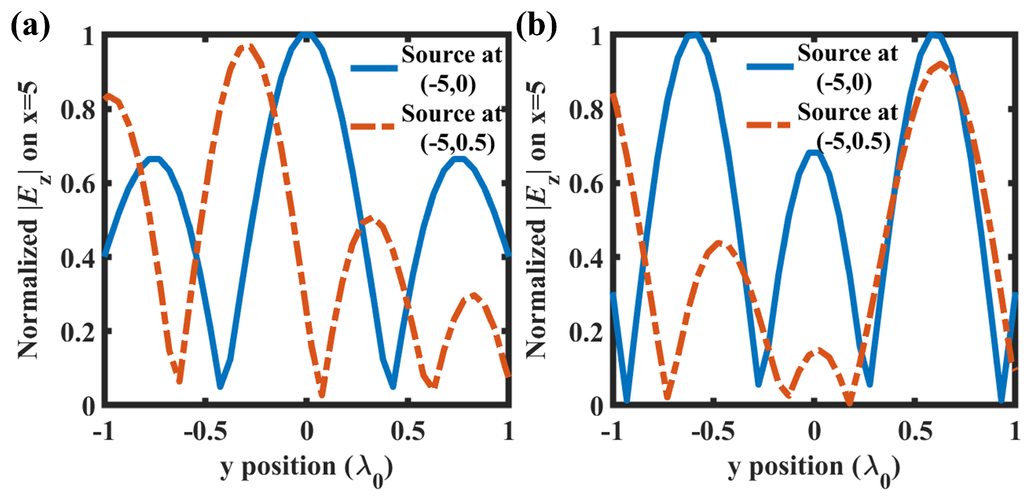
3.2. Cylindrical Scatterers

The EDOF limit in inhomogeneous environments constructed by 2-D cylindrical scatterers is also investigated. Here, we demonstrate a typical case after testing several kinds of combinations, including single, double, and uniform or random arrays of cylindrical scatterers. It has been found that the two-scatterer case depicted in Figure 5a can achieve relatively higher EDOF, where the two dielectric cylinders, with the same radius R and relative permittivity ϵ r , are placed in the left and right quadrisection points between the source and receiving lines. The lengths of the source and receiving lines are L = 2 λ 0 and the distance between them is D = 10 λ 0 , which fulfills the far-field condition (EDOF = 1 without the scatterers).
The EDOF versus R and ϵ r is shown in Figure 5b, from which we can observe that larger R can significantly improve EDOF, while the influence of ϵ r is not distinct. At the maximum value of EDOF (EDOF = 4.3), the cylindrical scatterers provide fairly good MIMO performance even close to that in a canonical Rayleigh channel (EDOF = 4.5). The normalized electric fields | E z | excited by point sources at positions (−5, 0) and (−5, 0.5) in the best case ( R = 2.4 λ 0 , ϵ r = 3 ) are depicted in Figure 6a, and that in the worse case ( R = 2 λ 0 , ϵ r = 6 ) are depicted in Figure 6b. Apparently, the fields in the former case are more focused, leading to a lower field correlation (inner product between the received electric fields excited by the two point sources at two different positions), thus a higher EDOF.

3.3. Cavity Structure

As depicted in Figure 7a, in a metallic cavity, a metallic square obstacle with a side length S c is placed in the middle between the source and receiving lines to enhance the multi-path effect [39]. The lengths of the source and receiving lines are L = 2 λ 0 and the distance between them is D = 10 λ 0 (the same as the parameters in the cylindrical case). The EDOF versus S c is shown in Figure 7b, it can be observed that a relatively larger obstacle can enhance the multi-path effect, while the EDOF will approach 1 if the propagating path is largely blocked by an oversized obstacle, just similar to the key-hole case. The decrease at S c = 5 λ 0 is on account of the oscillation of spatial correlation, e.g., Clarke’s model. The normalized electric fields | E z | excited by the two point sources at the positions (−5, 0) and (−5, 0.5) in the best case ( S c = 7 λ 0 ) are depicted in Figure 8a, and that in the worst case ( S c = 5 λ 0 ) are depicted in Figure 8b. The field correlations in the two cases are 12 and 32, respectively. Different from the cylindrical case, the correlations are hard to be directly compared to the figures, which means that the MIMO performance in a complicated environment still needs to be estimated with a strict model rather than an intuitive method.

4. Relation between MIMO Performance and Scattering Characteristics

The MIMO performance is determined by its correlation matrix R , where each entry R m n is the inner product between the received fields generated by the mth source and the nth source. A good MIMO performance requires that R m n is kept as small as possible when m n . This requirement indicates that two types of fields could produce ideal MIMO performances: the Dirac-function type of field and the Gaussian-white-noise type of field, as R m n is 0 when m n in the two situations. In the following, we are going to discuss what kinds of inhomogeneous environments could produce fields close to the two ideal situations.
For the Dirac-function type of field, using a 2-D cylindrical scatterer is naturally a good route, as shown in Figure 9. A large cylinder has the scattering characteristic of strong forward scattering, thus producing a focusing field. Moreover, because of its angular symmetry, the fields excited by the mth source and the nth source have almost the same patterns but a spatial translation, as illustrated in the right part of Figure 9. Therefore, the inner product between the fields ( R m n ) will be smaller if the fields are more focused, as is the case in Figure 6. In fact, this scenario is quite similar to Clarke’s model for the Rayleigh channel. The Rayleigh channel can be simulated by the superposition of uniformly-arrived plane waves [19], and its electric field distribution in Cartesian coordinate is
E z ( x , y ) = 1 N n = 1 N exp j φ n ,
where N is the number of plane waves, φ n = k 0 cos α n x + k 0 sin α n y , α n = π n / N denote the directions of plane waves, and 1 / N is the average of power. When N waves arrive from any direction with equal probability, the autocorrelation function of the electric field is
R E z ( ξ ) = E z ( x , y ) E z * ( x + ξ , y ) av = 1 N n = 1 N exp j k 0 cos α n ξ av = J 0 ( k 0 ξ ) ,
where * denotes the conjugate, · av represents the average, ξ is the distance between the two receivers and J 0 is the zero-order Bessel function. Obviously, the correlation in the Rayleigh channel is just the average of phase delays between the two receivers, where the incident plane waves arrive from α n with the same probability. The deterministic fields n and m in Figure 9 can be regarded as the effective samples (realizations) for random E z ( x , y ) and E z ( x + ξ , y ) in Equation (16), respectively, indicating that a large 2-D cylindrical scatterer in the TM case could be a physical analogy of the Rayleigh channel.
Hence, for a deterministic propagating environment, large and angular-symmetric scatterers will produce good MIMO performances when the receivers are properly positioned, which is also tenable for the three-dimensional full-polarization cases. For highly-irregular scatterers, the influences of phases and polarizations are complex, and thus it is hard to draw some general conclusions. Rigorous numerical methods are needed for modeling and understanding these complicated environments, and the challenge of computational cost can be eased by making some reasonable approximations, such as parabolic equations for tunnels and ray-tracing methods for stations [26]. Moreover, for Equation (3), we also tried Born series [40] for getting some insights into multiple-scattering effects. However, the Born series is not suitable for communication problems because the series is not convergent for large-scale high-contrast problems.
For the Gaussian-white-noise type of field, the correlations need to be considered from the perspective of statistical properties. For example, in a reverberant chamber for creating various stochastic environments, the received fields would appear noise-like properties due to the stirring and time average [41,42]. Large amounts of scatterers in the propagating environment always produce this kind of field. However, these are stochastic channels and are out of our main concerns in this work.

5. Conclusions

In this work, VIE is combined with an EM MIMO model for estimating the EDOF limit in 2-D inhomogeneous environments. Three representative numerical examples are presented, which provide insights for exploring the EDOF limit of deterministic MIMO systems. The theoretical framework could readily be implemented in various communication scenarios with corresponding numerical algorithms incorporating full polarizations. The proposed results are useful for understanding the EM information theory and the designs of the MIMO antenna array.

Author Contributions

Conceptualization, W.E.I.S.; methodology, Z.H. and S.S.; investigation, X.C. and C.H.; writing—original draft preparation, S.S.A.Y.; writing—review and editing, W.E.I.S. and X.C. All authors have read and agreed to the published version of the manuscript.

Funding

This research is funded by the National Natural Science Foundation of China (Nos. 61975177, U20A20164).

Institutional Review Board Statement

Not applicable.

Informed Consent Statement

Not applicable.

Data Availability Statement

Not applicable.

Conflicts of Interest

The authors declare no conflict of interest.

References

  1. Shannon, C.E. A mathematical theory of communication. Bell Syst. Tech. J. 1948, 27, 379–423. [Google Scholar] [CrossRef] [Green Version]
  2. Telatar, E. Capacity of multi-antenna Gaussian channels. Eur. Trans. Telecomm. 1999, 10, 585–595. [Google Scholar] [CrossRef]
  3. Larsson, E.G.; Edfors, O.; Tufvesson, F.; Marzetta, T.L. Massive MIMO for next generation wireless systems. IEEE Commun. Mag. 2014, 52, 186–195. [Google Scholar] [CrossRef] [Green Version]
  4. Tang, W.; Dai, J.Y.; Chen, M.Z.; Wong, K.K.; Li, X.; Zhao, X.; Jin, S.; Cheng, Q.; Cui, T.J. MIMO Transmission Through Reconfigurable Intelligent Surface: System Design, Analysis, and Implementation. IEEE J. Sel. Areas Commun. 2020, 38, 2683–2699. [Google Scholar] [CrossRef]
  5. Huang, C.; Zappone, A.; Alexandropoulos, G.C.; Debbah, M.; Yuen, C. Reconfigurable Intelligent Surfaces for Energy Efficiency in Wireless Communication. IEEE Trans. Wirel. Commun. 2019, 18, 4157–4170. [Google Scholar] [CrossRef] [Green Version]
  6. Pizzo, A.; Marzetta, T.L.; Sanguinetti, L. Spatially-Stationary Model for Holographic MIMO Small-Scale Fading. IEEE J. Sel. Areas Commun. 2020, 38, 1964–1979. [Google Scholar] [CrossRef]
  7. Huang, C.; Hu, S.; Alexandropoulos, G.C.; Zappone, A.; Yuen, C.; Zhang, R.; Renzo, M.D.; Debbah, M. Holographic MIMO Surfaces for 6G Wireless Networks: Opportunities, Challenges, and Trends. IEEE Wirel. Commun. 2020, 27, 118–125. [Google Scholar] [CrossRef]
  8. Tse, D.; Viswanath, P. Fundamentals of Wireless Communication; Cambridge University Press: Cambridge, UK, 2005. [Google Scholar]
  9. Bucci, O.; Franceschetti, G. On the degrees of freedom of scattered fields. IEEE Trans. Antennas Propag. 1989, 37, 918–926. [Google Scholar] [CrossRef]
  10. Miller, D.A. Waves, modes, communications, and optics: A tutorial. Adv. Opt. Photonics 2019, 11, 679–825. [Google Scholar] [CrossRef] [Green Version]
  11. Muharemovic, T.; Sabharwal, A.; Aazhang, B. Antenna packing in low-power systems: Communication limits and array design. IEEE Trans. Inf. Theory 2008, 54, 429–440. [Google Scholar] [CrossRef]
  12. Migliore, M. On the role of the number of degrees of freedom of the field in MIMO channels. IEEE Trans. Antennas Propag. 2006, 54, 620–628. [Google Scholar] [CrossRef]
  13. Yuan, S.S.A.; He, Z.; Chen, X.; Huang, C.; Sha, W.E.I. Electromagnetic Effective Degree of Freedom of a MIMO System in Free Space. IEEE Antennas Wirel. Propag. Lett. 2022, 21, 446–450. [Google Scholar] [CrossRef]
  14. Miller, D.A. Communicating with waves between volumes: Evaluating orthogonal spatial channels and limits on coupling strengths. Appl. Optics 2000, 39, 1681–1699. [Google Scholar] [CrossRef] [Green Version]
  15. Yuan, S.S.A.; Wu, J.; Chen, M.L.; Lan, Z.; Zhang, L.; Sun, S.; Huang, Z.; Chen, X.; Zheng, S.; Jiang, L.J.; et al. Approaching the Fundamental Limit of Orbital-Angular-Momentum Multiplexing Through a Hologram Metasurface. Phys. Rev. Appl. 2021, 16, 064042. [Google Scholar] [CrossRef]
  16. Loyka, S. Information theory and electromagnetism: Are they related? In Proceedings of the 2004 10th International Symposium on Antenna Technology and Applied Electromagnetics and URSI Conference, Ottawa, ON, Canada, 20–23 July 2004; pp. 1–5. [Google Scholar]
  17. Dardari, D. Communicating With Large Intelligent Surfaces: Fundamental Limits and Models. IEEE J. Sel. Areas Commun. 2020, 38, 2526–2537. [Google Scholar] [CrossRef]
  18. Oestges, C. Validity of the Kronecker Model for MIMO Correlated Channels. In Proceedings of the 2006 IEEE 63rd Vehicular Technology Conference, Melbourne, VIC, Australia, 7–10 May 2006; Volume 6, pp. 2818–2822. [Google Scholar]
  19. Clarke, R.H. A statistical theory of mobile-radio reception. Bell Syst. Tech. J. 1968, 47, 957–1000. [Google Scholar] [CrossRef]
  20. Piestun, R.; Miller, D.A. Electromagnetic degrees of freedom of an optical system. J. Opt. Soc. Am. A—Opt. Image Sci. Vis. 2000, 17, 892–902. [Google Scholar] [CrossRef]
  21. Migliore, M.D. Horse (Electromagnetics) is More Important Than Horseman (Information) for Wireless Transmission. IEEE Trans. Antennas Propag. 2019, 67, 2046–2055. [Google Scholar] [CrossRef]
  22. Jensen, M.A.; Wallace, J.W. Capacity of the Continuous-Space Electromagnetic Channel. IEEE Trans. Antennas Propag. 2008, 56, 524–531. [Google Scholar] [CrossRef] [Green Version]
  23. Wen, G. Multi-antenna information theory. Prog. Electromagn. Res. 2007, 75, 11–50. [Google Scholar] [CrossRef]
  24. Xu, J.; Janaswamy, R. Electromagnetic Degrees of Freedom in 2-D Scattering Environments. IEEE Trans. Antennas Propag. 2006, 54, 3882–3894. [Google Scholar] [CrossRef]
  25. Ehrenborg, C.; Gustafsson, M.; Capek, M. Capacity Bounds and Degrees of Freedom for MIMO Antennas Constrained by Q-Factor. IEEE Trans. Antennas Propag. 2021, 69, 5388–5400. [Google Scholar] [CrossRef]
  26. Zhang, X.; Sood, N.; Siu, J.K.; Sarris, C.D. A Hybrid Ray-Tracing/Vector Parabolic Equation Method for Propagation Modeling in Train Communication Channels. IEEE Trans. Antennas Propag. 2016, 64, 1840–1849. [Google Scholar] [CrossRef]
  27. Lin, S.; Peng, Z.; Antonsen, T.M. A Stochastic Green’s Function for Solution of Wave Propagation in Wave-Chaotic Environments. IEEE Trans. Antennas Propag. 2020, 68, 3919–3933. [Google Scholar] [CrossRef]
  28. Biswas, S.; Masouros, C.; Ratnarajah, T. Performance Analysis of Large Multiuser MIMO Systems With Space-Constrained 2-D Antenna Arrays. IEEE Trans. Wirel. Commun. 2016, 15, 3492–3505. [Google Scholar] [CrossRef] [Green Version]
  29. Burr, A. Capacity bounds and estimates for the finite scatterers MIMO wireless channel. IEEE J. Sel. Areas Commun. 2003, 21, 812–818. [Google Scholar] [CrossRef] [Green Version]
  30. Bentosela, F.; Marchetti, N.; Cornean, H.D. Influence of Environment Richness on the Increase of MIMO Capacity With Number of Antennas. IEEE Trans. Antennas Propag. 2014, 62, 3786–3796. [Google Scholar] [CrossRef]
  31. Poon, A.; Tse, D.; Brodersen, R. Impact of scattering on the capacity, diversity, and propagation range of multiple-antenna channels. IEEE Trans. Inf. Theory 2006, 52, 1087–1100. [Google Scholar] [CrossRef] [Green Version]
  32. Hanpinitsak, P.; Saito, K.; Takada, J.I.; Kim, M.; Materum, L. Multipath Clustering and Cluster Tracking for Geometry-Based Stochastic Channel Modeling. IEEE Trans. Antennas Propag. 2017, 65, 6015–6028. [Google Scholar] [CrossRef]
  33. Chew, W. Waves and Fields in Inhomogeneous Media; Inst of Electrical: New York, NY, USA, 1995. [Google Scholar]
  34. Peterson, A.F.; Ray, S.L.; Mittra, R. Computational Methods for Electromagnetics; IEEE Press: New York, NY, USA, 1998; Volume 351. [Google Scholar]
  35. Sarkar, T.; Arvas, E.; Rao, S. Application of FFT and the conjugate gradient method for the solution of electromagnetic radiation from electrically large and small conducting bodies. IEEE Trans. Antennas Propag. 1986, 34, 635–640. [Google Scholar] [CrossRef]
  36. Zhang, Z.; Liu, Q. Three-dimensional weak-form conjugate-and biconjugate-gradient FFT methods for volume integral equations. Microw. Opt. Technol. Lett. 2001, 29, 350–356. [Google Scholar] [CrossRef]
  37. Chizhik, D.; Foschini, G.J.; Gans, M.J.; Valenzuela, R.A. Keyholes, correlations, and capacities of multielement transmit and receive antennas. IEEE Trans. Wirel. Commun. 2002, 1, 361–368. [Google Scholar] [CrossRef] [Green Version]
  38. Almers, P.; Tufvesson, F.; Molisch, A.F. Keyhole effect in MIMO wireless channels: Measurements and theory. IEEE Trans. Wirel. Commun. 2006, 5, 3596–3604. [Google Scholar] [CrossRef]
  39. Sarkar, T.K.; Salazar-Palma, M. MIMO: Does It Make Sense From an Electromagnetic Perspective and Illustrated Using Computational Electromagnetics? IEEE J. Multiscale Multiphys. Comput. Techn. 2019, 4, 269–281. [Google Scholar] [CrossRef]
  40. Born, M.; Wolf, E. Principles of Optics: Electromagnetic Theory of Propagation, Interference and Diffraction of Light; Elsevier: Cambridge, UK, 2013. [Google Scholar]
  41. Bruns, C.; Vahldieck, R. A closer look at reverberation Chambers - 3-D Simulation and experimental verification. IEEE Trans. Electromagn. Compat. 2005, 47, 612–626. [Google Scholar] [CrossRef]
  42. Kildal, P.S.; Chen, X.; Orlenius, C.; Franzen, M.; Patane, C.S.L. Characterization of Reverberation Chambers for OTA Measurements of Wireless Devices: Physical Formulations of Channel Matrix and New Uncertainty Formula. IEEE Trans. Antennas Propag. 2012, 60, 3875–3891. [Google Scholar] [CrossRef]
Figure 1. A general model of a MIMO system in an isotropic inhomogeneous environment. Transmitting antennas at the positions r S n n = 1 , , N S are distributed in the source volume, and receiving antennas at the positions r R m m = 1 , , N R are distributed in the receiving volume. The permeability of the environment is μ and the permittivity is ϵ ( r ) characterizing arbitrary scatterers.
Electronics 11 03232 g001
Figure 2. A 2-D inhomogeneous environment for the EDOF analyses. The red and blue lines are the source and receiving lines with the same length L, and 2 L / λ 0 + 1 point sources/receivers (slightly smaller than 0.5 λ 0 spacings, λ 0 is the free-space wavelength) are uniformly distributed along the source/receiving lines for approaching the EDOF limit, and D is the distance between the source and receiving lines. The blue grid represents the discretized grids, and ϵ r ( x , y ) characterizes arbitrary isotropic scatterers.
Electronics 11 03232 g002
Figure 3. EDOF limit in key-hole scenario: (a) Diagram of the key-hole scenario. L = 5 λ 0 is the length of the source/receiving line, and D = 5 λ 0 is the distance between the source and receiving lines. A metallic sheet, with a S λ 0 hole in the center, is placed in the middle between the source and receiving lines; (b) EDOF limit versus S.
Electronics 11 03232 g003
Figure 4. Electric field | E z | excited by a point source at position (−2.5, 0): (a) S = 0.5 λ 0 ; (b) S = 2 λ 0 .
Electronics 11 03232 g004
Figure 5. EDOF limit in an inhomogeneous environment with double cylindrical scatterers: (a) Diagram of the double-scatterer environment. The lengths of the source and receiving lines are both L = 2 λ 0 , and the distance between them is D = 10 λ 0 . Two identical dielectric cylinders, with the radius R and relative permittivity ϵ r , are placed in the left and right quadrisection points between the source and receiving lines; (b) EDOF limit versus R and ϵ r .
Electronics 11 03232 g005
Figure 6. Normalized | E z | at the receiving line (at x = 5 ) excited by the two point sources at the positions (−5, 0) and (−5, 0.5): (a) ϵ r = 3 , R = 2.4 λ 0 ; (b) ϵ r = 6 , R = 2 λ 0 .
Electronics 11 03232 g006
Figure 7. EDOF limit in a metallic cavity structure: (a) Diagram of the cavity. The lengths of the source and receiving lines are both L = 2 λ 0 , and the distance between them is D = 10 λ 0 , and the side length of the cavity is slightly larger than D. A metallic square obstacle, with the side length S c , is placed in the center between the source and receiving lines; (b) EDOF limit versus S c .
Electronics 11 03232 g007
Figure 8. Normalized | E z | at the receiving line (at x = 5 ) excited by the two point sources at the positions (−5, 0) and (−5, 0.5): (a) S c = 7 λ 0 ; (b) S c = 5 λ 0 .
Electronics 11 03232 g008
Figure 9. Diagram of the electric fields excited by two point sources at different positions, with a 2-D cylindrical scatterer in the center.
Electronics 11 03232 g009
Publisher’s Note: MDPI stays neutral with regard to jurisdictional claims in published maps and institutional affiliations.

