Behavior Analysis Using Enhanced Fuzzy Clustering and Deep Learning

Abstract

Companies aim to offer customized treatments, intelligent care, and a seamless experience to their customers. Interactions between a company and its customers largely depend on the company’s ability to learn, understand, and predict customer behaviors. Customer behavior prediction is a pivotal factor in improving a company’s quality of services and thus its growth. Different machine learning techniques have been applied to gather customer data to predict behavioral patterns. Traditional methods are unable to discover hidden patterns in ideal situations and need to be improved to produce more accurate predictions. This work proposes a novel hybrid model comprised of two modules: a novel clustering module on the basis of an optimized fuzzy deep belief network and a customer behavior prediction module on the basis of a deep recurrent neural network. Customers’ previous purchasing characteristics and portfolio details were analyzed by applying learning parameters. In this paper, the deep learning techniques were optimized by applying the butterfly optimization method, which minimizes the maximum error classification problem. The performance of the system was evaluated using experimental analysis. The proposed approach was compared to other single and hybrid-model-based approaches and attained the highest performance in the respective metrics.

1. Introduction

Businesses are constantly looking for ways to offer customized services to directly appeal to customers, build customer loyalty, and achieve a stronger competitive edge. However, customized services cannot be offered without a deep understanding of customers’ behaviors, needs, and preferences. Therefore, there is growing interest in methods that can be used to extract actionable business intelligence (BI) from big data [1]. The new domain of data analytics has become an important source of competitive advantage for businesses. Data analytics have revolutionized how businesses analyze and utilize data in their decision-making processes [2]. Analytics helps businesses make better decisions by remodeling how data are used to make decisions [3]. Many modern businesses use analytics platforms, such as BI systems, to learn about their customers and establish better relationships with them. BI solutions improve businesses’ capacity to process data to discover new knowledge, including customer demographics, preferences, and histories (purchases, contacts, usage, and web activities). In turn, this improved data processing capacity helps businesses customize their offerings to specific conditions. Businesses can build holistic profiles of their customers to explain customers’ current behaviors and expectations and predict future buying behaviors [3].

Therefore, a customer behavior prediction model with the capacity to recommend suitable forward strategies is of great value to any business. However, analyzing customer behavior is a complex task that requires a well-defined strategy. Intelligent systems cannot simply rely on identifying previous purchases to predict customer behavior. Rather, holistic data must be analyzed to accurately predict future behaviors [4]. Customer behavior prediction is the process of identifying the behaviors of groups of customers to predict how similar customers will behave under similar circumstances [1]. A prediction model applies data mining and machine learning techniques to improve the prediction rate [2]. Machine learning techniques identify customer expectations and requirements by using various learning procedures [5]. A large volume of data are needed for the training procedure; therefore, big data techniques have been incorporated into BI to increase identification accuracy and to understand customer preferences. Various businesses are interested in creating automated BI systems by integrating big data and machine learning techniques [6,7]. This approach minimizes computational complexity and improves the overall prediction rate.

Many studies have argued that traditional machine learning models require considerable time and cannot discover patterns in ideal situations, especially in large chunks of real-world data with different sources and formats. Traditional artificial intelligence (AI) models cannot fully exploit the large volumes of data available in the modern world [8,9,10]. This indicates the importance of exploring new, advanced methods of predicting customer behavior. Indeed, new data learning techniques with minimal computational complexity are required to predict customer behaviors [10].

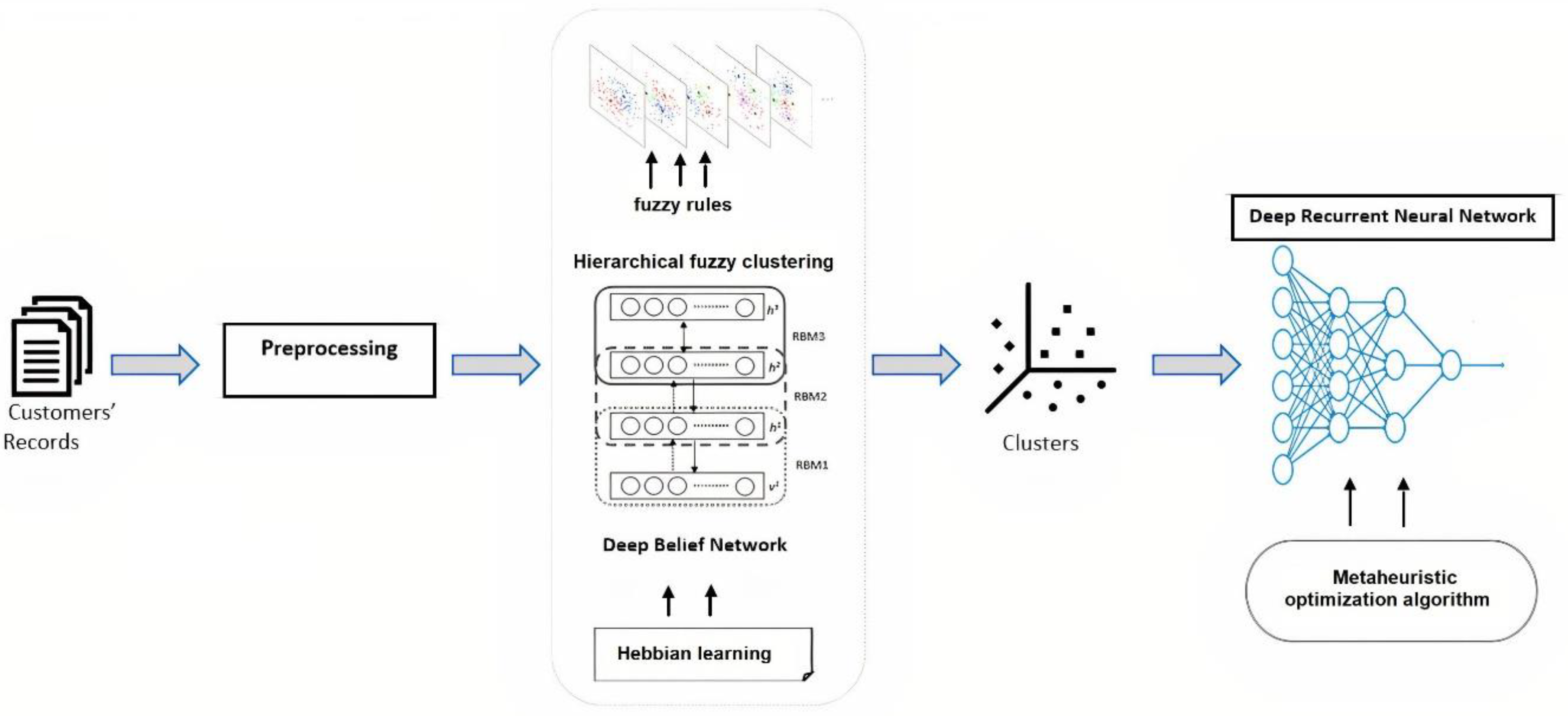
In this work, optimized clustering and deep learning techniques are utilized. Here, the deep belief neural network, Hebbian learning, and fuzzy clustering are combined to examine customer data on customers and their purchasing behaviors. According to similarity, customers are grouped, which helps identify their exact purchasing patterns. The clustered information is analyzed by an optimized deep recurrent neural network (ODRNN) to predict customer behavior. The network parameters are optimized according to a butterfly optimization algorithm (BOA) that minimizes the maximum error classification problem.

The major contributions of this work are as follows. The study (1) proposes a novel clustering approach on the basis of an optimized fuzzy deep belief network and compares it with different hard and fuzzy clustering approaches; (2) adopts an ODRNN that utilizes a BOA to predict customer behavior; (3) proposes a novel hybrid model that comprises two modules, namely a clustering module and a deep recurrent neural network module, and examines it on three benchmark customer datasets; (4) adopts four more advanced machine learning algorithms, specifically K-nearest neighbor, SVM, DNN, and CNN, to predict customer behavior and determine which method works best; and (5) investigates a number of hybrid models to solve customer behavior prediction problems and compare them with the proposed hybrid model. The rest of the paper is organized as follows: Section 2 elaborates on related work on customer behavior prediction. Section 3 and Section 4 explain the working process of the ODRNN-based customer behavior prediction approach. Section 5 explains the experimentation. Section 6 analyzes the efficiency of the introduced system. The results are then conclusively explained in Section 7.

2. Related Works

Customer behavior prediction has been conducted using several prediction methods and techniques. Singh et al. [11] developed a customer behavior pattern prediction approach by using K-means clustering. Customers’ purchasing patterns were analyzed, after which they were divided into different groups. The clustered information was given as an input to the inferior rule association technique. The a priori algorithm classifies customer patterns by covering enough purchasing patterns. This process improved prediction accuracy and resolved data availability issues effectively. Zare et al. [12] promoted client satisfaction by incorporating an advanced K-means clustering method. They assessed customer behavioral information by considering malevolent characteristics, criteria of purchase, and demographic details. Sampled characteristics were ranked according to behavioral features. Customers of the Hamkaran company were used to conduct the experiment, and the outcomes indicated that the advanced K-means strategy presented produced higher speed and accuracy than the K-means.

Zheng et al. [13] introduced an interpretable clustering-based churn identification process from customer transaction and demographic information. The collected details were processed by an inhomogeneous Poisson process that recognized customer churners. This process addresses running time and accuracy issues in the churn detection method.

A study by Yontar et al. [14] aimed to predict whether users of credit cards would pay off their debts. The support vector machine (SVM) algorithm showed that the potential perils of unpaid debt predicted were accurate and that relevant actions could be taken in due time. In their research, they used the information of 30,000 clients sourced from a major bank in Taiwan. The records contained client details, such as gender, level of education, credit amounts, age, marital status, invoice amount, early payment records, and credit card payments. The evaluation results indicated that SVM provides over 80% accuracy in predicting clients’ payment status in the subsequent month. Sahar and Sabbeh’s [15] work showed similarities; they evaluated the competence of various machine learning strategies used to solve problems related to customer relationships. Many analytic methods belonging to various learning groups were used in this analysis. These strategies included K-nearest neighbor (KNN), decision trees, SVM, naïve Bayesian, logistic regression, and multi-layer perceptions. They applied models to a telecommunication database containing 3333 records. Realized results indicated 94% accuracy for both multi-layer perception and SVM.

Kim et al. [16] used unstructured information and a convolutional neural network (CNN) to predict customer behaviors from online storefront information. Their system used a multi-layer perceptron network structure, which combined both structured and unstructured details to improve the learning process. The learning process deduced business problems related to frequent shoppers, churn, frequent refund shoppers, re-shoppers, and high-value shoppers. In addition, the network successfully minimized the deviation between actual and predicted customer behavior. The efficiency of the system was evaluated using Korean-based online storefront information, and the system ensured maximum prediction accuracy.

Ko et al. [17] incorporated a CNN to create a client retention identification system. They sourced customer information from transaction data, customer satisfaction scores, and purchasing rates. They also obtained conclusive information through the creation of data-driven questionnaires. Furthermore, they evaluated the collected data by using enterprise resource planning, which helps identify client loyalty and trust. This system classified customer retention by ensuring 84% accuracy. Additionally, Tariq et al. [18] recommended a CNN for creating a distributed model to predict customer churn. The main aim of the study was to monitor customer behavior with maximum accuracy. Their study used the Telco Customer Churn dataset, which was analyzed by data load, pre-processing, and convolutional layer. Along with this, the Apache Spark parallel framework was utilized to improve the data analysis process. The framework minimized validation loss by up to 0.004 and increased prediction rate accuracy by up to 95%.

Fridrich et al. [19] introduced a genetic algorithm in an artificial neural network (ANN) for optimizing hyper-parameters while recognizing customer churn. Their study aimed to maintain the robustness, trust, and reliability of the classification model. In their study, 10,000 customer lifetime values were collected and processed using neural functions to predict customer churn. During this process, network parameters were optimized according to genetic operators, such as set selection, mutation, and crossover. The optimal parameters helped reduce the deviation between predicted and actual customer behavior. To predict customer churn, Momin et al. [20] recommended a deep learning model with a multi-layer network. The proposed network uses several layers to examine customer details in an industry to predict churn data. IBM Telco’s customer churn dataset was then utilized for further analysis. This method uses a self-learning algorithm that reduces computation complexity. This implemented system ensured 82.83% accuracy and was compared to the decision tree, K-nearest neighbors (KNN), naive Bayes, and logistic networks. Lalwani et al. [21] proposed a methodology for prediction of customer churn. Feature selection was performed using a gravitational search algorithm. Various methods were examined in the prediction process, namely, logistic regression, naive Bayes, SVM, random forest, and decision trees. Additional boosting and ensemble mechanisms were applied and examined. The obtained results indicated that Adaboost and XGboost classifiers achieved the highest accuracies of 81.71% and 80.8%, respectively.

Edwine et al. [22] presented a method for identifying the risk of customer churn based on telecom datasets. The study compared advanced machine learning methods and applied optimization techniques. Hyper-parameter optimization algorithms such as grid search, random search, and genetic algorithms were applied to random forest, SVM, and KNN to predict customer churn. Experimental results showed that the random forest algorithm optimized by grid search achieved the highest numbers compared to the other models, with a maximum accuracy of 95%. Another study conducted by Arivazhagan and Sankara [23] predicted churn customers by employing a list of important attributes used to measure behavior before churning. The authors of this study focused on three sectors: e-commerce, banking, and telecom. An if–then rule was used to predict churn in addition to the identified attributes. A proposed Bayesian boosting with logistic regression (BLR) was applied to the dataset and compared with logistic regression. The obtained results indicated that the proposed BLR method gave accuracies of 94.42%, 95.54%, and 92.32% for e-commerce, bank, and telecom, respectively. Although the BLR handles bias, it requires a long processing time and needs to be improved.

Another study by Rabieyan et al. [24] forecasted client value through the application of an improved fuzzy neural network (IFNN). Fuzzy rules favored a continuous investigation of client purchasing details, demographics, and online participant data. Evaluation results comparing classical prediction methods and IFNN showed that the performance of the latter was better. They used root means square error (RMSE) as a measure of performance and their model recorded 0.061 of RMSE.

In their analysis, Sivasankar et al. [25] incorporated hybrid probabilistic possibility of fuzzy c-means clustering artificial neural networks (PPFCM-ANN) to predict client churn in a commercial enterprise. They gathered customer activity details from the business and applied the clustering technique. Afterward, they computed client relationships, preferences, and relevant probability values to form clusters. Furthermore, they investigated customer information by using a neural network predicting client churn according to similarity. Their model achieved good results among ten samples and accuracy reached 94.62%.

According to various customer behavior prediction models in the literature, machine learning techniques highly influence BI processes. However, some methods require considerable time to recognize behavior patterns, which leads to computational complexity. Other methods struggle with the maximum error classification problem. Existing prediction approaches have recorded low accuracy due to inadequate feature selection [21,26]. A feature selection mechanism can improve model performance and increase the predictive power of the applied algorithm. Applying feature selection before data processing leads to more accurate results. Additionally, most recent deep neural network (DNN) models used in customer behavior classification suffer from overfitting, and a prevention technique is not taken into consideration [21]. Furthermore, a number of studies have concluded that the most accurate results are given by hybrid models rather than single models [27]. However, most customer behavior prediction models are singular. Moreover, most studies in the field examined their models on private datasets extracted from local businesses. There is a lack of studies using benchmark datasets. Using benchmark datasets organizes researchers around specific research areas and acts as a measure of performance. All these issues are addressed in this study.

In short, there is still room for the improvement of behavior prediction models. This requires optimized and hybrid techniques to analyze customer behavior patterns with maximum accuracy. Combining modalities rather than using a single modality can positively affect the prediction of customer behavioral patterns. The deep learning model has been demonstrated to be a promising solution, especially when combined with the right approaches. As such, clustering and optimized deep learning methods are utilized in this work to improve the overall customer behavior prediction process. The working process of the system proposed in this paper is detailed in the following sections.

3. Enhanced Fuzzy Clustering Algorithm

To improve the clustering process and achieve a minimum error rate and an optimum clustering scheme, deep belief neural networks and the Hebbian learning approach were combined with hierarchical fuzzy clustering (HFC). Each of these techniques involves a specific learning concept and processing function that clusters customers more efficiently based on relevant data. An inadequate learning pattern causes a maximum error rate classification problem that directly impacts the prediction rate. Hence, optimized clustering techniques should be integrated to improve system performance. The overall customer behavior prediction model is illustrated in Figure 1.

3.1. Hierarchical Fuzzy Clustering

This section discusses the first stage of the system, HFC. A cluster is a group of similar objects that are similar between them and are dissimilar to objects in other clusters. Clustering involves finding a structure in a collection of unlabeled data [28]. HFC is an unsupervised clustering technique used to build a cluster by examining data. The main intention of this HFC is to group similar information, and each cluster differs from others. Similarity is computed according to a distance matrix, which helps predict the two clusters that are closest to each other and merge the similar information in the two clusters. According to the distance measure the hierarchical relationship is computed. During the clustering process, fuzzy rules are set to determine the conditions for grouping.

In this work, the clustering process determined the differences between the non-numeric information based on Equation (1), which examines the relationship between the data.

$${\mathit{lev}}_{\mathit{a},\mathit{b}}\left(\mathit{i},\mathit{j}\right)=\{\begin{array}{c}\mathbf{max}\left(\mathit{i},\mathit{j}\right) \mathbf{if} \mathbf{min}\left(\mathit{i},\mathit{j}\right)=0,\\ \mathbf{min}\{\begin{array}{c}{\mathit{lev}}_{\mathit{a},\mathit{b}}\left(\mathit{i}-1,\mathit{j}\right)+1\\ {\mathit{lev}}_{\mathit{a},\mathit{b}}\left(\mathit{i},\mathit{j}-1\right)+1\\ {\mathit{lev}}_{\mathit{a},\mathit{b}}\left(\mathit{i}-1,\mathit{j}-1\right){+1}_{\left({\mathit{a}}_{\mathit{i}}\ne {\mathit{b}}_{\mathit{j}}\right)}\end{array} \mathbf{otherwise}\end{array}$$

(1)

In Equation (1), data distance is denoted as ${\mathit{lev}}_{\mathit{a},\mathit{b}}\left(\mathit{i},\mathit{j}\right)$, which is estimated between the a and b strings. The non-numeric data distance ${\mathit{lev}}_{\mathit{a},\mathit{b}}\left(\mathit{i},\mathit{j}\right)$ is computed between two strings, $\mathit{a} \mathrm{and} \mathit{b}$. Here, the length of the string is represented as $\left|\mathit{a}\right|$ and $\left|\mathit{b}\right|$, which helps compute the distance between two strings. Here, the membership value that is the indicator function $1_{\left({\mathit{a}}_{\mathit{i}}\ne {\mathit{b}}_{\mathit{j}}\right)}$ is utilized to compute the distance value of ${\mathit{a}}_{\mathit{i}}$ and ${\mathit{b}}_{\mathit{j}}$. If the values are equal, then the value assigned is one, or zero otherwise. The first character in a is represented as $\mathit{i}$, while the b string’s first character is denoted as j, and the distance between these characters is denoted as ${\mathit{lev}}_{\mathit{a},\mathit{b}}\left(\mathit{i},\mathit{j}\right)$. Then, the cluster linkage is estimated using Equation (2).

$$\mathbf{linkage} \mathbf{cluster}=\mathbf{max}\left\{\mathit{d}\left(\mathit{a},\mathit{b}\right):\mathit{a}\in \mathit{A},\mathit{b}\in \mathit{B}\right\}$$

(2)

The computed distance and linkage values in the data are investigated, and similar information is grouped. During this process, the fuzzy approach is applied to compute the cluster center. This allocation process uses the membership function, set theory, and fuzzy rules to identify a specific class. Fuzzy logic is utilized to form soft clustering, which has a value of [0, 1]. The fuzzy membership values determine whether particular data belongs to a specific set or not. The exactness of the data is computed using the fuzzy membership value. Therefore, here, the fuzzy rules and logics are incorporated with the HFC process. Most of the fuzzy applications belong to linguistic variables such as Medium, Low, and High, which are used to allocate the data to specific classes. The linguistic variables are defined via fuzzy set by performing the fuzzification process, which is performed by applying the membership function. Considering X, the customer information belonging to the specific class c, the respective membership value is estimated using Equation (3).

$$\begin{array}{c}\{{\mathsf{\mu }}_{\mathit{j}}:\mathit{X}\to \left[0,1\right], \mathit{j}=1,\dots .\mathit{c} \\ {\displaystyle {\displaystyle \sum }_{\mathit{j}=1}^{\mathit{c}}}{\mathsf{\mu }}_{\mathit{j}}\left({\mathit{x}}_{\mathit{i}}\right)=1, \mathit{i}=1,2,\dots \mathit{n}\\ 0<{\displaystyle {\displaystyle \sum }_{\mathit{i}=1}^{\mathit{n}}}{\mathsf{\mu }}_{\mathit{j}}\left({\mathit{x}}_{\mathit{i}}\right)<\mathit{n} \mathit{j}=1,2,\dots .\mathit{c}\end{array}\}$$

(3)

According to Equation (3), the membership value of each user is estimated from the distance value and the cluster center. The membership values belonging to 0,1 and the data point membership values are computed within cluster c. Therefore, the membership value ${\mathsf{\mu }}_{\mathit{j}}\left({\mathit{x}}_{\mathit{i}}\right)$ is computed and the range comes under $0<{\displaystyle \sum }_{\mathit{i}=1}^{\mathit{n}}{\mathsf{\mu }}_{\mathit{j}}\left({\mathit{x}}_{\mathit{i}}\right)<\mathit{n}$. As mentioned earlier, the cluster center should be predicted to reduce the standard loss function (SLF) and improve overall clustering accuracy. The SLF value is obtained from Equation (4).

$$\mathbf{SLF}={\displaystyle \sum }_{\mathit{k}=1}^{\mathit{c}}{\displaystyle \sum }_{\mathit{i}=1}^{\mathit{n}}{\left[{\mathsf{\mu }}_{\mathit{k}}{(\mathit{x}}_{\mathit{i}})\right]}^{\mathit{m}}\Vert {\mathit{x}}_{\mathit{i}}{-\mathit{c}}_{\mathit{k}}\Vert {}^2$$

(4)

The loss function value is computed from the cluster center ${\mathit{c}}_{\mathit{k} }$, which is obtained from the ith membership function defined in Equations (5) and (6). The loss function is estimated along with the x_i membership value ${\mathsf{\mu }}_{\mathit{k}}{(\mathit{x}}_{\mathit{i}})$ and the difference between the input and cluster distance measures $\Vert {\mathit{x}}_{\mathit{i}}{-\mathit{c}}_{\mathit{k}}\Vert {}^2$.

$${\mathit{c}}_{\mathit{k}}=\frac{{{\displaystyle \sum }}_{\mathit{i}}{\left[{\mathsf{\mu }}_{\mathit{k}}{(\mathit{x}}_{\mathit{i}})\right]}^{\mathit{m}}{\mathit{x}}_{\mathit{i}}}{{{\displaystyle \sum }}_{\mathit{i}}{\left[{\mathsf{\mu }}_{\mathit{k}}{(\mathit{x}}_{\mathit{i}})\right]}^{\mathit{m}}}$$

(5)

$${\mathsf{\mu }}_{\mathit{k}}\left({\mathit{x}}_{\mathit{i}}\right)=\frac{{\left({1/\mathit{d}}_{\mathit{ki}}\right)}^{1/(\mathit{m}-1)}}{{{\displaystyle \sum }}_{\mathit{k}=1}^{\mathit{c}}{\left({1/\mathit{d}}_{\mathit{ki}}\right)}^{1/(\mathit{m}-1)}}$$

(6)

The cluster center ${\mathit{c}}_{\mathit{k}}$ is computed from the membership value ${\mathsf{\mu }}_{\mathit{k}}$ and respective sample observation ${\mathit{x}}_{\mathit{i}}$. In the membership value, the distance between the $\mathit{i}\mathrm{th}$ observation in the $\mathit{k}$ cluster is defined as ${\mathit{d}}_{\mathit{ki}}$. According to the cluster center, the membership function and linkage clusters of customers with similar purchasing patterns are identified and grouped.

3.2. Deep Belief and Hebbian Learning Rule Clustering

HFC was utilized to investigate customer data according to fuzzy rules. Here, the deep belief network (DBN) and the Hebbian learning rule were combined with HFC to perform the whole clustering process and further improve the customer prediction rate. The main intention of this study was to reduce computation time and increase the accuracy of the prediction rate.

3.2.1. Deep Belief Network

Deep learning has an impeccable effect on the unsupervised learning of representations. The DBN is a well-known category of DNNs, which is characterized by a multi-layered graphical model with directed and undirected edges. Multiple layers are interconnected, but the hidden units in each layer are separated from each other. One advantage of this deep architecture is that each successive layer discovers more complex features unseen by the preceding layer. As a deep architecture, the DBN is founded on multiple layers of stacked, restricted Boltzmann machines (RBMs). An RBM is a two-layer network with one visible layer and one hidden layer, with no connections between the nodes in a single layer [29].

The stacked RBM layers form a network with the capacity to discover regularities and invariances in raw data. An RBM in one layer feeds the RBM in the succeeding layer. In this way, high-level dependencies are progressively extracted and refined [30]. A DBN involves two stages: pre-training and fine-tuning. In the pre-training stage, each of the stacked RBMs is trained with the visible units v ∈ {0, 1} representing the input data, and the set of hidden units h ∈ {0, 1} refers to the feature detector. Training occurs through a bottom-up process, starting with the RBM at the lower level, which receives DBN inputs. The training progresses upward until the top-most layer, which is the DBN output, is reached and trained. The learning process is relatively efficient and largely unsupervised; as such, it fits the features of the samples. Consequently, the output of a hidden layer in one RBM can be used as the input for a visible layer in another RBM [29,31]. This process allows for the extraction of more features from a dataset.

The working process of DBN clustering (DBNC) is illustrated in Figure 2a,b. This process improves the accuracy of the customer prediction rate.

In the pre-training step, the network has RBM-based hidden variables that have connections such as input to hidden or hidden to hidden [26]. The variable in the network has an energy model with a separate state, which is more useful in forming the cluster. The visible and hidden nodes’ energy state levels are estimated using Equation (7).

$$\mathit{E}\left(\mathit{v},\mathit{h},\mathsf{\theta }\right)=-{\displaystyle \sum }_{\mathit{i}\in \mathit{visible}}{\mathit{a}}_{\mathit{i}}{\mathit{v}}_{\mathit{i}}-{\displaystyle \sum }_{\mathit{j}\in \mathit{hidden}}{\mathit{b}}_{\mathit{j}}{\mathit{h}}_{\mathit{j}}-{\displaystyle \sum }_{\mathit{i},\mathit{j}}{\mathit{v}}_{\mathit{i}}{\mathit{h}}_{\mathit{j}}{\mathit{w}}_{\mathit{i},\mathit{j}}$$

(7)

In Equation (7), the model parameter is defined as $\mathsf{\theta }=\left\{\mathit{w},\mathit{a},\mathit{b}\right\}$, the weight between i (visible unit) and j (hidden unit) is denoted as ${\mathit{w}}_{\mathit{i},\mathit{j}}$, and biases are represented as ${\mathit{a}}_{\mathit{i}}$ and ${\mathit{b}}_{\mathit{j}}$. The computed state value helps assign the probability value to every visible and hidden vector pair. The probability assignment is performed using Equation (8).

$$\mathit{P}\left(\mathit{v},\mathit{h}\right)=\frac{1}{\mathit{Z}}{\mathit{e}}^{-\mathit{E}\left(\mathit{v},\mathit{h},\mathsf{\theta }\right)}$$

(8)

The Z value in Equation (8) is computed as $\mathit{Z}={\displaystyle \sum }_{\mathit{v},\mathit{h}}{\mathit{e}}^{-\mathit{E}\left(\mathit{v},\mathit{h},\mathsf{\theta }\right)}$. In other words, the visible–hidden feature vector summation is utilized to calculate the Z value.

Then, the data probability value is estimated over hidden units Equation (9).

$$\mathit{P}\left(\mathit{v}\right)=\frac{1}{\mathit{Z}}{\displaystyle \sum }_{\mathit{h}}{\mathit{e}}^{-\mathit{E}\left(\mathit{v},\mathit{h},\mathsf{\theta }\right)}$$

(9)

The probability value is estimated from visible and hidden node exponential value. Along with these nodes, network parameters, namely weight and bias values, are included. During the visible–hidden node and data probability computation process, the RBM weight and bias value should be monitored continuously. Suppose that the network requires a high deviation; the RBM has a high energy value while processing the inputs. Therefore, the network parameters should be updated to reduce the input vector energy consumption. The network must be trained to predict new customer information with minimal computational complexity. Therefore, the log-type probability value is utilized to train the features. It is estimated as follows:

$$\frac{\partial \mathbf{log}\mathit{P}\left(\mathit{v}\right)}{\partial {\mathit{w}}_{\mathit{ij}}}{=\langle \mathit{v}}_{\mathit{i}}{\mathit{h}}_{\mathit{j}}\rangle {}_{\mathit{Data}}{-\langle \mathit{v}}_{\mathit{i}}{,\mathit{h}}_{\mathit{j}}\rangle {}_{\mathit{model}}$$

(10)

Here, the contrastive divergence learning function is applied to train the information, and the network parameters are updated using Equation (11).

$$\Delta {\mathit{w}}_{\mathit{ij}}=\mathit{ϵ}\left(\langle {\mathit{v}}_{\mathit{i}}{\mathit{h}}_{\mathit{j}}\langle {}_{\mathit{Data}}{-\langle \mathit{v}}_{\mathit{i}}{,\mathit{h}}_{\mathit{j}}\rangle {}_{\mathit{model}}\right)$$

(11)

The weight value is updated from the deviation between the visible–hidden data pair value and visible–hidden model pair value along with the learning rate $\mathit{ϵ}$.

The next part utilizes the deep auto encoder to unroll the RBM with pre-trained weight values. Here, multi-layer functionalities are used to reconstruct one visible input to another representation, which is defined in Equation (12).

$$\mathit{RE}=-\mathbf{log}\mathit{P}\left(\mathit{X}\left|\mathit{R}\right(\mathit{X},\mathit{W})\right)$$

(12)

The $\left(\mathit{X}\left|\mathit{R}\right(\mathit{X},\mathit{W})\right)$ logarithmic values are computed to obtain the Gaussian loss function, and the probability value is defined to obtain the squared error value.

$$-\mathbf{log}\left(\mathit{X}|\mathit{R}\left(\mathit{X},\mathit{W}\right)\right)=-{\displaystyle \sum }_{\mathit{i}}{\mathit{x}}_{\mathit{i}}{\mathbf{log}\mathit{f}}_{\mathit{i}}\mathit{R}\left(\mathit{X},\mathit{W}\right)-{\displaystyle \sum }_{\mathit{i}}\left({1-\mathit{x}}_{\mathit{i}}\right)\mathbf{log}\left({1-\mathit{f}}_{\mathit{i}}\mathit{R}\left(\mathit{X},\mathit{W}\right)\right)$$

(13)

The inputs from the layers are reconstructed and defined as ${\mathit{f}}_{\mathit{i}}\mathit{R}\left(\mathit{X},\mathit{W}\right)$. In addition, backpropagation and gradient methods are used to reduce the loss function, which helps to resolve the maximum error classification problem.

After performing a high-level learning representation, fuzzy clustering is applied to cluster customers according to their behavior. The clustering process helps in understanding complex customer purchasing behaviors. During clustering, the cluster center ${\mathit{c}}_0$ membership matrix is ${\mathsf{\mu }}_0$ and the weight value W is initialized and regularized continuously. The regularization of the clustering parameter in Equation (14) minimizes the error rate.

$$\mathit{f}=\mathit{e}\ast (-{\displaystyle \sum }_{\mathit{i}}{\mathit{x}}_{\mathit{i}}{\mathbf{log}\mathit{f}}_{\mathit{i}}\mathit{R}\left({\mathit{x}}_{\mathit{i}},\mathit{W}\right))-{\displaystyle \sum }_{\mathit{i}}\left({1-\mathit{x}}_{\mathit{i}}\right)\mathbf{log}\left({1-\mathit{f}}_{\mathit{i}}\mathit{R}\left({\mathit{x}}_{\mathit{i}}{,\mathit{W}}_{\mathit{i}}\right)\right)+\left(1-\mathit{e}\right)\ast {\displaystyle \sum }_{\mathit{i}=1}^{\mathit{N}}{\displaystyle \sum }_{\mathit{j}=1}^{\mathit{C}}\sqrt{{(\mathit{R}\left({\mathit{x}}_{\mathit{i}}{,\mathit{W}}_{\mathit{i}}\right){-\mathit{c}}_{\mathit{j}})}^2}$$

(14)

For every customer input ${\mathit{f}}_{\mathit{i}}\mathit{R}\left({\mathit{x}}_{\mathit{i}},\mathit{W}\right)$, clusters are formed by investigating neural network parameters, activation functions, and loss functions. The computed clustered output is regularized using regulation factor $\mathit{e}$. Then, the loss function is updated using Equation (15).

$$\mathit{f}=\mathit{e}\ast (-{\displaystyle \sum }_{\mathit{i}}{\mathit{x}}_{\mathit{i}}{\mathbf{log}\mathit{f}}_{\mathit{i}}\mathit{R}\left({\mathit{x}}_{\mathit{i}},\mathit{W}\right))-{\displaystyle \sum }_{\mathit{i}}\left({1-\mathit{x}}_{\mathit{i}}\right)\mathbf{log}\left({1-\mathit{f}}_{\mathit{i}}\mathit{R}\left({\mathit{x}}_{\mathit{i}}{,\mathit{W}}_{\mathit{i}}\right)\right)+1/2\left(1-\mathit{e}\right)\ast {\displaystyle \sum }_{\mathit{i}=1}^{\mathit{N}}{\displaystyle \sum }_{\mathit{j}=1}^{\mathit{C}}\sqrt{{(\mathit{R}\left({\mathit{x}}_{\mathit{i}}{,\mathit{W}}_{\mathit{i}}\right){-\mathit{c}}_{\mathit{j}})}^2}$$

(15)

Assume the cluster center has known parameter weight value $\mathit{W}$, the derivation of the loss function value is computed with respect to the weight parameter, and the compound function is defined as ${\mathit{f}}_{\mathit{i}}\mathit{R}\left({\mathit{x}}_{\mathit{i}},\mathit{W}\right)$. The compound function is computed with respect to the input X and $\mathit{R}\left({\mathit{x}}_{\mathit{i}},\mathit{W}\right)$ is defined as the changing compound function, which reduces the error rate value. Then, the loss function changes are defined using Equation (13). The minimum loss function indicates that the clustering algorithm effectively groups similar data. Then, the pre-trained cluster values are effectively examined in the fuzzy clustering process to improve the overall prediction rate.

At the time of clustering, the network uses 500, 300, and 100 neurons in three layers that process the inputs. Then, clusters are formed randomly by applying 0.05 and 0.1 learning rates. This process was performed with 32 batch sizes and, for 50 iterations; the network produced a 0 to 1 loss function on maximum epochs. At the time of computation, if the loss function gives 0, weight tuning is fully taken on sum inner-cluster distance. Whereas if the loss function gives 1, weight tuning is fully taken on auto-encoder. MSE is the basis for selecting the best value among all the tested ones, where the lowest MSE is considered best. It was found that 0.5 gave the best results. The maximum iterations to form pre-training and fine-tuning is 50 iterations. During this process, inputs are continually analyzed in the pre-trained phase, and the decoding stage reconstructs the information to minimize the error value. The hyper-parameters of the constructed DBN are illustrated in

Table 1. Hyper-parameter setting of DBN.

Hyper-Parameter	Value
Learning rate	0.0005
Number of hidden layers	3
Number of nodes in each layer	500, 300, 100
Initial momentum	0.5
Momentum	0.9
Delay in momentum	3
Batch size	256
Epochs	200
Gap delay	10
Gap stop delay	2

.

3.2.2. Hebbian Learning Rule

Unsupervised learning involves various principles and algorithms. Among them is the Hebbian principle, which states that human learning involves the strengthening of the connections linking two neurons as a result of simultaneous activation [32]. Hebbian learning (HBL) comes from a physiological learning technique, the foundation of which is the reinforcement of linkages between neurons. The HBL algorithm enhances the process of learning within a neural network. This learning concept involves certain assumptions, one of which is that the simultaneous activation and deactivation of two neurons may result in an increase in the weight of the neurons, whereas reversing the occurrence of the operation leads to a decrease in the neurons’ weight [33]. This is defined as a synaptic weight adjustment technique for artificial neurons. Hebb’s principle states that the weight of the connection between two neurons increases in cases of simultaneous activation and decreases in cases of separate activation. This learning rule is applied to neural networks, which learn the computational process from existing conditions to enhance overall classification performance [34].

During the clustering process, a set of Hebbian learning rules is applied to estimate the relationship between the inputs. The learning rules solves the categorization and classification problems within large data analysis. The utilized Hebbian rules are defined in Equation (16).

$${\mathit{w}}_{\mathit{ij}}\left[\mathit{n}+1\right]{=\mathit{w}}_{\mathit{ij}}\left[\mathit{n}\right]{+\mathsf{\eta }\mathit{x}}_{\mathit{i}}\left[\mathit{n}\right]{\mathit{x}}_{\mathit{j}}\left[\mathit{n}\right]$$

(16)

The HBL process uses the learning rate coefficient $\mathsf{\eta }$ to estimate each input i and the jth element. Here, two neurons are deactivated and activated at the same time. This learning process uses a weight value that is proportional to the learning time. The Hebbian rule is utilized in the weight updating process, which is conducted using Equation (17).

$${\mathit{w}}_{\mathit{ij}}{=\mathit{x}}_{\mathit{i}}{\ast \mathit{x}}_{\mathit{j}}$$

(17)

This learning improves the overall network weight updating process and clustering efficiency. The DBN-HBL-based clustering is illustrated in Algorithm 1.

Algorithm 1 DBN-HBL-based Clustering

Input:x input, $\mathit{\eta }$ learning parameter, i,j is the input, hidden layer X, cluster center c, membership function $\mathit{\mu }$, maximum iteration, maximum epoch (me),  e, r, and ${\mathit{w}}_{\mathit{i}\mathit{j}}\left[\mathit{n}\right]$. Output: final membership matrix $\mathit{\mu }$, final cluster c, distance matrix D, W For k = 1 to me do     Encode with w (0) and learning representation R (k)   Form cluster with R   Generate new cluster $\mathit{\mu }$ (k)     Calculate D   Perform decoding and backpropagation to reduce the loss function  Update weight value from (w (k − 1) to w (k)) according to the Hebbian rule.           ${\mathit{w}}_{\mathit{i}\mathit{j}}\left[\mathit{n}+1\right]={\mathit{w}}_{\mathit{i}\mathit{j}}\left[\mathit{n}\right]+\mathit{\eta }{\mathit{x}}_{\mathit{i}}\left[\mathit{n}\right]{\mathit{x}}_{\mathit{j}}\left[\mathit{n}\right]$ ${\mathit{w}}_{\mathit{i}\mathit{j}}={\mathit{x}}_{\mathit{i}}\ast {\mathit{x}}_{\mathit{j}}$

The HBL algorithm is used to update network parameters such as weight and bias. All processing information is stored between the neuron connections in the form of weights. The weights must be changed continuously to obtain the appropriate output value. The changed weight values are proportional to the neurons’ activation values. The neuron weight values are updated according to Equations (16) and (17), which is performed repeatedly to increase the overall network performance. Here, the weight updating process is applied while searching the inputs in the searching process. This learning rule is applied between the neurons’ connections because it is used to minimize the loss values. Once the clusters are formed, they are processed by applying deep recurrent neural networks to predict customer behavior, which is discussed in the next section. Here, the MATLAB tool is used to implement the process. The implementation tool itself has the neural network toolbox and fuzzy logic toolbox. These toolboxes support the various functions and libraries that support this clustering process.

4. Customer Behavior Prediction

Following clustering formalization, deep learning is applied in stage two, which decreases the duration of learning and reduces tolerance from the overfitting risk [35,36].

Deep learning strategies can learn several representation levels from raw data inputs without involving rules or expert knowledge. A recurrent neural network (RNN) is a feed-forward neural network with an internal memory that retains the processed input [37]. The memory-based network aids in improving prediction time while investigating new customer details. At this stage, the architecture is a DNN that predicts customer behavior through the use of multiple layers exhibiting temporal feedback loops in every layer, or a DRNN. New information moves up the hierarchy, adding temporal context to every layer in every network update. The DRNN incorporates the DNN concept with the RNN, where every hierarchical layer is an RNN (Figure 3). Every layer that follows receives the hidden state of the former layer as a series of input times. The automatic assembling of RNNs generates various time scales at different levels, thus producing a temporal hierarchy [37].

The clustered customer information is given as inputs in this stage, and customer behavior is predicted by applying the ODRNN. The network uses the memory state that saves every processing input detail. The network consists of an input layer, a hidden layer, and an output layer. In every layer, the output is computed to obtain customer behavior. The hidden layer processes the inputs, and the output is obtained using Equation (18).

$${\mathit{h}}_{\mathit{t}}{=\mathsf{\sigma }}_{\mathit{h}}\left({\mathit{W}}_{\mathit{h}}{\mathit{x}}_{\mathit{t}}{+\mathit{U}}_{\mathit{h}}{\mathit{h}}_{\mathit{t}-1}{+\mathit{b}}_{\mathit{h}}\right)$$

(18)

Here, the hidden layer output ${\mathit{h}}_{\mathit{t}}$ is computed from the processing of inputs, the network parameter U, weight W, bias b, and hidden vector ${\mathit{h}}_{\mathit{t}-1}$. The estimated output is then passed to the next layer to obtain the overall output ${\mathit{y}}_{\mathit{t}}{=\mathsf{\sigma }}_{\mathit{y}}\left({\mathit{W}}_{\mathit{y}}{\mathit{h}}_{\mathit{t}}{+\mathit{b}}_{\mathit{y}}\right)$. The output of the network ${\mathit{y}}_{\mathit{t}}$ is obtained from the output layer activation function ${\mathsf{\sigma }}_{\mathit{y}}$ applied to the output of the hidden layer, the weight multiplication process, and the output layer bias value ${\mathit{b}}_{\mathit{y}}$. During the computation, the sigmoid activation function $\mathsf{\sigma }=\frac{1}{{1+\mathsf{\sigma }}^{-\mathit{x}}}$ is utilized to get the output (0 and 1 or 1 and −1). If the output returns a 1, then the customer is considered willing to purchase the product in the future; otherwise (0 or −1), they are not interested in purchasing the product. Additional binary classifications related to customer behavior were studied, including the attractiveness of the customer and product upselling predictions.

This computation is more effective because the clustering process also utilizes the probability value for visible and hidden vectors. This selects the most similar and relevant information; likewise, a recurrent network also uses the $\mathit{P}\left({\mathit{o}}^{\mathit{u}}{|\mathit{x}}_1^{\mathit{u}}{,\dots \dots \mathit{x}}_{\mathit{T}}^{\mathit{u}}\right)$ value for every order of customer. The probability value is computed from the customer’s previous purchasing orders to obtain user preferences; therefore, it minimizes the binary classification problem. Parameters tuning effects on improving the performance, such as increasing the number of neurons, batch size, and number of epochs. Hyper-parameter tuning can be performed with multiple trials until the best outcome is found. Nevertheless, the appropriate number of epochs can be selected by an early stopping mechanism, which can stop the training process after a number of epochs when finding the best validation numbers. Furthermore, the system should concentrate on the maximization error rate classification issue. This was resolved by optimizing the network parameters; the optimization was conducted by applying the BOA. The BOA resolves convergence issues by using the objective function, which also diminishes gradient issues. Here, butterfly characteristics are utilized to achieve the objective of the work. Stimulus variance intensity (SI) and fragrance $\mathit{fr}$ characteristics are used to identify the relationship between the network parameters. The SI of the network parameter is related to the encoded objective function. From the SI value, the fragrance is estimated using Equation (19).

$${\mathit{fr}=\mathit{smSI}}^{\mathit{e}}$$

(19)

The fragrance of the network parameter is estimated according to the sensory modality $\mathit{sm}$ and dependent modality exponent $\mathit{e}$ values. The range of $\mathit{sm}$ and $\mathit{e}$ values varies from (0,1). In the initialization of these parameters, the weight updating process is performed in global and local searching processes.

$${\mathit{b}}_{\mathit{u}}^{\mathit{it}+1}{=\mathit{b}}_{\mathit{u}}^{\mathit{it}}+\left({\mathit{rnd}}^2{\ast \mathit{h}}^{\ast }{-\mathit{b}}_{\mathit{u}}^{\mathit{it}}\right){\ast \mathit{fr}}_{\mathit{u}}$$

(20)

According to the above solution, the butterfly moves in the search space, and the global solutions are obtained from ${\mathit{b}}_{\mathit{u}}$ in the $\mathit{u}$-th iterations. From the computation, the best solution ${\mathit{h}}^{\ast }$ is obtained using Equation (21).

$${\mathit{b}}_{\mathit{u}}^{\mathit{it}+1}{=\mathit{b}}_{\mathit{u}}^{\mathit{it}}+\left({\mathit{rnd}}^2{\ast \mathit{b}}_{\mathit{v}}^{\mathit{it}}{-\mathit{b}}_{\mathit{w}}^{\mathit{it}}\right){\ast \mathit{fr}}_{\mathit{u}}$$

(21)

Equation (19) denotes the local search phase of the BOA, where ${\mathit{b}}_{\mathit{v}}^{\mathit{it}}$ and ${\mathit{b}}_{\mathit{w}}^{\mathit{it}}$ are the $\mathit{v}$-th and $\mathit{w}$-th butterflies from the solution space. If ${\mathit{b}}_{\mathit{v}}^{\mathit{it}}$ and ${\mathit{b}}_{\mathit{w}}^{\mathit{it}}$ butterflies belong to the same swarm and $\mathit{rnd}$ is a random number between the range [0, 1], then Equation (16) becomes a local random walk. A switch probability $\mathit{sp}$ in BOA helps switch between common global and local searches. This iteration is continued until the stopping criteria are matched. According to the optimization algorithm, the deep recurrent network is trained, and the respective parameters are updated to minimize loss values while predicting customer behavior.

5. Experimentation

The datasets utilized in the research were the KDD Cup 2009 orange small dataset [38], IBM Telco Customer Churn dataset [39], and IBM Watson Marketing Customer Value Dataset information [40]. The collected data consisted of several unwanted, inconsistent, and missing values that reduced the performance of the behavior prediction model. Therefore, missing values were replaced by computing mean values, which successfully removed outliers from the data ets. This pre-processing step reduced unwanted data and noise that might affect prediction accuracy.

The introduced DBN-HBL clustering and ODRNN-based customer behavior prediction were implemented using the MATLAB tool. Here, the neural network used the pre-training and fine-tuning steps to observe the customer information. For every customer order, probability values were computed to determine user preferences. The formed clusters were fed to the BOA-based deep RNN (BOA-DRNN). The network used a 0.05 learning rate, and a batch size of 512 was utilized to classify customer purchasing behavior. The K-fold cross-validation method was chosen as the base validation for comparison and tuning. The system evaluated using different cross-validation methods: test/train splitting, 5-fold cross-validation, and 10-fold cross-validation, and they showed varying results, with 10-fold being the best. The models were therefore trained and validated using 10-fold cross-validation. Initially, a dataset was divided into ten folds to evaluate the effectiveness of the system. The first fold was treated as the test model and the remaining models were considered as the training model. This process was repeated until k = 10. The continuous checking of the data minimized the error rate. In each iteration, grid-search-based hyper-parameter tuning was applied until the training and validation errors were steadied. This process helped solve hyper-parameter overfitting.

The proposed approach was examined and evaluated based on three sets of experiments. They are all explained in the following section.

6. Evaluation and Discussion

6.1. Clustering

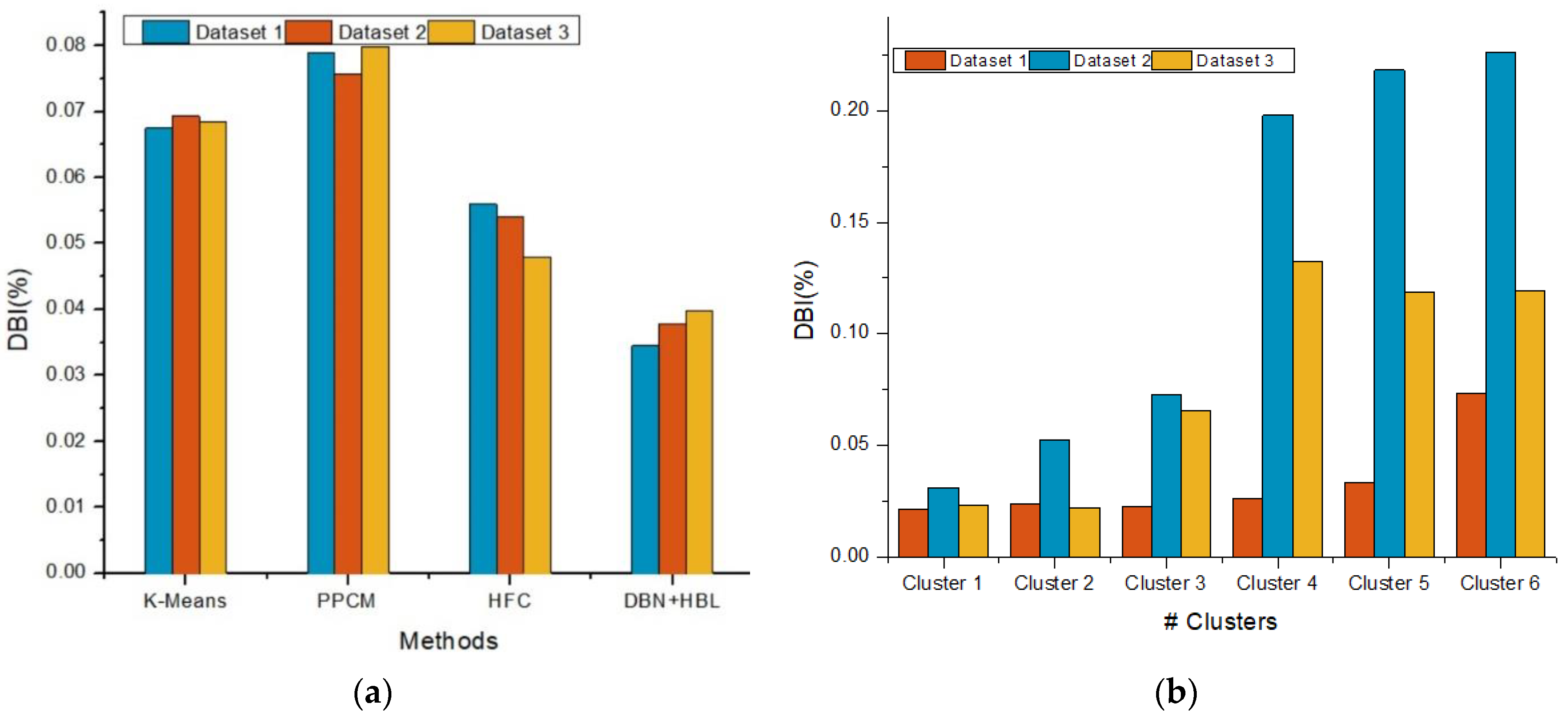
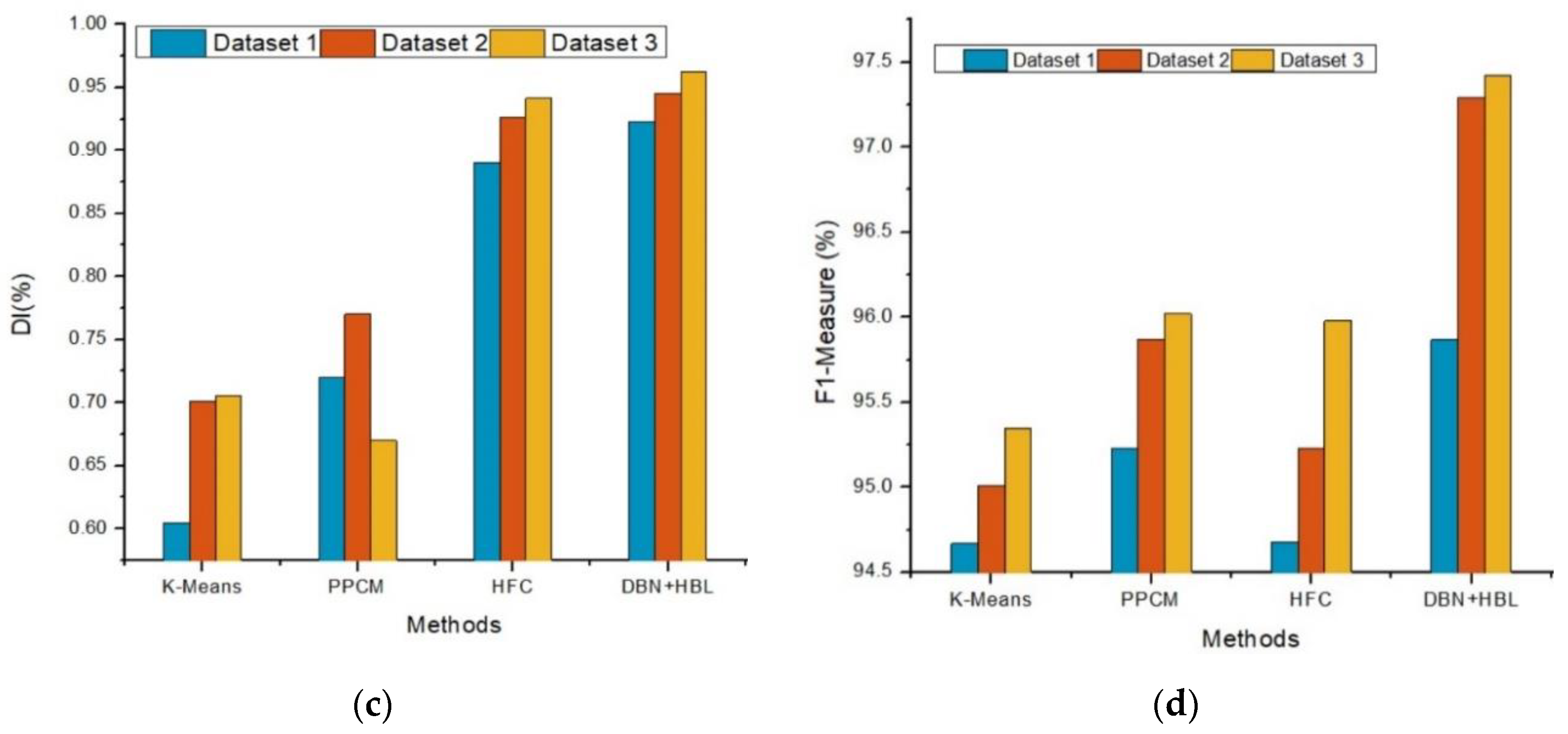
In the clustering stage, the results were compared to other clustering methods used in customer behavior prediction, such as K-means, and related forms of fuzzy clustering, such as HFC and probabilistic possibilistic fuzzy c-means clustering (PPFCM) [25]. Figure 3, Figure 4 and Figure 5 show the clustering evaluation results of the improved clustering approach compared to others based on the Davies–Bouldin index (DBI), Dunn index (DuI), silhouette coefficient (SC), Rand index (RI), Dice index (DI), and F-measure.

The DBN-HBL approach achieves a low DBI rate because the clustering approach uses the network structure in two phases: pre-training and fine-tuning. These phases are more helpful in predicting the similarities between customer information. In addition, regularized input values during clustering improve the overall cluster process.

Moreover, the DBN-HBL method examines the number of clusters and cluster centers using fuzzy rules and membership values. The effective selection of a cluster center improves the overall effectiveness of the clustering process. Therefore, the system predicts the similarity between customer features with a low DBI value. Here, before clustering, the HBL rule is applied to learn the customer features, and the clusters are formed accordingly. The learning process helps form a more accurate cluster compared to other methods.

Figure 4 illustrates DuI analysis of the DBN-HBL method. DuI is used to evaluate how effectively the method computes similarity value and how effectively the clusters are formed. The DBN-HBL approach attained a higher DuI rate because the clustering centers and fuzzy rules are applied according to the learning process. During this process, visible and hidden layer pair values $\mathit{E}\left(\mathit{v},\mathit{h},\mathsf{\theta }\right)=-{\displaystyle \sum }_{\mathit{i}\in \mathit{visible}}{\mathit{a}}_{\mathit{i}}{\mathit{v}}_{\mathit{i}}-{\displaystyle \sum }_{\mathit{j}\in \mathit{hidden}}{\mathit{b}}_{\mathit{j}}{\mathit{h}}_{\mathit{j}}-{\displaystyle \sum }_{\mathit{i},\mathit{j}}{\mathit{v}}_{\mathit{i}}{\mathit{h}}_{\mathit{j}}{\mathit{w}}_{\mathit{i},\mathit{j}}$ are used to identify the probability value. According to the probability measure, customer features are trained and used to identify new customer information. This probability value is assigned for user data, which improves the similarity computation process $\mathit{P}\left(\mathit{v}\right)=\frac{1}{\mathit{Z}}{\displaystyle \sum }_{\mathit{h}}{\mathit{e}}^{-\mathit{E}\left(\mathit{v},\mathit{h},\mathsf{\theta }\right)}$. The obtained results of DuI are very highly collated with existing methods.

Based on the results of HFC compared to DBN-HBL, there was an enhancement in clustering efficiency after adding DBN with HBL. DBI was decreased among all three datasets in addition to a higher DuI rate. Here, the DBN approach is utilized to train the features that help improve the overall clustering process compared to the other methods such as K-means and PPCM. After training the features with the Hebbian learning process, the deep belief network utilizes the network layers, which clusters the information effectively.

Thus, the DBN-HBL method attained the highest clustering accuracy metrics due to the similarity computation, probability estimation, and visible–hidden pair data. In addition, fuzzy rules were incorporated into the DBN to select the network centroid value and members of clusters. The regularization of inputs concerning the probability value increased clustering accuracy and reduced deviation error. Here, the learning rule was applied to understand each customer feature, which helped effectively identify the testing features related to the cluster. The effective training process and customer information analysis improved overall clustering efficiency and minimized output deviations. As seen in Figure 5c, SCs for HFC and DBN-HBL had similar results, with the latter being slightly higher. K-means showed the lowest numbers in the respective metrics compared to the other methods. Although PPFCM showed moderate results in SC, RI, and DI, this method achieved a higher F1-measure compared to K-means and HFC. This can be attributed to the objective function of PPFCM that avoids causing glitches.

The DBN-HBL exhibited the best performance among all metrics. The Hebbian learning process was utilized to examine the customer features used to cluster similar customer information. The effective utilization of learning rules led to the maximization of overall clustering efficiency compared to other methods. The introduced DBN-HBL approach attained maximum prediction accuracy compared to existing methods. Here, the Hebbian learning process was utilized along with the fuzzy rules to improve clustering efficiency. The F-measure rose from 95.5% to 98.89%, indicating 1.068%, 2.013%, and 1.71% improvement while considering overall data analysis in Dataset 1, Dataset 2, and Dataset 3, respectively.

6.2. Single-Model-Based Customer Prediction Models

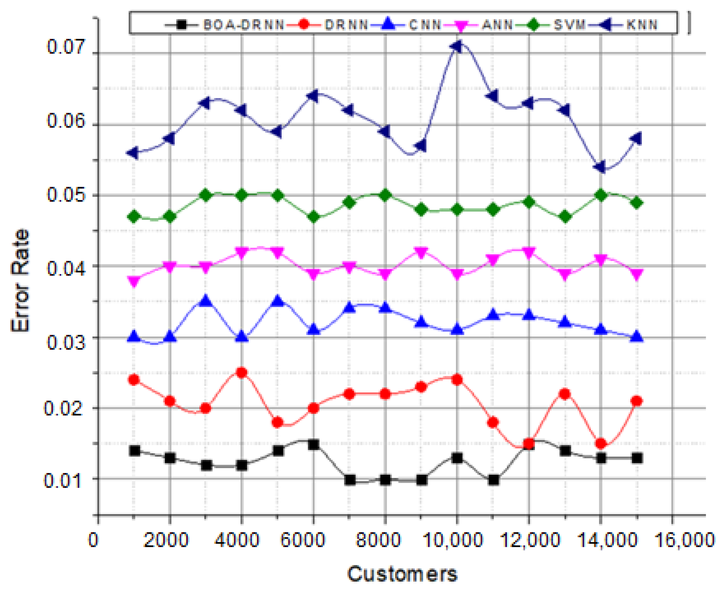
After the clusters were formed, they were processed using the BOA-DRNN. The network predicts customer behaviors according to network learning functions. During this process, the network parameters were updated by applying a BOA. This updating process reduced the maximum error rate classification problem. The continuous network updating process reduces computation complexity and error rates. The prediction system performance was evaluated using different metrics, such as error rate, sensitivity, specificity, F-measure, and accuracy. The acquired results were compared to other single-model-based prediction models, such as KNN, SVM, DNN, and CNN. To ensure optimal validation, four classifiers were implemented. The system used the tuning parameters shown in

Table 2. Tuning Parameters.

Hyper-Parameter	Dataset 1	Dataset 2	Dataset 3
Number of hidden layers	Two	Two	Two
Number of neurons	5	5	5
Training	Gradient decent with momentum
Learning rate	0.0025	0.0020	0.0022
Number of embedding dimensions	300	300	300
Number of nodes in cells	200	200	200
Recurrent dropout keep probability	1.00	0.35	1.00
Batch size	512	256	256
Number of epochs	200	200	200

.

The deviations between the actual and predicted values were computed. A graphical analysis of the error rate is shown in Figure 6. This figure illustrates the error rate values of actual versus predicted customer behavior patterns. Here, the network uses the memory state for every processed input. The network predicts the output in every layer to reduce the number of deviations because it utilizes the network parameters. Furthermore, the network parameters were updated according to butterfly optimization characteristics ${\mathit{b}}_{\mathit{u}}^{\mathit{it}+1}{=\mathit{b}}_{\mathit{u}}^{\mathit{it}}+\left({\mathit{rnd}}^2{\ast \mathit{b}}_{\mathit{v}}^{\mathit{it}}{-\mathit{b}}_{\mathit{w}}^{\mathit{it}}\right){\ast \mathit{fr}}_{\mathit{u}}$ to mitigate the maximum error rate classification problem. Here, the effectiveness of the system was evaluated using different numbers of customers. The minimum error value directly indicated that the introduced system attained high recognition accuracy.

The overall effectiveness of the system results is illustrated in

Table 3. Efficiency Analysis.

Metrics	Dataset 1
	KNN	SVM	DNN	CNN	DRNN	BOA-DRNN
Sensitivity	67.56	72.92	79.35	83.93	93.4	96.87
Specificity	68.36	79.63	77.99	84.24	94.82	97.38
F1-measure	67.46	81.24	79.59	82.34	95.53	98.28
Precision	68.32	81.02	77.34	82.31	94.23	98.12
Accuracy	68.67	83.73	76.23	85.29	93.93	97.51
	Dataset 2
Sensitivity	68.94	73.02	78.35	84.1	93.76	96.98
Specificity	68.92	79.21	78.34	84.134	94.21	97.15
F1-measure	68.34	82.93	79.13	83.54	94.89	97.98
Precision	68.28	81.23	76.28	82.39	95.39	97.23
Accuracy	68.86	83.21	77.34	85.62	94.22	97.33
	Dataset 3
Sensitivity	67.34	74.92	76.38	83.29	92.57	97.34
Specificity	67.92	80.24	79.38	85.244	93.82	97.65
F1-measure	68.84	81.34	80.24	81.46	93.9	98.23
Precision	69.12	83.22	79.28	80.39	93.12	97.2
Accuracy	69.34	82.86	78.35	85.83	94.12	97.98

. From the table, it can clearly be seen that the introduced approach attained the highest accuracy values compared to the other methods, with Dataset 1 at 97.51%, Dataset 2 at 97.3%, and Dataset 3 at 97.9%. The obtained results directly indicate that successfully utilizing the network parameters, objective functions, and optimization techniques improved the efficiency of the overall system.

As expected, deep learning methods recorded higher numbers in all metrics compared to classical machine learning methods such as KNN and SVM. However, SVM achieved better results than DNN, whereas those of KNN were the lowest. The CNN achieved high numbers compared to SVM, KNN, and DNN models in all metrics, whereas KNN showed the lowest performance. The analysis using the BOA-DRNN improved the accuracy over the widely used SVM model by over 13.78% in Dataset 1, 14.12% in Dataset 2, and 15.12% in Dataset 3. SVM is widely used for prediction-related problems because of its usability and the high interpretability of the produced results. This improvement in the predictive performance of the BOA-DRNN can be attributed to its neural network hyper-parameters (weight, number of layers, number of neurons in each layer, batch size, and number of epochs). The tuning of these hyper-parameters has a strong impact on improving the performance.

The multiple network layers of the DRNN improved the process of feature learning [41]. Simple features were learned by the initial layers, whereas the later layers were intended to predict the output according to complex combinations of features. Moreover, the network architecture of the DRNN makes it less exposed to the issue of dimensionality, unlike machine learning techniques [42]. The deep structure of the DRNN enables it to process larger datasets in an efficient manner. The results indicate that, following BOA-DRNN and DRNN, the CNN was able to outperform the others on all explored metrics, with accuracies of 85.29, 85.62, and 85.83 for Datasets 1, 2, and 3, respectively. According to the results, the performance scores of the CNN structure were higher than those of the DNN structure. It is understood that the performances of the two methods are similar in customer behavior prediction problems. Moreover, in such datasets, the number of input features is excessive for a normal DNN structure, which leads to an increase in processing time. In contrast, CNN does not suffer from a large number of features and has a significant advantage because of the feature extraction layer. Therefore, the CNN structure is suitable for problems with large input features, such as customer behavior prediction.

Specificity denotes the portion of negative cases that were classified correctly, while sensitivity denotes the portion of positive cases that were correctly identified. Notably, from Table 3, BOA-DRNN outperformed the other methods in terms of sensitivity and specificity. BOA improved sensitivity by 3.47%, 3.58%, and 4.77% for Datasets 1, 2, and 3, respectively. In addition, using BOA, the specificity increased by 2.56%, 2.94%, and 3.74% for Datasets 1, 2, and 3, respectively. Notably, there was a large increase in both sensitivity and specificity with a minimum 10% difference when comparing BOA-DRNN with the second-best model, CNN. This can be attributed to the fact that RNNs can use their internal memory to process random sequences of inputs.

According to the precision metric, the introduced approach recognizes customer behavior effectively compared to the other metrics. The high precision value indicates that the system clearly exacts output collated with other metrics. The BOA approach increased the precision value by up to 4.128%, 1.92%, and 4.38% for Dataset 1, Dataset 2, and Dataset 3, respectively.

Moreover, unlike deep learning models, SVM and KNN are capable of directly handling categorical variables [15]. Basically, SVM has a smaller number of hyper-parameters compared to neural network models, which makes it easier to tune [14]. Further, the training time for SVM is lowest. Operational efficiency should be considered, as businesses need to predict customers in real time. This is a trade-off between processing efficiency and processing time.

6.3. Hybrid-Model-Based Customer Prediction Models

In this experiment, the proposed approach was compared to other existing hybrid customer prediction models mentioned in the literature, such as PPFCM-ANN [25] and IFNN [24]. The performance metrics used here were mean square error rate (MSE), sensitivity, specificity, F-measure, precision and accuracy.

The effectiveness of the system was evaluated using the three datasets, and the respective results are illustrated in

Table 4. Efficiency Analysis.

Metrics	Dataset 1
	IFNN	PPFCM-ANN	BOA-DRNN
Sensitivity	84.76	93.76	96.87
Specificity	83.92	93.86	97.38
F1-measure	85.24	95.12	98.28
Accuracy	86.34	94.56	97.51
Precision	84.11	93.52	98.12
MSE	0.075	0.0312	0.0124
	Dataset 2
Sensitivity	84.07	93.12	96.98
Specificity	83.17	92.57	97.15
F1-measure	84.41	94.53	97.98
Accuracy	86	94.13	97.33
Precision	83.73	92.88	97.23
MSE	0.079	0.031	0.0112
	Dataset 3
Sensitivity	83.92	90.41	97.34
Specificity	84.26	91.75	97.65
F1-measure	83.89	91.47	98.23
Accuracy	85.23	90	97.98
Precision	84.09	91.24	97.2
MSE	0.098	0.045	0.0103

. For the three datasets, the introduced BOA-DRNN approach attained the maximum prediction accuracy compared to the other methods (Dataset 1: 97.51%, Dataset 2: 97.33, Dataset 3: 97.98%). Followed by PPFCM-ANN, the BOA-DRNN raised the accuracy with 2.95, 3.2, and 7.98 for Dataset 1, Dataset 2, and Dataset 3, respectively. The difference increased gradually along with dataset size, which makes our hybrid model preferable for larger datasets. Specificity denotes the portion of negative cases that were classified correctly while sensitivity denotes the portion of positive cases that were correctly identified. Notably, BOA-DRNN outperforms the other methods in terms of sensitivity and specificity. According to sensitivity, our model achieved the following results: Dataset 1: 96.87, Dataset 2: 96.98, and Dataset 3:97.34. In specificity, BOA-DRNN achieved the following results: Dataset 1: 97.38, Dataset 2: 97.15, and Dataset 3: 97.65. Furthermore, the maximum precision was achieved by BOA-DRNN followed by PPFCM-ANN with differences of 4.6, 4.35, and 5.96 for Dataset 1, Dataset 2 and Dataset 3, respectively. Clearly, IFNN was the lowest performance compared to the other two hybrid models. The MSE numbers were low for all the examined hybrid models. There were only slight differences between them, with BOA-DRNN being the lowest.

The BOA-DRNN network uses the clusters formed by a DBN with HFC as the input to identify customer behavior. Here, the belief network had a set of layers that processed the network according to the learning function. The optimization algorithm was then applied to reduce the deviation between the actual and predicted values. In addition, the optimization algorithm updated the network parameters to regularize network performance effectively.

7. Conclusions

Customer behavior prediction is vital to the improvement of companies’ service quality and growth. Gathered customer data need to be processed by applying different machine learning techniques to predict behavior patterns. This study analyzed customer data by using a novel hybrid model of DBN-HBL clustering with an optimized deep neural network approach. The network used visible–hidden layer pair information, and the respective probability values were computed. According to the probability value, clusters were formed. The clusters were then transmitted to the optimized DRNN to determine customer purchasing behaviors. All the experiments were based on three benchmark datasets. Here, the maximum error rate classification problem and overfitting were resolved by updating the network parameters using the BOA. The system was compared to single-model-based approaches such as KNN, SVM, DNN, and CNN. In addition, a comparison with other hybrid-based models was conducted. The system ensured high accuracy and outperformed them according to respected evaluation metrics. Even though the proposed models attained high performance, they do not consider customer feature importance or how these features affect prediction output. Future works can investigate the impact of such features on machine learning models to help businesses increase their success. In the future, more advanced optimization mechanisms for feature selection and deep neural network optimization will be recommended to examine their adaptability in predicting customer behavior. Moreover, advanced hybrid models should be considered to achieve higher prediction performance for customer behavior. A variety of datasets should be examined within an experiment due to the nature of data affecting the training and performance of machine learning models. Other mechanisms to reduce bias can also be investigated to decrease processing time.