1. Introduction
Wireless sensor networks (WSNs) provide us with a cost-effective way to remotely monitor a large number of objects, locations, and environmental parameters [
1,
2,
3,
4,
5]. New technologies and applications for WSNs have been continually proposed, since monitoring capability is becoming more important than ever. For example, pervasive games [
6] and sport training [
7] are recent examples of applying WSN technologies to provide new services in our daily life. Surely, further taking advantage of WSNs for applications can add new capabilities to existing products and bring out new services. The challenge is to have sufficiently low setup, operation, and maintenance costs.
In WSN applications, especially in outdoor environments, how the wireless sensor node determines its location is an important issue. It will be meaningless if the measurement data do not include the node’s location information. For cost-effective consideration, it is likely that not all wireless sensor nodes have the capability to determine their locations only by themselves. In the early days, only a small number of wireless sensor nodes could specifically have the complete capability to determine their locations, i.e., they were anchor nodes with GPS receivers. Other wireless sensor nodes then computed their estimated locations with the assistance of signals/beacon messages broadcasted from anchor nodes. Depending on the balance among cost, precision, and complexity, different kinds of localization schemes have been proposed [
8,
9,
10,
11,
12,
13,
14,
15,
16,
17,
18,
19,
20]. As hardware cost is rapidly falling, it is expected that a larger ratio of wireless sensor nodes can have complete localization capacity. Nevertheless, the localization problem for common wireless sensor nodes is still important. However, the approaches to solving this problem may be more direct and simpler.
Localization schemes can be categorized as range-based and range-free schemes. In range-based schemes, the computation of a node’s location largely relies on the measured distances to anchor nodes. Common distance measurement methods include time of arrival (TOA), time difference of arrival (TDOA), angle of arrival (AOA), and receiver signal strength index (RSSI) [
8]. Range-based schemes are not frequently employed due to the equipment cost and sensitivity to environmental factors. In range-free schemes, a wireless sensor node is not required to measure the distances between it and anchor nodes. Instead, indirect methods are used for estimating the node’s location. Intuitive methods include using the centroid of all locations of direct detected anchor nodes as the estimated location [
9]. As performance fluctuates easily with many factors such as anchor node distribution, different kinds of approaches are proposed. For example, one may have the estimated distances to anchor nodes if the information of average hop number to anchor nodes is available [
10,
11]. This increases the communication overhead and narrows the choice of routing schemes for WSNs, but a smaller number of anchor nodes is generally required. Another shortcoming of such approaches is that the distribution of all wireless sensor nodes, not only anchor nodes, will interfere with the accuracy of location estimation. Surely if extra communications between common wireless sensor nodes and anchor nodes are feasible, the performance of location estimation can be largely improved [
12]. Without the assumption of extra communications, there are approaches that use areas of shapes computed from locations of anchor nodes and strengths of received signals to estimate locations [
13,
14,
15]. Such approaches require rather primitive information from anchor nodes, but a large number of anchor nodes is commonly assumed. From this aspect, they are likely more appropriate for coming WSN scenarios, with large ratios of anchor nodes being available. To have better localization accuracy, however, some of them often need to generate large numbers of areas and others assume good capability of signal receiving. This may limit the practical applications of such approaches in another aspect. In this paper, we therefore propose a Voronoi diagram-based grouping test location (VTL) scheme to simplify the implementation and also improve the performance of location estimation.
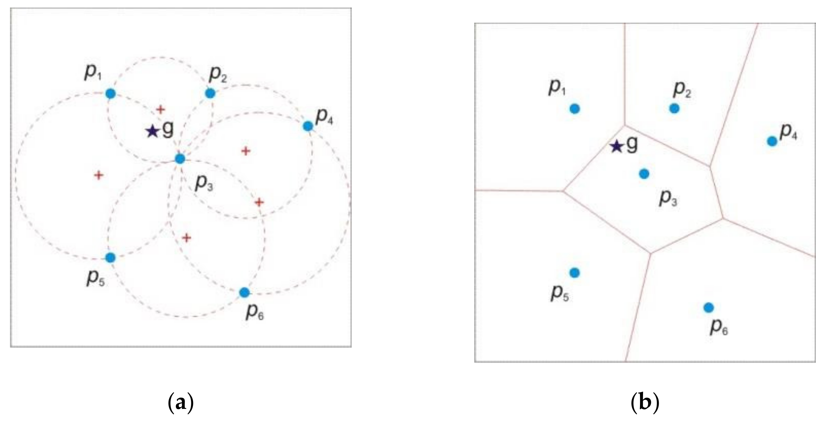
A Voronoi diagram provides us with a handy way to partition a plane. It has been widely applied in site selection, formation control, planning, face recognition, and network optimization [
21,
22]. Efficient algorithms are freely available for generating Voronoi diagrams. This largely simplifies the use of Voronoi diagrams in different algorithms. Furthermore, Voronoi diagrams have also been used in other localization schemes to improve the schemes’ performances [
16,
17,
18,
19,
20]. In [
16], Voronoi diagrams were used to limit the flooding messages required for the DV localization schemes. In [
17], a half symmetric lens-based localization algorithm (HSL) was proposed using a Voronoi diagram to further refine the results. In [
18], the indoor localization problem was solved with the radio map (fingerprinting) approach, and Voronoi-based interpolation improved the localization performance. In [
19], the indoor locations of robots were estimated by matching the local laser scan-generated Voronoi diagram (LVD) with the global Voronoi diagram. In [
20], the authors proposed a fingerprinting-based localization approach in conjunction with a Voronoi diagram to estimate the location in indoor parking lots. From the above review, one can observe that the Voronoi diagram is not the core technique for location estimation. In this paper, however, we only use the basic Voronoi cell feature and minimal radio signal detection for a VTL localization scheme. In
Section 2, some foundations of VTL are briefly discussed, including the Voronoi diagram, the logarithmic attenuation model for radio signals, and the basic idea of VTL.
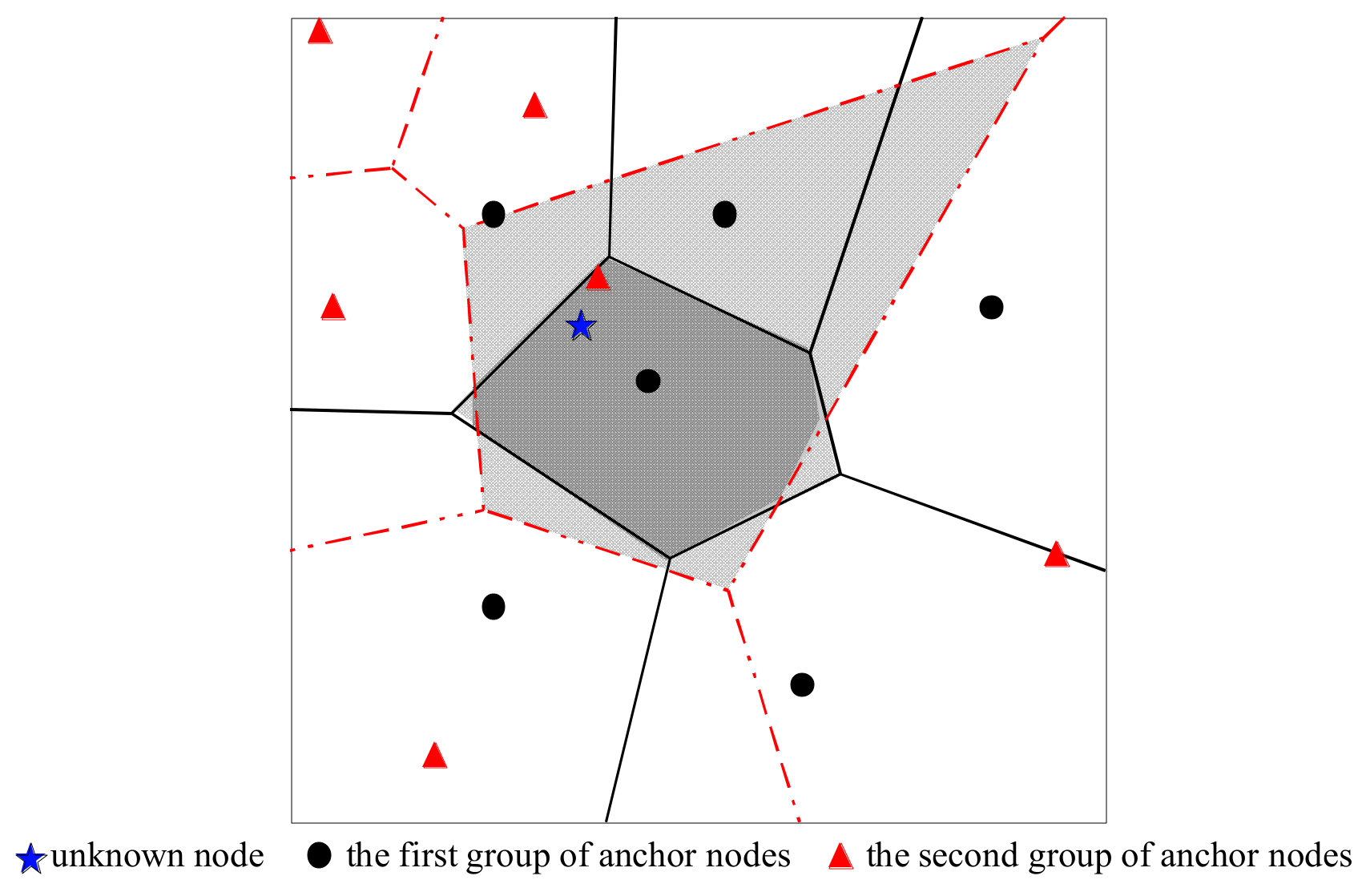
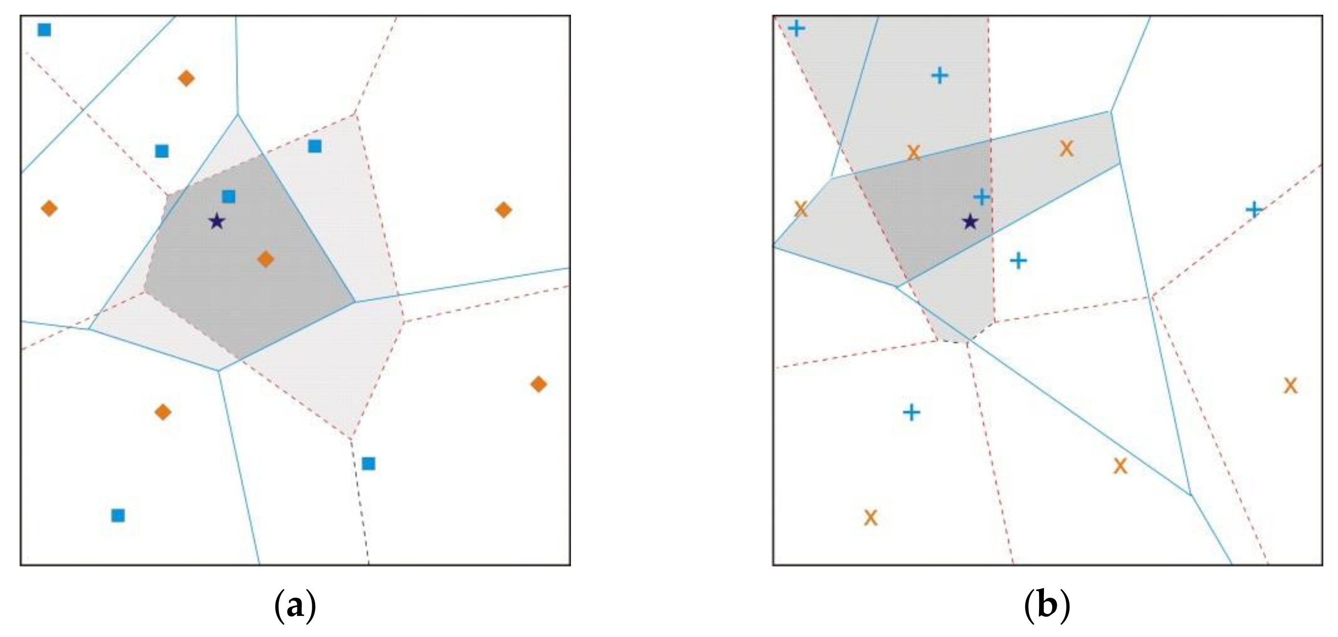
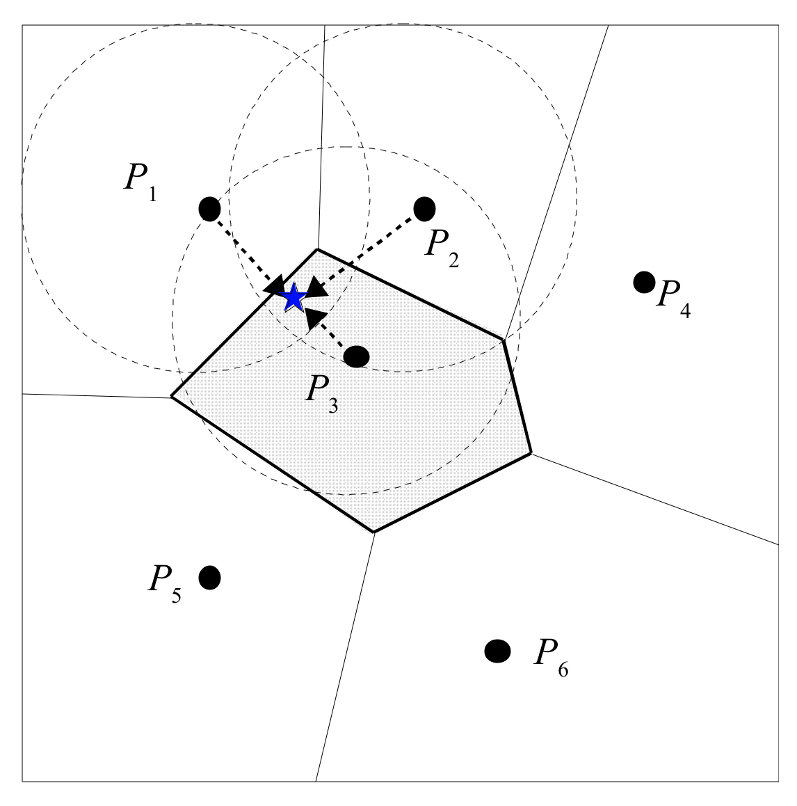
Section 3 then goes through the VTL scheme in detail. The novelty of VTL is the proposed approach of generating multiple Voronoi diagrams with the same set of anchor nodes. Overlapping the closest Voronoi cells from the multiple Voronoi diagram provides us with more accurate location estimation.
Section 4 presents simulation experiments and analysis. In
Section 5, the possible application scenarios for VTL and implementation issues are discussed.
4. Simulations and Analysis
We conducted extensive virtual experiments using MATLAB as the simulation platform to test the performance of the VTL scheme. Performance evaluations at different sensor deployments were discussed. Two localization schemes, Centroid localization [
8] and APIT [
12], were used for comparison. The APIT scheme uses a randomly composed triangle of anchor nodes communicating with unknown nodes, and Centroid localization is a typical indirect estimation (range-free) localization scheme. The performance of the three localization schemes was visualized through average estimation error (
Ea) and estimation percentage (
Pe), given in (8) and (9).
where
and
represent the number of total unknown nodes and localizable unknown nodes, respectively.
denotes the actual coordinates of node
.
denotes the ratio of the average positioning error of nodes to the communication radius
R, which indicates the positioning accuracy of the algorithm.
demonstrates the percentage of localizable nodes.
4.1. Settings of Simulation Parameters
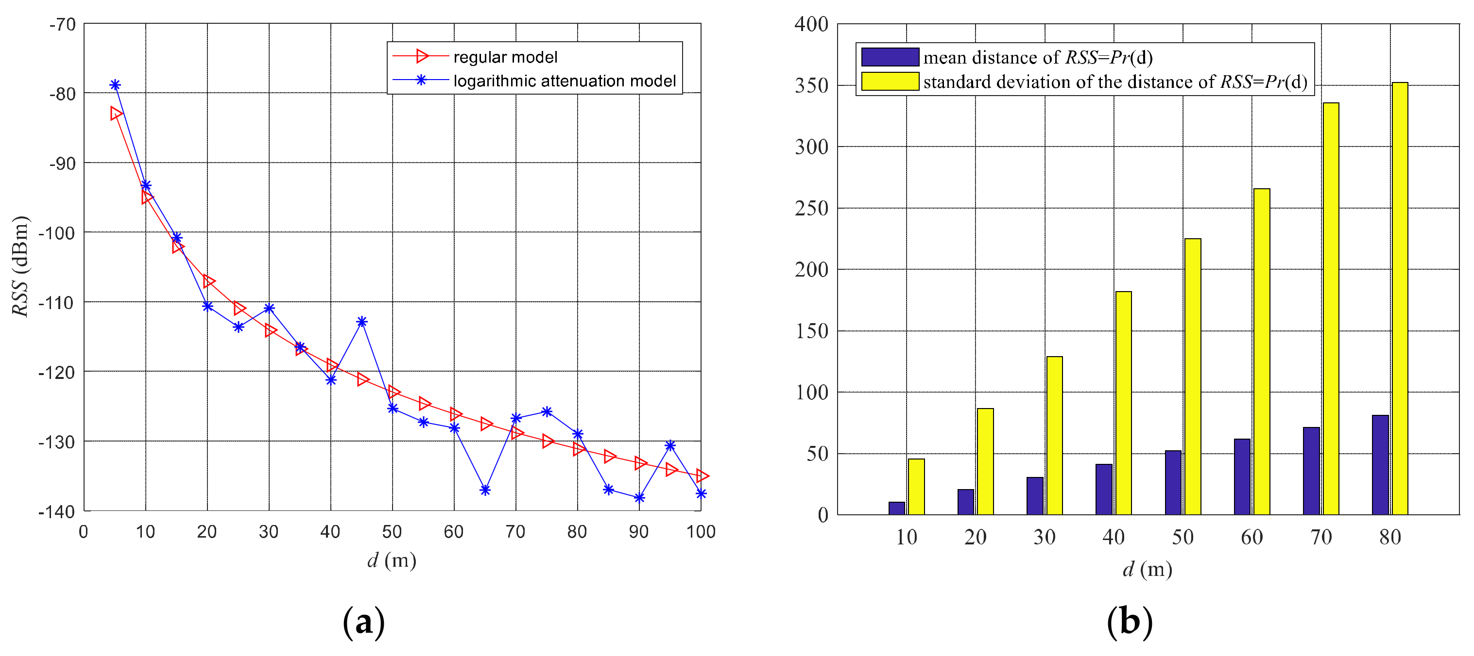
Assuming that the virtual experimental environment is in an open outdoor area, the performance of the VTL scheme was evaluated with a square topology in which wireless sensor nodes were randomly distributed with uniform probability distribution. We used the radio signal model (i.e., (3)), as discussed in
Section 2.2, and
Table 1 lists the parameters that are commonly used for WSN simulations. We studied several parameters that may directly affect the performance of range-free schemes, as shown in
Table 2.
Let
Nt =
Na +
Nu be the number of total nodes. The ratio of anchor nodes
is the proportion of anchor nodes to the total number of nodes, as written in (10).
The GPS error () refers to the maximum error introduced by GPS equipment when acquiring positions of anchor nodes. In this paper, we assumed that GPS errors are isotropic.
4.2. Number of Groups
In
Figure 8, the effect of the number of groups (
) changing from 2 to 10 on
and
is illustrated. Though we did not plot the case of
K = 1 in the figure, we observed that dividing the anchor nodes into multiple groups can improve the accuracy of location estimation. It can be seen that the change in
was rather minor when
was varied. However, the value of
kept decreasing as
was increased. When
= 6, the decreases in
became negligible. Therefore, in the following experiments, we chose
.
4.3. Density of Nodes
In this section, we explored the effect of density of nodes on the VTL scheme at four different setups, as shown in
Table 3.
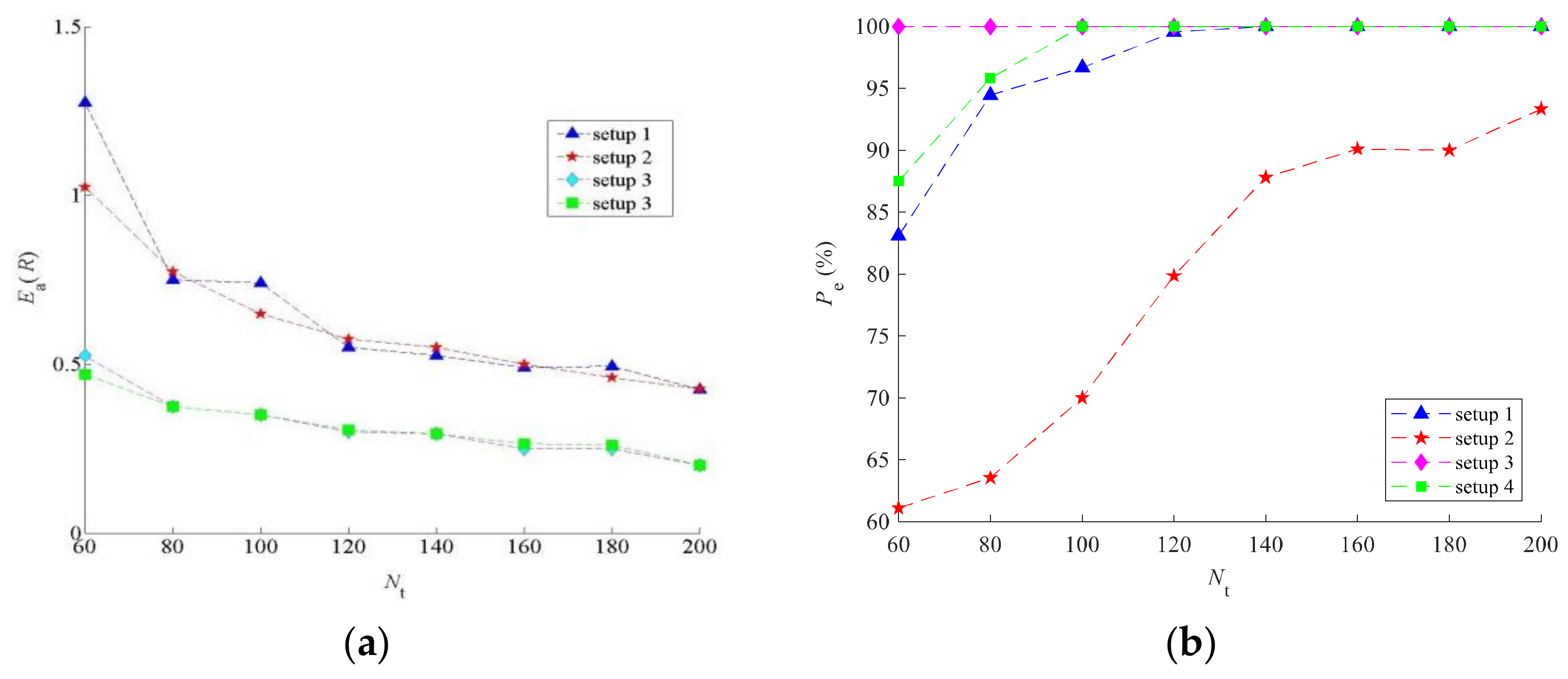
As shown in
Figure 9a,b,
Ea decreased but
increased when
varied from 60 to 200 in all four situations. We had the worst
Ea and
Pe with setup 2. With the increases of density of nodes, unknown nodes could receive more beacon messages from anchor nodes, which therefore improved the location accuracy effectively. Note that the effect of node density on the VTL scheme was mainly due to the increase of anchor node density. VTL does not rely on the communications between unknown nodes, i.e., it is insensitive to unknown node density.
4.4. Performance Comparisons with Square Topology
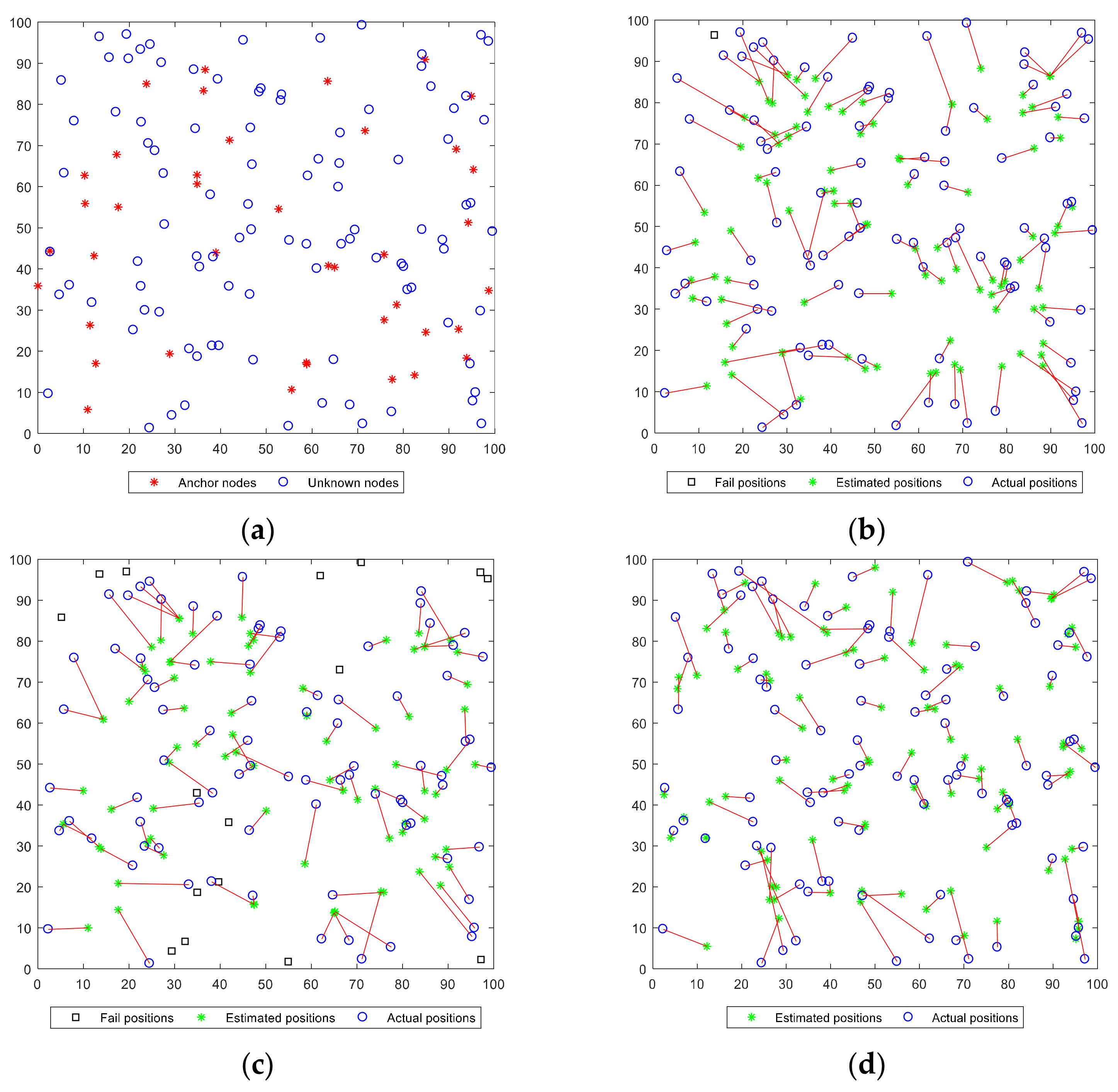
A comparison of simulation outcomes of three range-free schemes (VTL, APIT, and Centroid) is shown in
Figure 10. As it may not be easy to compare the performance of different schemes from
Figure 10, we list the statistical data in
Table 4. We observed that the VTL algorithm proposed in this paper outperformed both in localization accuracy and percentage of localizable unknown nodes. Apart from
Figure 10, we compared the performance of the three schemes by varying other parameters such as anchor node ratio, communication radius, and GPS error rate in the following sections.
4.4.1. Anchor Node Ratio
The parameters set for the simulation environment were an area of 100 × 100 (
),
EGPS of 0.1 m,
R of 20 m, and
of 100. In this section, anchor nodes were randomly arranged in a uniform probability distribution. The randomness was reflected by the one-to-one correspondence between the position coordinates of anchor nodes and two-dimensional random numbers. As shown in
Figure 11, the effect of the ratio of anchor nodes on the three schemes with respect to
and
is illustrated. As can be seen in
Figure 11a,
of three algorithms kept increasing. We observed that
of the VTL algorithm was always the highest. As can be seen in
Figure 11b, when
was less than 30%, the error of VTL was larger because most the unknown nodes in the VTL scheme could complete the estimation with only one beacon message, but
was larger in this case, while more beacon messages needed to be obtained in the Centroid and APIT schemes. When
varied from 10% to 70%,
of the VTL scheme fell the most. As a result, VTL improved the level of location accuracy while maintaining a high positioning coverage rate.
4.4.2. Communication Radius of Anchor Nodes
The larger the communication radius
Ra of the anchor node, the more unknown nodes can be covered by beacon messages, which is equivalent to increasing the density of anchor nodes and is conducive to reducing costs. In this part, we studied the influence of the anchor node radius
Ra on localization accuracy, as shown in
Figure 12. We observed that the estimation errors of Centroid and APIT increased greatly, while VTL barely increased when
Ra became larger. The reason why the
of Centroid and APIT increased when varying
is that larger beacon propagation distances result in a larger accumulated error (see the discussion with
Figure 2). In these two schemes, each beacon message was equal in estimating the location of unknown nodes. On the contrary, in VTL, only the closest anchor node was needed to find a “positive region” in each group of anchor nodes. Beacons from farther anchors will have no influence on VTL unless the error in
Rss is sufficiently large to cause the wrong closest anchor nodes to be chosen. As all radio signal strengths increase simultaneously, an unknown node’s choice of its closest anchor node will not change. Therefore, the VTL scheme is insensitive to the increase of
.
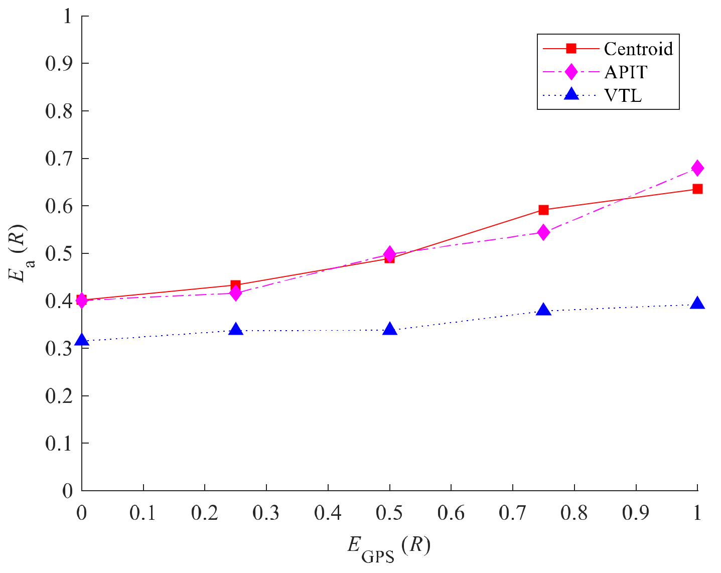
4.4.3. GPS Error
In reality, randomly distributed anchor nodes use GPS circuits to obtain their own position. In order to make the simulation experiment more comprehensive, we explored the effect of
EGPS in this section with
equal to 20 m. The simulation result is shown in
Figure 13.
As the EGPS varied from 0 to 20 m, the errors of all schemes increased. This is because the location of the anchor node was used as a reference for estimating the location of an unknown node, which affected the location accuracy directly. Nevertheless, the growth rate of Ea was lower than that of EGPS, and that of the VTL scheme was the lowest. In general, Ea was rather insensitive to GPS errors.
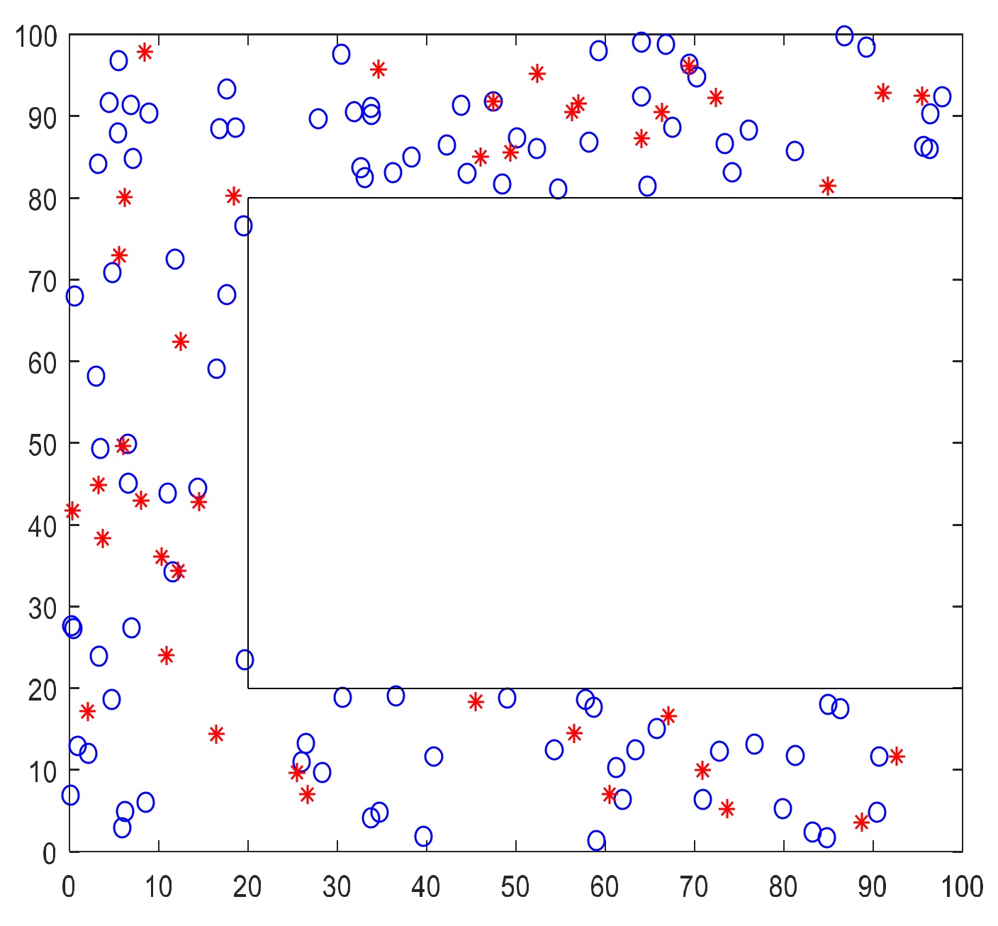
4.5. Performance Comparisons with C-Shaped Topology
To further investigate the features of the VTL scheme, simulations were arranged with the C-shaped topology, as seen in
Figure 14. The C-shaped topology was generated by removing a small rectangle (80 × 60 m
2) from a large square (100 × 100 m
2). Its total area was only 52% of the square topology in
Figure 10. In
Figure 14, there are in total 140 nodes (100 unknown nodes (circles) and 40 anchor nodes (asterisks)). Its node density is approximately double that of the square area in
Figure 10. One should also be aware that the radio signals sent from the anchor nodes are not bounded by the boundary of the area, no matter the square topology in
Figure 10 or the C-shaped topology in
Figure 14. This point has no significant effect on the simulation results of
Figure 10 but has impacts on the C-shaped topology in
Figure 14. Moreover, we assumed that the Voronoi diagrams can only be drawn inside the area of C-shaped topology.
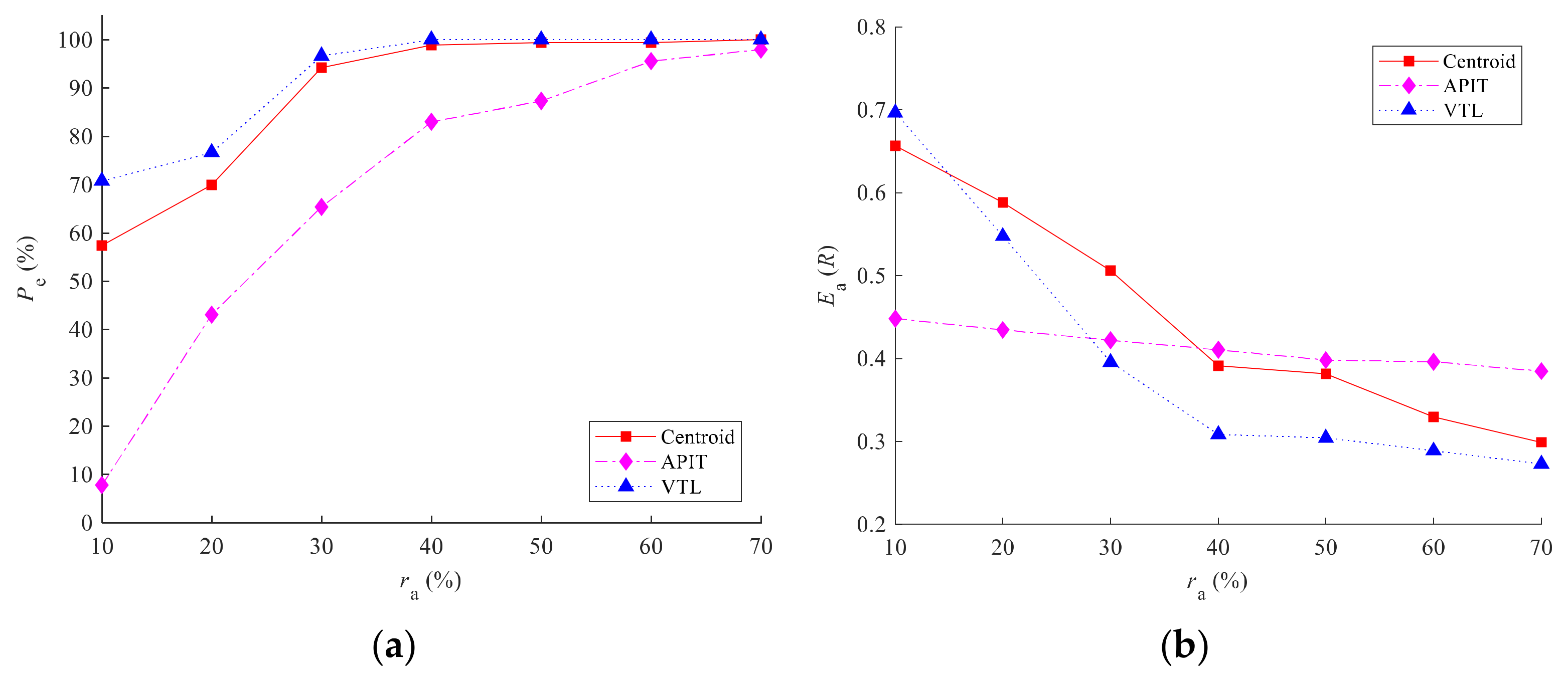
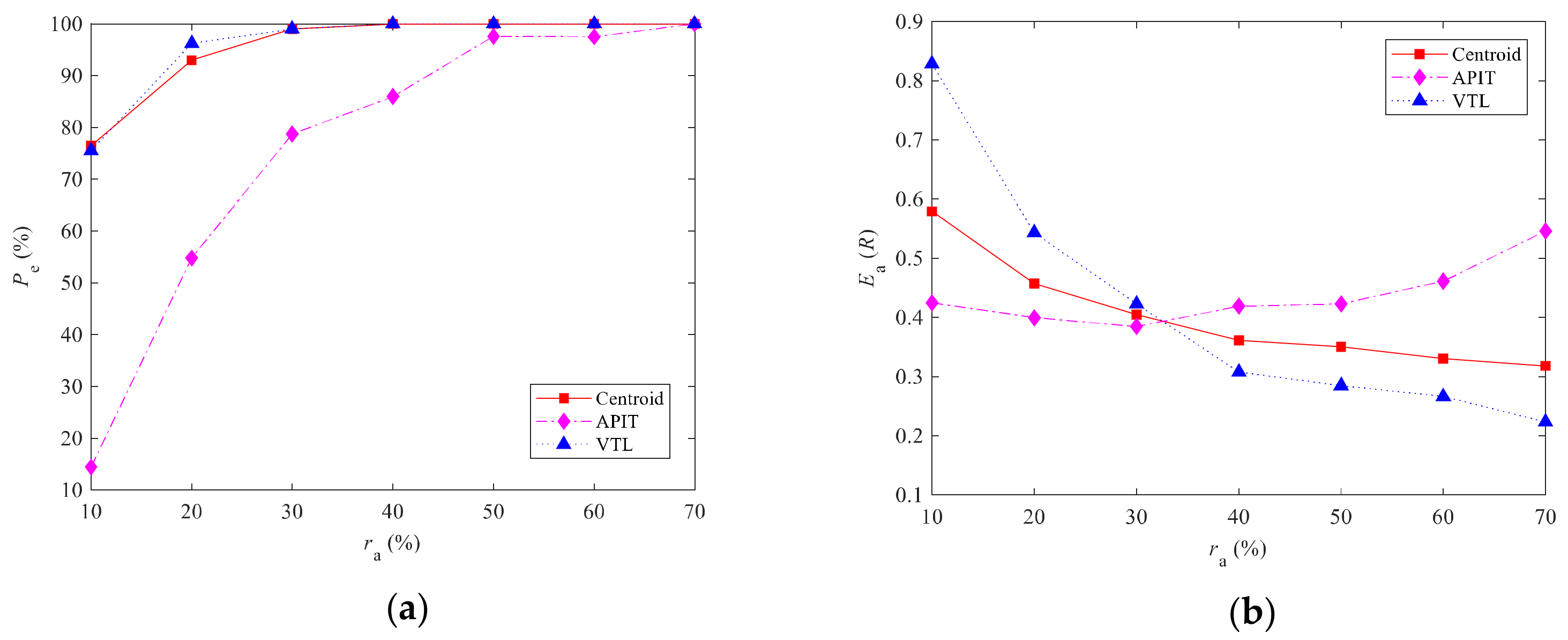
Figure 15 shows the effect of the ratio of anchor nodes
ra on three schemes (VTL, APIT, and Centroid). We increased
ra from 10% to 70% and plotted the estimation percentage (
Pe) and estimation error (
Ea). Comparing
Figure 15 with that of
Figure 11, one can observe that
Pe of all schemes in the C-shaped topology was higher. Moreover, the
Pe of Centroid was closed to that of VTL. This was due to the smaller effective area and higher node density. For
Ea performance, those of APIT first slightly decreased but increased again after
ra exceeding 30%, which is because APIT used the overlapping area of triangles formed by detectable anchor nodes to estimate locations. The number of triangles increases with
ra, but some of them may have had areas outside the boundary of the C-shaped topology. Hence, increasing
ra can improve
Pe of APIT but may degrade its
Ea performance. Both Centroid and VTL had their
Ea decreasing with
ra. From the range 10% to 35% of
ra, however, the performance of Centroid was better than VTL, which is because Centroid used the centroid of all detectable anchor nodes to estimate an unknown node’s location. Since Voronoi diagrams must be drawn within the boundary but the boundary does not block radio signals, Centroid may have an advantage unless the density of Voronoi cells is sufficiently high for VTL. Evidently, the performance improvement of VTL is faster than Centroid with increases of
ra even though it is an irregular topology network, e.g., the C-shaped topology. Moreover, one can make the same observation from
Figure 11, i.e., VTL has better
Ea performance than Centroid when
ra exceeds 15%.
5. Conclusions and Discussion
In this paper, we proposed a novel range-free localization scheme, the Voronoi diagram-based grouping test localization (VTL) scheme, to estimate the location efficiently for wireless sensor networks (WSNs). Unlike many other schemes, VTL only relies on the information broadcasted from static anchor nodes. No communication between nodes is required. The number of locatable unknown nodes can therefore be greatly increased. VTL divides the anchor nodes into multiple groups and uses the corresponding Voronoi cells to compute the estimated location. Apart from improving the accuracy of location estimation, it also largely simplifies the implementation because efficient algorithms are freely available.
From simulation results on regular and irregular network topologies (i.e., square and C-shaped topologies), it shows that VTL will have better performance compared with other range-free localization schemes when it reaches a certain anchor node density, e.g., 30% in the simulations. Hence, a possible application scenario of VTL will be for the extension of an existing WSN with most of the nodes having localization capacity. With VTL, the added sensor nodes do not need sophisticated hardware for communications and localization. Instead, a minimal computational capability is still required for solving the Voronoi diagrams, which grows with O(NalogNa), where Na is the number of original nodes being used as anchors. As computational hardware is continuously improving and the cost is rapidly falling, it should not be an issue for VTL in the coming future. One advantage of VTL is that its location estimation accuracy always grows with the number of anchor nodes. Other range-free localization schemes may not have such features.


 ,
, 


