Learning Balance Feature for Object Detection

Abstract

In the field of studying scale variation, the Feature Pyramid Network (FPN) replaces the image pyramid and has become one of the most popular object detection methods for detecting multi-scale objects. State-of-the-art methods have FPN inserted into a pipeline between the backbone and the detection head to enable shallow features with more semantic information. However, FPN is insufficient for object detection on various scales, especially for small-scale object detection. One of the reasons is that the features are extracted at different network depths, which introduces gaps between features. That is, as the network becomes deeper and deeper, the high-level features have more semantics but less content description. This paper proposes a new method that includes a multi-scale receptive fields extraction module, a feature constructor module, and an attention module to improve the detection efficiency of FPN for objects of various scales and to bridge the gap in content description and semantics between different layers. Together, these three modules make the detector capable of selecting the most suitable feature for objects. Especially for the attention module, this paper chooses to use a parallel structure to simultaneously extract channel and spatial attention from the same features. When we use Adopting Adaptive Training Sample Selection (ATSS) and FreeAnchor as the baseline and ResNet50 as the backbone, the experimental results on the MS COCO dataset show that our algorithm can enhance the mean average precision (mAP) by 3.7% and 2.4% compared to FPN, respectively.

1. Introduction

In the field of computer vision, detecting instances of various scales is a challenging task. Image pyramids are proposed to detect various scale objects by feeding the same images with different resolutions into the network, such as SNIP [1,2,3]. However, the training and inference of image pyramids also incur high computational costs. Compared with the image pyramids, the Feature Pyramid Network (FPN) [4] takes a single scale image as input and extracts features of different resolutions from different network depths. Each resolution feature can be used to detect objects of a certain scale. However, since most backbone networks for object detection are designed for classification tasks, such as ResNet [5], ResNeXt [6], etc., features at different network depths have different semantic representation capabilities. This is the semantic gap between high-level and low-level features [3,7,8]. On the other hand, as the network becomes deeper and deeper, the resolution of the features becomes smaller and smaller, and the location information of objects is gradually lost [9]. As a result, the deep high-level and shallow low-level features of FPN have an imbalance of semantic and location information, making it difficult for the detector to enhance performance.

By observation, high-level features with low resolution have fewer location details but more semantic information. Conversely, low-level features with high resolution have fewer semantics and more location information. Intuitively, the most straightforward way is to fuse high-level and low-level features to generate balanced features.

The first method is to extract features from deeper and wider backbones, such as ResNeXt [6], or task-specific backbones, such as HourglassNet [10] for semantic segmentation and HRNet [11] for object detection. A deeper and wider backbone network always leads to higher computing costs. The FLOP of HRNet is 32.9 G, while that of ResNet50 is 3.8 G.

The second way is to sequentially fuse the features extracted from the backbone through a specific path, such as FPN with a top–down path and Path Aggregation Network (PANet) [12] with a bottom–up path. Due to the sequential way, the information is gradually attenuated during the fusion, so the features of the bottom layer or the top layer cannot receive enough information from the top layer or the bottom layer.

The third way is to resize the features of different resolutions to a specific scale by up-sampling or down-sampling, and then fuse all the features into one. For example, the Balance Feature Pyramids (BFP) of Libra RCNN [13] combine all the features from different layers into one. The PConv of Scale-Equalizing Pyramid Convolution (SEPC) [14] only fuses adjacent feature layers. When fusing features in BFP or PConv, they are given the same weight regardless of whether they are derived from separate layers with distinct semantics and content descriptions.

Inspired by the fact that the same object is most likely to be detected in adjacent feature layers, this paper exploits the correlation between adjacent feature layers and proposes a new algorithm to generate balanced features. The new algorithm is named Balance Feature Transformer (BFT). After integrating BFT into ATSS and FreeAnchor, their detection performance is significantly improved.

The main contributions of this paper are summarized as follows:

1.

This paper proposes a new feature fusion method called the Balanced Feature Transformer (BFT), which is based on the correlation between adjacent features of the pyramid. The features output by our method have a better balance in terms of semantic discriminative ability of features and object localization, and at the same time, they have a low computational cost.

2.

To take full advantage of the semantic and location information of different features, this paper also proposes a multi-layer feature attention algorithm that learns different types of attention from the same feature through two parallel branches, thereby enhancing the ability of the detector to detect objects.

3.

Our method has low computational cost and can be easily embedded into existing algorithms. This paper achieves a 3.7 AP improvement on the SOTA algorithm ATSS.

2. Related Work

2.1. Deep Object Detector

Convolutional neural networks (CNN) have achieved great success in object detection. CNN-based object detection is a very important topic in computer vision: for example, multi-object tracking [15], autonomous driving [16], robotics [17], medical image analysis [18], etc. Many edge devices are limited in the computing power, and the deployed models models need to be lightweight.

All the CNN-based detectors can be roughly divided into two categories, i.e., two-stage detectors and one-stage detectors. Two-stage detectors, such as Faster R-CNN [19] and its improvements, divide the whole detection process into two stages. In the first stage, proposals are generated, and then, the second stage determines the accurate object regions and the corresponding class labels according to the proposals. One-stage detectors, e.g., YOLO [20], follow an end-to-end manner to classify and locate objects on features without the region proposal step. Compared with the two-stage detector, the one-stage detector has a faster detection speed but lower accuracy. For the two-stage detector, the scale variance problem is alleviated, since the ROI is resized to a fixed size before performing detection.

Detectors can also be divided into anchor-free and anchor-based algorithms according to whether anchor boxes are used. The anchor-based algorithm is used to lay out anchor boxes on the features. However, the anchor box parameters, such as height and width, need to be manually designed for new scenarios with different object sizes or aspect ratios. Anchor-free detectors learn to recognize keypoints of instances, such as center points or corner points, rather than using anchor boxes to detect instances. Typical anchor-based algorithms include YOLO [19,21], SSD [20] and so on. FoveaBox [22] and CornerNet [23] detector are two typical anchor-free algorithms.

How to select positive and negative samples greatly affects the performance of the detector. The SOTA detectors, ATSS and FreeAnchor, use two different strategies for selecting positive samples and negative samples. This article chooses the one-stage, anchor-based detector ATSS as the first baseline. ATSS computes the mean and deviation of the IOU between all predicted boxes and ground truth boxes, thereby adaptively calculating the thresholds for positive samples. A second baseline detector is FreeAnchor, which uses maximum likelihood estimation (MLE) as a way to learn how to identify positive and negative samples. Both algorithms are one-stage, anchor-based detectors that lay out anchor boxes identically but differ in how they determine if the sample is positive or negative. Most of the experiments are performed on both methods to verify how well the detectors perform after integrating our BFT method.

2.2. Feature Receptive Field

To detect objects of various scales, extracting features from images with different receptive fields is a very intuitive method. However, the effective receptive field [24] is proportional to the network depth and the size of the convolution kernel. ASPP [25] employs different-sized convolution kernels to extract features with various receptive fields. RepVGG [26] uses large convolution kernels to extract features and obtain large receptive field. In this paper, we hope that the features have different receptive fields, and there can be some cooperation between the features to jointly detect objects of different scales. So, we propose the multiple receptive fields feature extractor (MRFE) module to fuse features with different receptive fields together.

MobileNet [27] uses depthwise separable convolution and pointwise convolution to extract features. We consider using a simple network structure to achieve low computational cost and multi-receptive field features. Therefore, we choose dilated convolution as the basic module to construct MRFE. Dilated convolution can use fewer parameters and extract larger feature receptive fields.

2.3. Multi-Level Feature Fusion

The input of FPN is a multi-scale feature set with which each feature has different channel numbers, and the output is also a multi-scale feature set, but every feature’s channel number is the same. The FPN has the following defects [28,29]. On the one hand, high-level features suffer from information loss due to feature channel reduction. On the other hand, deep high-level features in backbones have more semantic meanings, while the shallow low-level features are more content descriptive [28]. FPN transfers the high-level features to the low-level features through a top–down path. The semantics gradually decay during this process; thus, the low-level characteristics do not obtain appropriate semantic information. In other words, FPN does not fully exploit the complementarity of the deep and shallow layers to improve the semantics of low-level features.

For FPN or PANet, the main purpose is to balance the semantics and localization information between high-level and low-level features. The information is gradually attenuated due to the downward or upward transmission in a layer-by-layer manner. In order to solve the above problem, Libra R-CNN [13] proposed Balanced Feature Pyramids (BFP), which fuses all output features of FPN together to form a median scale feature and then generates features of the desired scales by resizing. The BFP has to use a non-local [30] attention module to refine the median scale feature. This makes the network difficult to train and has a high computation cost. AugFPN [28] introduced Residual Feature Augmentation (RFA) and Adaptive Spatial Fusion (ASF) modules to improve network performance and alleviate the effects of FPN defects. Meanwhile, RFA and ASF are too complicated, make the network heave and slow down the inference speed. SEPC [14] applied the correlation between the feature levels and proposed to use cross-layer convolution to improve the detection performance on multi-scale features. However, the PConv method treats all features equally and ignores the differences between features during fusion. NasFPN [31] uses Neural Architecture Search (NAS) to search for a better network structure, which greatly improves the detection results, but it is tricky to explain and has a high computational cost. Adaptively spatial feature fusion (ASFF) [32] generates weight for features and adopts an adaptive strategy for feature fusion. However, in this way, there is a significant slowdown on GPU hardware [7], resulting in a significant amount of time to train the network.

The Feature Pyramid Network (FPN) detects objects of various scales through features of different resolutions. However, actually, objects of a certain scale are difficult to detect on some feature layers due to the different receptive fields [33]. For example, it is difficult for small objects to be detected at low-resolution features with large receptive fields. Most of the existing methods achieve feature balance by fusing features from different layers, which ignore feature layer and object scale matching, resulting in inefficient computation. Therefore, we believe that the size of the object should also be considered when alleviating feature imbalance. In order to detect as many objects as possible on one feature layer, we consider using multiple convolution kernels with various kernel sizes to extract features with different receptive fields. Features can adaptively match objects of various scales.

2.4. Task-Awareness Attention

Naturally, since objects of vastly different scales often co-exist in images, how to detect them all is a challenging task in object detection. Traditionally, image pyramids with multi-scale training [1,2,34] are used to detect various scales of objects. Unlike image pyramids, feature pyramids [4] generate a set of features with different resolutions in which objects of various scales are detected. The problem of how to guide the network to extract features that match the object scale becomes important.

Libra R-CNN [13] proposes to insert a non-local module right after the BFP to make the balanced semantic features more discriminative. SEPC [14] introduces a modified 3D convolution PConv to extract scale and spatial features simultaneously. ASFF [32] introduces learnable parameters to conduct feature fusion. ASFF only learns three scalar weights, which is insufficient for the fusion of multi-feature layers. Attentional Feature Fusion (AFF) [35] introduces a new attention module, MS-CAM, to enhance the feature ability of features to detect objects of various scales. MS-CAM uses the self-attention method, which makes it heave. Non-Local is a self-attention module that pays more attention to regions of interest, but the computational cost is high. ASFF learns to choose appropriate features but ignores regions where the instances may be located. The MS-CAM module, with a structure similar to self-attention, extracts channel information through global average pooling and strengthens feature category information, but it pays less attention to object location information.

The object detection task is to tell what an instance is and where it is. Therefore, the network should strive to find the most suitable features for the location and category of objects. We present a task-aware attention method in this paper to help the detector figure out which features are optimal for the input and where the objects are most likely to be found.

3. Method

Figure 1 shows the whole pipeline of Balance Feature Transformer (BFT). The multiple receptive fields feature extractor (MRFE), the feature constructor module, and the multi-layer channel and spatial attention (MLCS) module make up the overall framework. The MRFE module configures convolutions with different kernel sizes and then concatenates them along the channel dimension to form features with different receptive fields. The feature constructor module extracts multiple scale features from each feature layer and combines the same scale features into a new feature layer. The MLCS module extracts the channel and spatial attention from the same features, allowing the detector to pick the appropriate feature layer based on the input image. In the following sections, we will describe all components in detail.

Compared with the Feature Pyramid Network (FPN) and Balance Feature Pyramid (BFP), our method exploits the correlation of adjacent features so that the output features have more discrimination. In the pipeline, we integrate MRFE so that the features have different receptive fields (RF) and make the RF quite different. With the help of MLCS, the features are more balanced. All of these make our method more robust.

3.1. Multiple Receptive Fields Feature Extractor

FPN is usually used as one of the solutions to detect objects of various scale. That is, the detector performs small-scale object detection on large-resolution features while detecting large-scale objects on small-resolution features. The disadvantage of this scheme is that the dataset is imbalanced in the object category and object size distribution, which may lead to insufficient training at some levels. For the MS COCO dataset [36], the size of more than 70% of objects is less than 10% of the entire image, while the size of objects larger than 60% of the entire image is about 5%, so the distribution of objects of different scales is not uniform. If a feature layer of FPN can only detect objects of a certain scale, then objects of other scales may not be detected.

Inspired by ASPP [25], we design the MRFE module and insert it into the network pipeline just after the FPN. MRFE is configured with different dilation coefficients according to the feature resolution, so that the detector can extract features of different receptive fields at each level. Our motivation is to match the receptive fields with the sizes of objects at each layer. At the same time, the dilation coefficient is configured to overlap each other due to the correlation between each level, allowing adjacent-sized items to be detected on the next level. The dilated coefficient is shown in

Table 1. Table of dilated coefficient in ASPP module.

Module	MRFE Layer	Layer-1	Layer-2	Layer-3	Layer-4
	Layer-5	1	11	13	15
	Layer-4	1	9	11	13
FPN Layer	Layer-3	1	7	9	11
	Layer-2	1	5	7	9
	Layer-1	1	2	5	7

.

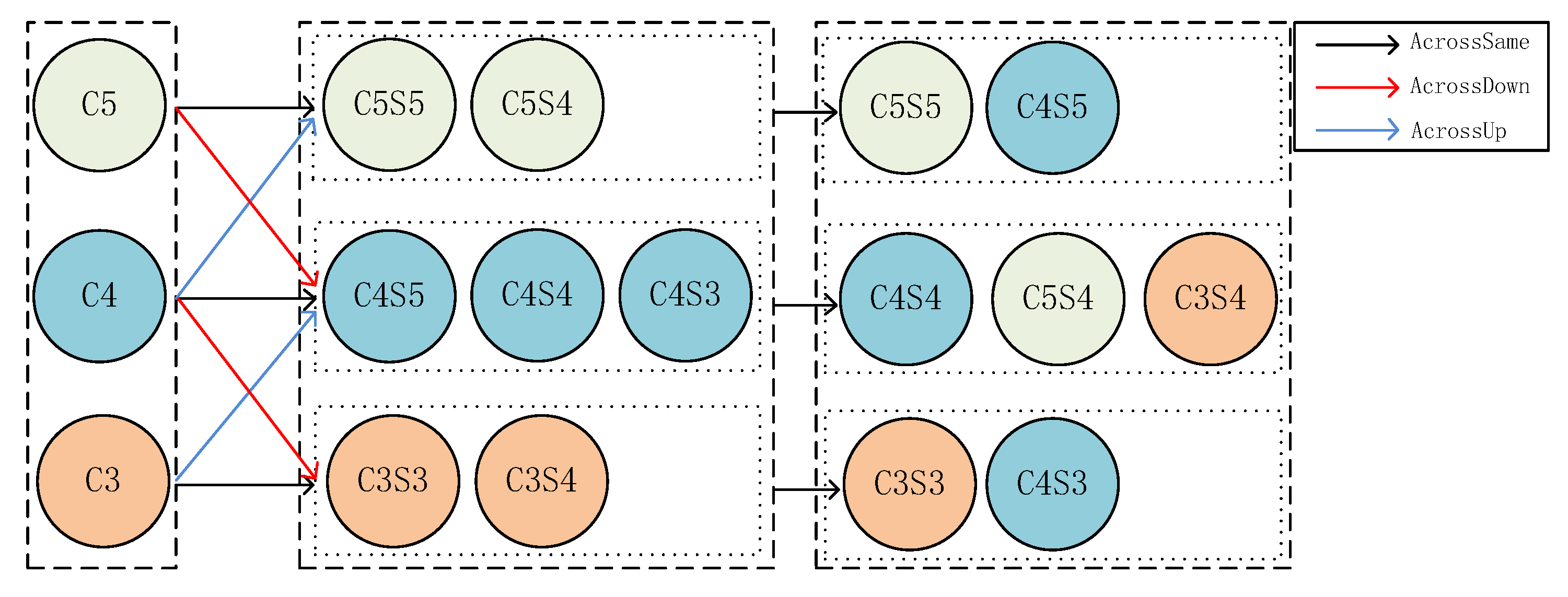
3.2. Feature Constructor

The motivation of the feature constructor module is to exploit the correlation between the adjacent features of the pyramid feature layer to construct a new feature layer so that the new features can alleviate the semantic gap.

First of all, for the feature $F_i(0<i<L-1)\in R^{H\times W}$ where L is the number of FPN layers, three features with sizes $(2H\times 2W,H\times W,H/2\times W/2)$ are generated by $1\times 1$ convolution, $3\times 3$ convolution, and $3\times 3$ convolution whose stride is set to 2, just like feature C4 shown in Figure 2. Then, for the feature $F_0$ and $F_{L-1}$, features of sizes $(2H\times 2W,H\times W)$ and $(H/2\times W/2,H\times W)$ are generated, respectively, referring to C3 and C5 in Figure 2. Finally, features with the same scale are concatenated along the channel dimension to make new feature layers as the output of the module. The new features have both the semantics information of the deep high-level features and the location information of the shallow low-level features. In Figure 2, $S_j$ means the size of the feature layer j. The size of the circle indicates the resolution of the feature.

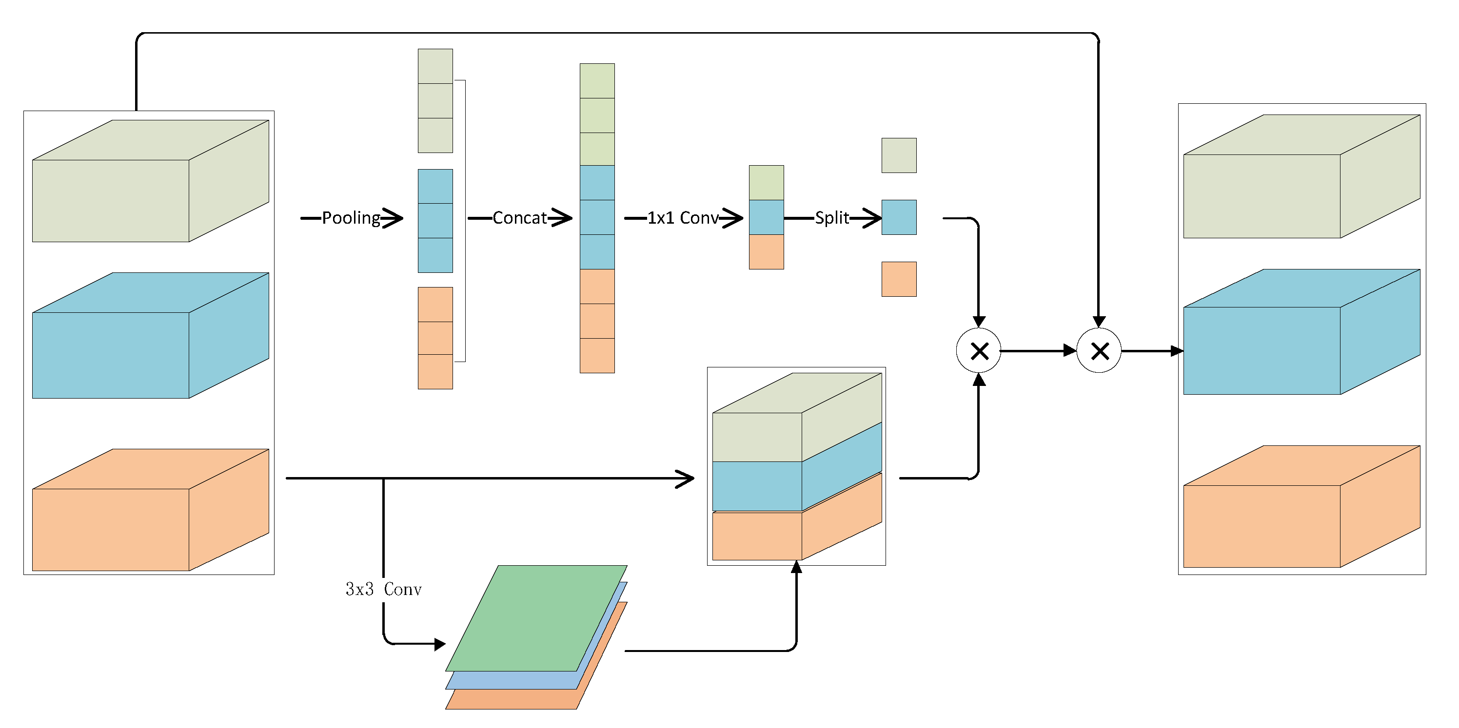
3.3. Multi-Layer Channel and Spatial Attention(MLCS) Module

The main purpose of the multi-layer channel and spatial attention module proposed in this paper is to extract the attention weights from the multi-layer features. As illustrated in Figure 3, the whole multi-layer feature attention module is made up of two parallel branches that extract channel and spatial attention weights from the same data.

The channel attention in MLCS can be calculated according to Formula (1).

$$W_{chn}=\sigma ({Conv}_{1\times 1}\delta ({Conv}_{1\times 1}{Concat}_1^L(\frac{1}{H\times W}\sum _{i,j}^{H,W}{F}_l^{i,j})))$$

(1)

For input multi-layer feature $F\in R^{H\times W\times C\times L}$, a feature of dimension $(1,1,C,L)$ is generated by global average pooling. Then, features of dimension (1, 1, S) are generated by concatenating all features of dimension $(1,1,C)$ along the channel dimension, where we define S as $L\times C$. Finally, linear functions approximated by a $1\times 1$ convolution layer are used to generate the output.

The spatial attention of layer l can be computed as Formula (2).

$$W_{spt}=\sum _{k=1}^K{\omega }_{l,k}·F(l;p_k+\Delta P_k;c)·\Delta m_k$$

(2)

where K is the number of sparse sampling locations, $p_k+\Delta p_k$ is a shifted location to focus on a discriminative region by the self-learned spatial offset $\Delta p_k$, and $\Delta m_k$ is a self-learned importance scalar at location $p_k$. $F_l$ is the feature that concatenates along the channel with dimension $(H,W,S)$.

Finally, the output features of MLCS module can be calculated by Equation (3).

$$F_{out}=F_{in}\odot (W_{chn}\odot W_{spt})$$

(3)

4. Experiments

4.1. Dataset and Evaluation Metrics

All experiments in this paper are performed on the challenging dataset MS COCO-2017 [36]. The dataset contains 80 categories of around 160,000 images (118,000 images for training, 5000 images for validation, and 41,000 images for testing). All reported results follow the standard COCO-style mean Average Precision (mAP) metrics under different Intersection of Union (IOU) thresholds, ranging from 0.5 to 0.95. We also report the results of $A{P}_S$, $A{P}_M$, and $A{P}_L$ on small, medium, and large scales, respectively.

4.2. Implementation Details

For fair comparison, all experiments are implemented with the open source MMDetection [37] toolbox based on Pytorch. We implement CAR as a plugin and train it using the ATSS framework. All other parameters are not noted in this paper following the MMDetection default setting. All models are trained using one compute node of 2 A100 GPUs each with 40 GB memory.

Training. We use ResNet50 as the model backbone in all ablation studies and train it with the standard 1× configuration. Other models are trained with the standard 2× training configurations as introduced in ATSS. Following the typical convention, the long edge and short edge of input images are resized to 1333 and 800. We use stochastic gradient descent (SGD) to train detectors with a batch size of four (two GPUs, two images per GPU) for 12 epochs. The initial learning rate is set to 0.0025 and stepped down by a factor of 10 at eight epochs and 11 epochs.

Inference. We compare our best model with multi-scale testing to state-of-the-art methods reported utilizing test time augmentation. Model EMA, mosaic, mix-up, label smoothing, soft-NMS, and adaptive multi-scale testing are not employed.

4.3. Comparison with State-of-the-Art Detectors

To verify the effectiveness of the BFT, we evaluated the BFT on the MS COCO and compared it with other state-of-the-art detectors. For a fair comparison, we have reimplemented the corresponding baseline methods with FPN on mmdetection.

As shown in

Table 2. Performance comparison with the state-of-the-art (SOTA) results on MS-COCO. Symbol “*” means our reimplemented results, and mark “${}^{†}$” means ResNeXt101-32x4d.

Method	Backbone	Schedule	AP	${\mathit{AP}}_{\mathrm{50}}$	${\mathit{AP}}_{\mathrm{75}}$	${\mathit{AP}}_{\mathit{S}}$	${\mathit{AP}}_{\mathit{M}}$	${\mathit{AP}}_{\mathit{L}}$
anchor-based detector:
ATSS [38]/w FPN *	ResNet50	1×	39.1	57.0	42.5	23.3	42.8	50.1
ATSS [38]/w FPN *	ResNet101	1×	41.5	59.6	45.3	24.9	45.5	53.0
ATSS [38]/w FPN *	ResNet101	2×	41.8	60.2	45.5	25.3	45.9	54.0
YOLOV2 [20]	Darknet19	-	21.6	44.0	19.2	5.0	22.4	35.5
YOLOV3 [22]	Darknet53	-	33.0	57.9	34.4	18.3	35.4	41.9
FreeAnchor [21] *	ResNet50	1×	38.5	57.3	41.2	21.1	41.8	51.5
FreeAnchor [21]/w SEPC *	ResNeXt101 ${}^{†}$	2×	47.7	67.3	51.7	29.2	50.8	60.3
RetinaNet [39]	ResNet101	-	39.1	59.1	42.3	21.8	42.7	50.2
Cascade R-CNN [40]	ResNeXt101	-	42.8	62.1	46.3	23.7	45.5	55.2
Revisiting R-CNN [41]	ResNet101+ResNet152	-	43.1	66.1	47.3	25.8	45.9	55.3
SNIP [1]	DPN-98 [42]	-	45.7	67.3	51.1	29.3	48.8	57.1
Faster R-CNN [19] *	ResNet101	2×	38.7	58.7	42.0	22.1	42.8	50.6
RefineDet512 [43]	ResNet101	-	36.4	57.5	39.5	16.6	39.9	51.4
anchor-free detector:
FoveaBox [44]/w FPN *	ResNet50	1×	36.2	56.1	38.5	20.4	39.7	46.2
FoveaBox [44]/w FPN *	ReNet101	1×	38.3	58.3	40.9	21.4	42.4	50.0
FoveaBox [44]/w FPN *	ReNet101	2×	38.9	58.7	42.0	22.1	42.8	50.6
FCOS [45]	ResNeXt-64x4d-101	2×	43.2	62.8	46.6	26.5	46.2	53.3
RepPoints [46]	ResNeXt101+DCN [47]	-	45.0	66.1	49.0	26.6	48.6	57.5
CenterNet [48]	Hourglass104	-	44.9	62.4	48.1	25.6	47.4	57.4
CornerNet [49]	Hourglass104	-	40.5	56.5	43.1	19.4	42.7	53.9
ours:
ATSS/w BFT	ResNet50	1×	42.8	60.4	46.2	24.1	46.8	57.0
ATSS/w BFT	ResNet101	2×	44.4	61.7	48.1	25.8	49.0	58.6
ATSS/w BFT	ResNeXt101 ${}^{†}$ + DCN [47]	2×	47.3	65.1	51.4	28.4	51.8	62.5
ATSS/w BFT	ResNeXt101 ${}^{†}$ + MDCN [47]	2×	47.8	65.7	52.0	29.0	52.2	63.2
ATSS/w BFT	ResNeXt101-32x4d [6]	2×	47.9	66.2	52.1	28.7	52.8	63.1
ATSS/w BFT	SWIN-T [50]	3×	42.9	60.4	46.9	23.1	47.3	59.2

, when we adopt ResNet50 as the backbone, ATSS with BFT has an improvement of 3.7% over ATSS with FPN, and it has an improvement of 0.8%, 4.0%, and 6.9% for small, medium, and large instances, respectively. The improvement in large-scale objects is quite noticeable. When we adopt ResNet101 as the backbone, ATSS with BFT improves the mAP metric by 2.9% when compared with ATSS with FPN, while ${AP}_s$, ${AP}_m$ and ${AP}_L$ increase by 0.5%, 3.5%, and 5.6%.

When we adopt ResNeXt101 with DCN [47] as the backbone, ATSS with BFT improves the mAP metric by 5.5% when compared to ATSS with FPN while improving various scaled object detection metrics by 3.1%, 5.9%, and 8.8%. It does a better job of detecting little objects, and the overall improvement is more balanced. When we adopt ResNeXt101 with MDCN [47] as the backbone, ATSS with BFT boosts the mAP by 6.0%. For objects of different scales, compared with ATSS with FPN, metrics are improved by 3.7%, 6.3%, and 9.2%.

When adopting ResNeXt101 as the backbone, we also double-check the ATSS with BFT performance under multi-scale training settings. BFT improves the mAP metric to 47.9%, which is a 0.6% improvement over without multi-scale training, while metric $A{P}_{50}$ also improves by 1.1%.

4.4. Ablation Study

4.4.1. Effect of Each Component

In this section, we adopt ResNet50 as the backbone and perform the ablation studies on the MS COCO dataset to analyze the effect of each component in our proposed method by progressively adding additional components to the baseline. We use SGD to train detectors with a batch size of 4 and a learning rate of 0.002 for 12 epochs.

As shown in

Table 3. The results of ablation experiments performed by our algorithm on ATSS and FreeAnchor. [✓] mean the module is added into the pipeline.

Detector	MRFE	Constructor	MLCS	AP	${\mathit{AP}}_{\mathrm{50}}$	${\mathit{AP}}_{\mathrm{70}}$	${\mathit{AP}}_{\mathit{S}}$	${\mathit{AP}}_{\mathit{M}}$	${\mathit{AP}}_{\mathit{L}}$
				39.1	57.0	42.5	23.3	42.8	50.1
	✓			39.1	57.3	42.4	23.5	42.7	51.5
		✓		41.5	58.0	43.0	24.4	43.9	52.7
ATSS			✓	40.3	57.9	43.9	24.2	44.1	51.9
	✓	✓		42.2	59.6	45.6	23.7	46.4	55.8
		✓	✓	42.7	60.1	46.3	25.3	46.8	55.8
	✓		✓	41.6	59.2	44.9	23.9	45.9	54.4
	✓	✓	✓	42.8	60.4	46.2	24.1	46.8	57.0
				38.5	57.3	41.2	21.1	41.8	51.5
	✓			38.2	57.5	41.3	21.4	42.8	52.2
		✓		40.6	58.7	43.5	23.1	44.4	54.6
FreeAnchor			✓	39.9	58.2	42.9	22.5	43.7	53.2
	✓	✓		40.7	58.7	43.5	22.6	44.2	54.6
		✓	✓	41.0	59.2	43.8	22.6	44.7	55.2
	✓		✓	40.3	58.6	43.2	22.7	43.8	53.1
	✓	✓	✓	41.1	59.3	43.8	23.2	44.8	55.0

, after integrating MRFE, feature constructor, and MLCS modules into the ATSS detector, the metric, mAP, increases by 0%, 2.4%, and 1.2%, respectively. The MRFE module can boost the metric ${AP}_L$ by 1.4%, and the feature constructor module makes the highest improvement. In the presence of MRFE and MLCS modules, the feature constructor can still increase the mAP by 1.2%. All the modules together boost the performance of ATSS by about 3.7%.

For the FreeAnchor detector, after integrating the MRFE, feature constructor, and MLCS modules into the detector, separately, the mAP metric increases by −0.3%, 2.1%, and 1.4%. MRFE alone improves the ${AP}_L$ and ${AP}_M$ by 0.7% and 1.0%. The feature constructor is still the module that achieves the highest improvement. The feature constructor in the presence of MRFE and MLCS modules can still improve the performance by 0.8%. All the modules together boost the performance of FreeAnchor by 2.6%.

4.4.2. Effect of Different Baseline

As shown in Table 2, our method achieves 3.7% and 2.6% improvements on ATSS detector and FreeAnchor detector, respectively. By comparing the experimental results, it can be seen that on ATSS, the MRFE module performs poorly on the metric ${AP}_S$, but together with the other two modules, it achieves a huge improvement of 4.0% and 6.9% on ${AP}_M$ and ${AP}_L$. For the detector FreeAnchor, the metrics for detecting large, medium, and small scales objects are improved by 3.5%, 3.0%, and 2.1%, respectively.

From the results shown in Table 2, we can conclude that our method can improve the performance of ATSS detector and FreeAnchor detector with low computational cost. In general, it is believed that our method can be easily plugged into other detectors and improve the performance of the detectors.

4.4.3. Comparison with Other Feature Fusion Modules

In this section, we adopt ResNet50 as the backbone and perform the performance and computational studies on the MS COCO dataset by integrating our method into the FreeAnchor detector. We use SGD to train detectors with a batch size of 4 and a learning rate of 0.002 for 12 epochs.

Table 4. Comparison with other feature fusion modules on FreeAnchor.

Feature Fusion	AP	${\mathit{AP}}_{\mathrm{50}}$	${\mathit{AP}}_{\mathrm{75}}$	FLOPS(G)
FPN	38.5	57.3	41.2	239.3
HRNet	38.6	57.1	41.3	297.6
PANet	38.9	57.6	41.6	245.6
Libra	39.4	58.7	42.2	315.8
NASFPN	39.1	57.0	41.8	347.1
PConv	40.0	59.1	42.2	239.3
BFT	41.1	59.3	43.8	248.7

shows the experimental results.

Table 4 shows that compared with FPN, BFT improves the metric mAP by 2.6% while improving FLOPs by only 3.7%, which is negligible. The detection metric mAP is enhanced by 1.1% when compared to the PConv utilized in SEPC. So, we can conclude that our method can effectively improve the performance of the FreeAnchor detector with low computational cost.

5. Discussion

The definition of feature imbalance in this paper refers to the difference in semantic and location information between feature layers caused by different network depths of feature layers. That is, the high-level features have more semantics than the low-level features. On the contrary, low-level features have more location information than high-level features. The features are situated at various network depths, which is the primary source of the imbalance. However, in order to identify object categories and localize instances, the object detection task requires features with more semantic information and more location information. Another reason is the imbalanced distribution of object categories and scales in the dataset used for training. This article tries to propose a solution to the above reasons.

FPN uses a top–down path to transfer the semantics of high-level features to low-level features in a layer-by-layer fusion manner. PANet transfers the location information of low-level features to high-level features by adding a bottom–up path to the FPN. Due to the sequential fusion manner, the semantic and location information will be attenuated during the transmission process. Another method is to fuse features of different sizes into features of a specific scale, such as the BFP of Libra RCNN, and then directly generate different feature layer sizes through resize. The main idea of this article is to use linear interpolation or convolution functions to directly construct 1/2 and 2×-size features from features on various layers. With the help of the feature construction module, the features of the same scale are constructed into a new feature layer. The new feature consists of the original one and its adjacent features. That is, the new feature has both the semantics of the adjacent high-level features and the location information of the adjacent low-level features. This makes the new features more balanced than those in FPN. The experimental results of ablation show that our method outperforms FPN.

The MLCS module is trained to extract features that are most suitable for the object to be detected. The MLCS module, which is structured in a parallel manner, consists of a channel attention module and a spatial attention module. The motivation is to extract both channel and spatial attention from the same feature, allowing the detector to focus on the specific regions and channel of the feature simultaneously.

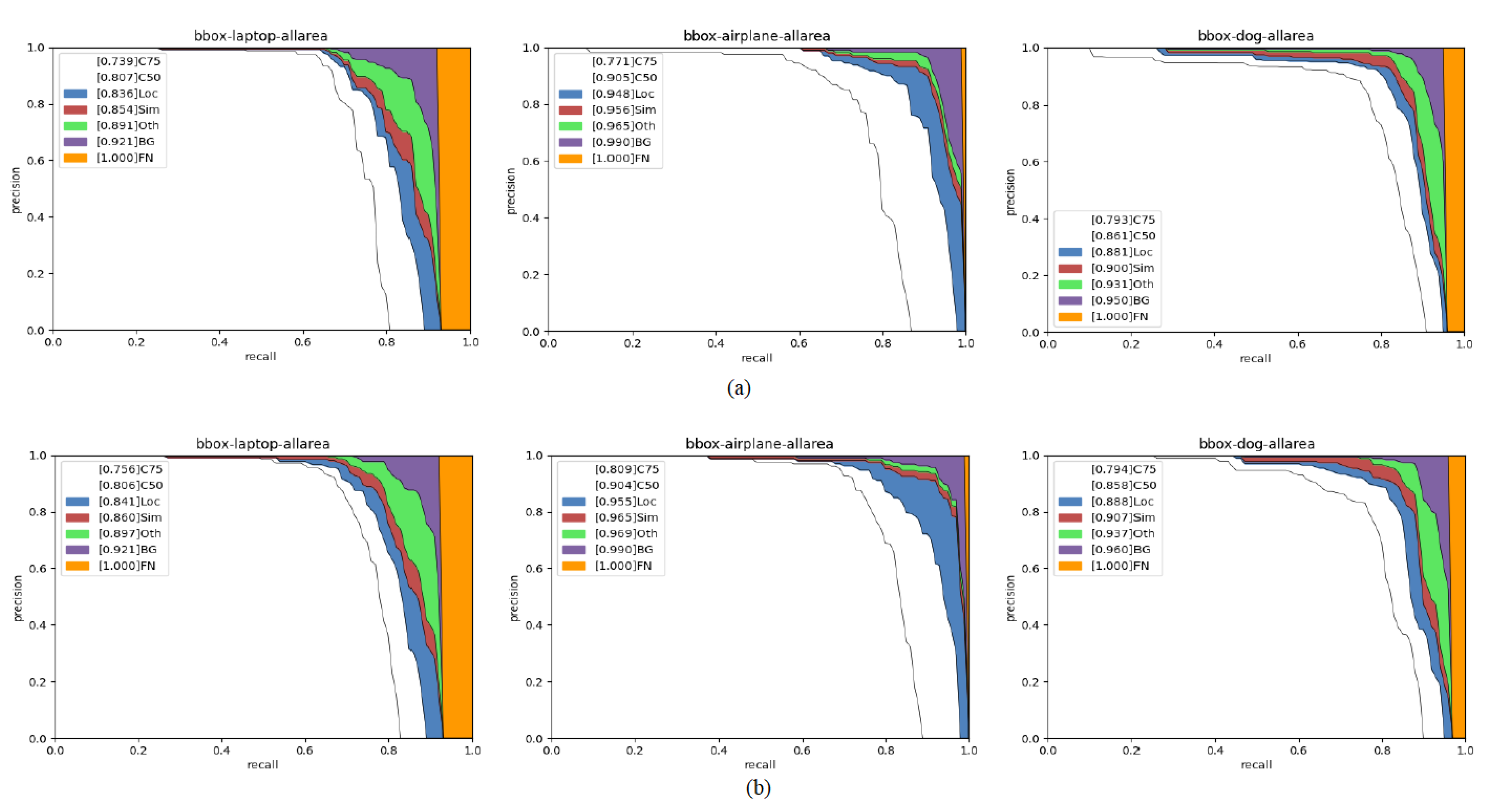
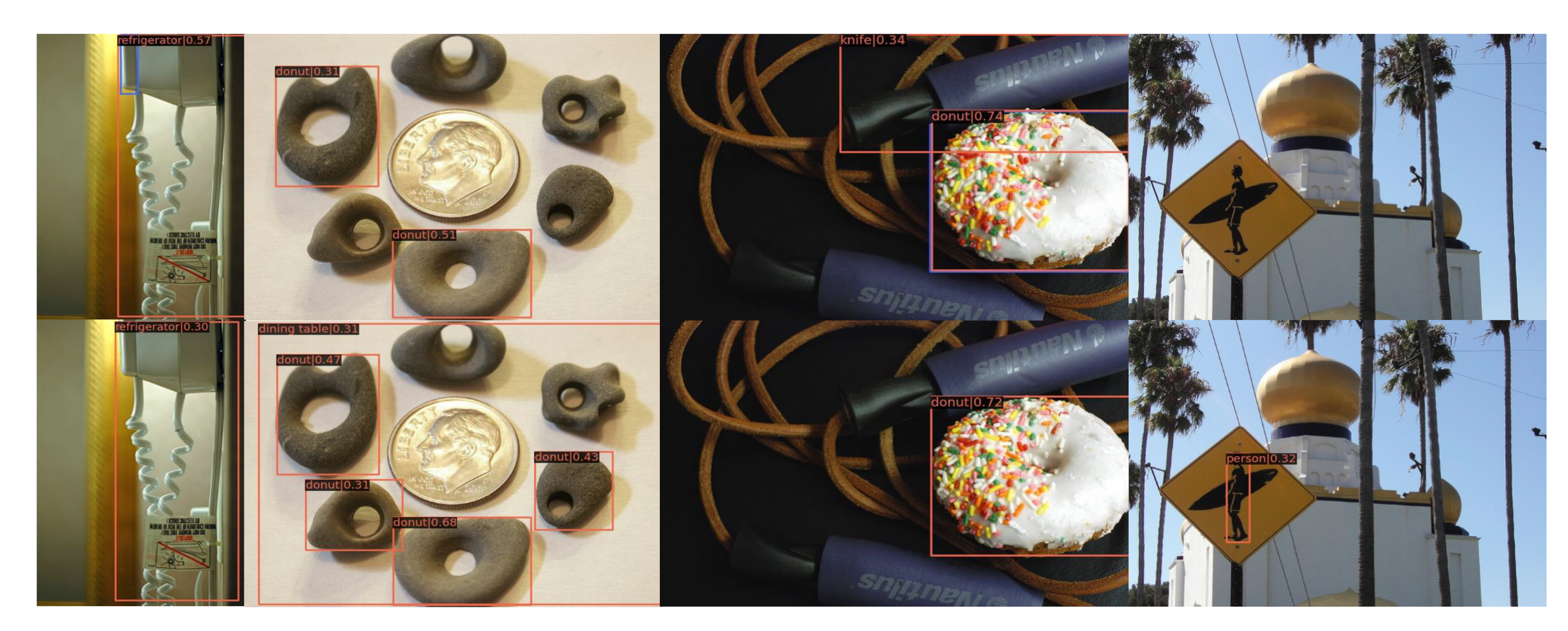
In Figure 4, we compare the ROC of FPN and BFT. In addition, we show the inference output of FPN and BFT in Figure 5. As shown in Figure 4, comparing the ROC results of objects of different sizes, it can be determined that BFT has improved the original algorithm. In Figure 5, we can see that ATSS with BFT can detect more objects and improve the performance of the detector. From Figure 4 and Figure 5, we can conclude that BFT can boost the performance of the detector over FPN.

The results of the ablation experiments in Table 3 show that MRFE plays a limited role in the whole pipeline, and the core module is the feature constructor block and the MLCS block. In the ablation experiment, we verify the effect of each module by gradually adding each module to the pipeline, and we also verify the effect of the combination of two modules on the experimental results. From the experimental results, it can be concluded that the performance of the baseline has been improved, and each module works well.

We show the performance and computational cost comparisons with other feature fusion methods in Table 4. When compared to FPN, BFT improves the performance by 2.6% while only increasing the computing costs by 3.7%. From the experimental results, it can be concluded that BFT is a low-cost fusion method and an effective method.

We integrate BFT into ATSS and show the results in Table 2 after comparing it with other SOTA detectors. We conduct experiments on different backbones, such as ResNet and ResNeXt, with or without DCN. The results show that the overall detector performance can be improved by embedding our method into the network.

We have verified that our method can improve the detection performance of the network, but in fact, there is still no way to quantitatively measure the specific difference in semantics and positioning information between the feature layers. Although it is possible to use training loss or IOU loss, as well as positive and negative sample ratios, etc., those methods require relatively complex calculations. We are exploring a new way to directly measure the imbalance of features. This is also our later work.

6. Conclusions

In this paper, we discuss the feature imbalance problem and propose a reconstructive approach, combined with the MLCS attention method, to effectively improve the detection performance of the network. The BFT method can be integrated into the pipeline to alleviate the output feature imbalance. Based on the experimental results shown in the paper, we believe that BFT can alleviate network feature imbalance.

During the experiment in this paper, we found that using different attention algorithms on features of different depths will affect the experimental results of the algorithm. This paper only proposes a network structure and a simple multi-feature layer attention algorithm. In the future, we will shift our attention to the adaptive attention algorithm, which can automatically calculate the attention weights of different depths of features.

References

- Singh, B.; Davis, L.S. An analysis of scale invariance in object detection snip. In Proceedings of the IEEE Conference on Computer Vision and Pattern Recognition, Salt Lake City, UT, USA, 18–23 June 2018; pp. 3578–3587. [Google Scholar]
- Singh, B.; Najibi, M.; Davis, L.S. Sniper: Efficient multi-scale training. Adv. Neural Inf. Process. Syst. 2018, 31, 9333–9334. [Google Scholar]
- Gepreel, K.A.; Higazy, M.; Mahdy, A. Optimal control, signal flow graph, and system electronic circuit realization for nonlinear Anopheles mosquito model. Int. J. Mod. Phys. C (IJMPC) 2020, 31, 2050130. [Google Scholar] [CrossRef]
- Lin, T.Y.; Dollár, P.; Girshick, R.; He, K.; Hariharan, B.; Belongie, S. Feature pyramid networks for object detection. In Proceedings of the IEEE Conference on Computer Vision and Pattern Recognition, Salt Lake City, UT, USA, 18–23 June 2018; pp. 2117–2125. [Google Scholar]
- He, K.; Zhang, X.; Ren, S.; Sun, J. Deep residual learning for image recognition. In Proceedings of the IEEE Conference on Computer Vision and Pattern Recognition, Las Vegas, NV, USA, 27–30 June 2016; pp. 770–778. [Google Scholar]
- Xie, S.; Girshick, R.; Dollár, P.; Tu, Z.; He, K. Aggregated residual transformations for deep neural networks. In Proceedings of the IEEE Conference on Computer Vision and Pattern Recognition, Salt Lake City, UT, USA, 18–23 June 2018; pp. 1492–1500. [Google Scholar]
- Tan, M.; Pang, R.; Le, Q.V. Efficientdet: Scalable and efficient object detection. In Proceedings of the IEEE/CVF Conference on Computer Vision and Pattern Recognition, Seattle, WA, USA, 13–19 June 2020; pp. 10781–10790. [Google Scholar]
- Chen, K.; Cao, Y.; Loy, C.C.; Lin, D.; Feichtenhofer, C. Feature pyramid grids. arXiv 2020, arXiv:2004.03580. [Google Scholar]
- Gong, Y.; Yu, X.; Ding, Y.; Peng, X.; Zhao, J.; Han, Z. Effective fusion factor in FPN for tiny object detection. In Proceedings of the IEEE/CVF Winter Conference on Applications of Computer Vision, Online, 5–9 January 2021; pp. 1160–1168. [Google Scholar]
- Newell, A.; Yang, K.; Deng, J. Stacked hourglass networks for human pose estimation. In Proceedings of the European Conference on Computer Vision, Amsterdam, The Netherlands, 8–16 October 2016; pp. 483–499. [Google Scholar]
- Wang, J.; Sun, K.; Cheng, T.; Jiang, B.; Deng, C.; Zhao, Y.; Liu, D.; Mu, Y.; Tan, M.; Wang, X.; et al. Deep high-resolution representation learning for visual recognition. IEEE Trans. Pattern Anal. Mach. Intell. 2020, 43, 3349–3364. [Google Scholar] [CrossRef] [PubMed]
- Liu, S.; Qi, L.; Qin, H.; Shi, J.; Jia, J. Path aggregation network for instance segmentation. In Proceedings of the IEEE Conference on Computer Vision and Pattern Recognition, Salt Lake City, UT, USA, 18–23 June 2018; pp. 8759–8768. [Google Scholar]
- Pang, J.; Chen, K.; Shi, J.; Feng, H.; Ouyang, W.; Lin, D. Libra r-cnn: Towards balanced learning for object detection. In Proceedings of the IEEE/CVF Conference on Computer Vision and Pattern Recognition, Long Beach, CA, USA, 15–20 June 2019; pp. 821–830. [Google Scholar]
- Wang, X.; Zhang, S.; Yu, Z.; Feng, L.; Zhang, W. Scale-equalizing pyramid convolution for object detection. In Proceedings of the IEEE/CVF Conference on Computer Vision and Pattern Recognition, Seattle, WA, USA, 13–19 June 2020; pp. 13359–13368. [Google Scholar]
- Zhang, Y.; Wang, C.; Wang, X.; Zeng, W.; Liu, W. FairMOT: On the Fairness of Detection and Re-identification in Multiple Object Tracking. Int. J. Comput. Vis. 2021, 129, 3069–3087. [Google Scholar] [CrossRef]
- Feng, D.; Haase-Schutz, C.; Rosenbaum, L.; Hertlein, H.; Dietmayer, K. Deep Multi-Modal Object Detection and Semantic Segmentation for Autonomous Driving: Datasets, Methods, and Challenges. IEEE Trans. Intell. Transp. Syst. 2020, 22, 1341–1360. [Google Scholar] [CrossRef]
- Karaoguz, H.; Jensfelt, P. Object Detection Approach for Robot Grasp Detection. In Proceedings of the 2019 International Conference on Robotics and Automation (ICRA), Montreal, QC, Canada, 20–24 May 2019. [Google Scholar]
- Jaeger, P.F.; Kohl, S.A.A.; Bickelhaupt, S.; Isensee, F.; Kuder, T.A.; Schlemmer, H.P.; Maier-Hein, K.H. Retina U-Net: Embarrassingly Simple Exploitation of Segmentation Supervision for Medical Object Detection. In Proceedings of the Machine Learning for Health Workshop, Cambridge, MA, USA, 10 March 2020; pp. 171–183. [Google Scholar]
- Ren, S.; He, K.; Girshick, R.; Sun, J. Faster r-cnn: Towards real-time object detection with region proposal networks. Adv. Neural Inf. Process. Syst. 2015, 28, 1137–1149. [Google Scholar] [CrossRef] [PubMed]
- Redmon, J.; Farhadi, A. YOLO9000: Better, faster, stronger. In Proceedings of the IEEE Conference on Computer Vision and Pattern Recognition, Salt Lake City, UT, USA, 18–23 June 2018; pp. 7263–7271. [Google Scholar]
- Zhang, X.; Wan, F.; Liu, C.; Ji, R.; Ye, Q. Freeanchor: Learning to match anchors for visual object detection. Adv. Neural Inf. Process. Syst. 2019, 7, 32–45. [Google Scholar]
- Redmon, J.; Farhadi, A. Yolov3: An incremental improvement. arXiv 2018, arXiv:1804.02767. [Google Scholar]
- Bochkovskiy, A.; Wang, C.Y.; Liao, H.Y.M. Yolov4: Optimal speed and accuracy of object detection. arXiv 2020, arXiv:2004.10934. [Google Scholar]
- Liu, S.; Huang, D. Receptive field block net for accurate and fast object detection. In Proceedings of the European Conference on Computer Vision (ECCV), Munich, Germany, 8–14 September 2018; pp. 385–400. [Google Scholar]
- Chen, L.C.; Zhu, Y.; Papandreou, G.; Schroff, F.; Adam, H. Encoder-decoder with atrous separable convolution for semantic image segmentation. In Proceedings of the European Conference on Computer Vision (ECCV), Munich, Germany, 8–14 September 2018; pp. 801–818. [Google Scholar]
- Ding, X.; Zhang, X.; Ma, N.; Han, J.; Ding, G.; Sun, J. Repvgg: Making vgg-style convnets great again. In Proceedings of the IEEE/CVF Conference on Computer Vision and Pattern Recognition, Online, 20–25 June 2021; pp. 13733–13742. [Google Scholar]
- Howard, A.G.; Zhu, M.; Chen, B.; Kalenichenko, D.; Wang, W.; Weyand, T.; Andreetto, M.; Adam, H. Mobilenets: Efficient convolutional neural networks for mobile vision applications. arXiv 2017, arXiv:1704.04861. [Google Scholar]
- Guo, C.; Fan, B.; Zhang, Q.; Xiang, S.; Pan, C. Augfpn: Improving multi-scale feature learning for object detection. In Proceedings of the IEEE/CVF Conference on Computer Vision and Pattern Recognition, Seattle, WA, USA, 13–19 June 2020; pp. 12595–12604. [Google Scholar]
- Luo, Y.; Cao, X.; Zhang, J.; Guo, J.; Shen, H.; Wang, T.; Feng, Q. CE-FPN: Enhancing channel information for object detection. Multimed. Tools Appl. 2022, 13, 1–20. [Google Scholar] [CrossRef]
- Wang, X.; Girshick, R.; Gupta, A.; He, K. Non-local neural networks. In Proceedings of the IEEE Conference on Computer Vision and Pattern Recognition, Salt Lake City, UT, USA, 18–23 June 2018; pp. 7794–7803. [Google Scholar]
- Ghiasi, G.; Lin, T.Y.; Le, Q.V. Nas-fpn: Learning scalable feature pyramid architecture for object detection. In Proceedings of the IEEE/CVF Conference on Computer Vision and Pattern Recognition, Long Beach, CA, USA, 15–20 June 2019; pp. 7036–7045. [Google Scholar]
- Liu, S.; Huang, D.; Wang, Y. Learning spatial fusion for single-shot object detection. arXiv 2019, arXiv:1911.09516. [Google Scholar]
- Luo, W.; Li, Y.; Urtasun, R.; Zemel, R. Understanding the effective receptive field in deep convolutional neural networks. Adv. Neural Inf. Process. Syst. 2016, 29, 4905–4913. [Google Scholar]
- Dai, J.; Li, Y.; He, K.; Sun, J. R-fcn: Object detection via region-based fully convolutional networks. Adv. Neural Inf. Process. Syst. 2016, 29, 379–387. [Google Scholar]
- Dai, Y.; Gieseke, F.; Oehmcke, S.; Wu, Y.; Barnard, K. Attentional feature fusion. In Proceedings of the IEEE/CVF Winter Conference on Applications of Computer Vision, Online, 5–9 January 2021; pp. 3560–3569. [Google Scholar]
- Lin, T.Y.; Maire, M.; Belongie, S.; Hays, J.; Perona, P.; Ramanan, D.; Dollár, P.; Zitnick, C.L. Microsoft coco: Common objects in context. In Proceedings of the European Conference on Computer Vision, Zurich, Switzerland, 6–12 September 2014; pp. 740–755. [Google Scholar]
- Chen, K.; Wang, J.; Pang, J.; Cao, Y.; Xiong, Y.; Li, X.; Sun, S.; Feng, W.; Liu, Z.; Xu, J.; et al. MMDetection: Open mmlab detection toolbox and benchmark. arXiv 2019, arXiv:1906.07155. [Google Scholar]
- Zhang, S.; Chi, C.; Yao, Y.; Lei, Z.; Li, S.Z. Bridging the gap between anchor-based and anchor-free detection via adaptive training sample selection. In Proceedings of the IEEE/CVF Conference on Computer Vision and Pattern Recognition, Seattle, WA, USA, 13–19 June 2020; pp. 9759–9768. [Google Scholar]
- Lin, T.Y.; Goyal, P.; Girshick, R.; He, K.; Dollár, P. Focal loss for dense object detection. In Proceedings of the IEEE International Conference on Computer Vision, Venice, Italy, 22–29 October 2017; pp. 2980–2988. [Google Scholar]
- Cai, Z.; Vasconcelos, N. Cascade r-cnn: Delving into high quality object detection. In Proceedings of the IEEE Conference on Computer Vision and Pattern Recognition, Salt Lake City, UT, USA, 18–23 June 2018; pp. 6154–6162. [Google Scholar]
- Cheng, B.; Wei, Y.; Shi, H.; Feris, R.; Xiong, J.; Huang, T. Revisiting rcnn: On awakening the classification power of faster rcnn. In Proceedings of the European Conference on Computer Vision (ECCV), Munich, Germany, 8–14 September 2018; pp. 453–468. [Google Scholar]
- Chen, Y.; Li, J.; Xiao, H.; Jin, X.; Yan, S.; Feng, J. Dual path networks. Adv. Neural Inf. Process. Syst. 2017, 30, 4470–4478. [Google Scholar]
- Zhang, S.; Wen, L.; Bian, X.; Lei, Z.; Li, S.Z. Single-shot refinement neural network for object detection. In Proceedings of the IEEE Conference on Computer Vision and Pattern Recognition, Salt Lake City, UT, USA, 18–23 June 2018; pp. 4203–4212. [Google Scholar]
- Kong, T.; Sun, F.; Liu, H.; Jiang, Y.; Li, L.; Shi, J. Foveabox: Beyound anchor-based object detection. IEEE Trans. Image Process. 2020, 29, 7389–7398. [Google Scholar] [CrossRef]
- Tian, Z.; Shen, C.; Chen, H.; He, T. Fcos: Fully convolutional one-stage object detection. In Proceedings of the IEEE/CVF International Conference on Computer Vision, Seoul, Korea, 27 October–2 November 2019; pp. 9627–9636. [Google Scholar]
- Yang, Z.; Liu, S.; Hu, H.; Wang, L.; Lin, S. Reppoints: Point set representation for object detection. In Proceedings of the IEEE/CVF International Conference on Computer Vision, Seoul, Korea, 27 October–2 November 2019; pp. 9657–9666. [Google Scholar]
- Dai, J.; Qi, H.; Xiong, Y.; Li, Y.; Zhang, G.; Hu, H.; Wei, Y. Deformable convolutional networks. In Proceedings of the IEEE International Conference on Computer Vision, Venice, Italy, 22–29 October 2017; pp. 764–773. [Google Scholar]
- Duan, K.; Bai, S.; Xie, L.; Qi, H.; Huang, Q.; Tian, Q. Centernet: Keypoint triplets for object detection. In Proceedings of the IEEE/CVF International Conference on Computer Vision, Seoul, Korea, 27 October–2 November 2019; pp. 6569–6578. [Google Scholar]
- Law, H.; Deng, J. Cornernet: Detecting objects as paired keypoints. In Proceedings of the European Conference on Computer Vision (ECCV), Munich Germany, 8–14 September 2018; pp. 734–750. [Google Scholar]
- Liu, Z.; Lin, Y.; Cao, Y.; Hu, H.; Wei, Y.; Zhang, Z.; Lin, S.; Guo, B. Swin transformer: Hierarchical vision transformer using shifted windows. In Proceedings of the IEEE/CVF International Conference on Computer Vision, Online, 11–17 October 2021; pp. 10012–10022. [Google Scholar]