Abstract
This research proposes a methodology for the selection of input variables based on eXplainable AI (XAI) for energy consumption prediction. For this purpose, the energy consumption prediction model (R2 = 0.871; MAE = 2.176; MSE = 9.870) was selected by collecting the energy data used in the building of a university in Seoul, Republic of Korea. Applying XAI to the results from the prediction model, input variables were divided into three groups by the expectation of the ranking-score () (10 ≤ Strong, 5 ≤ Ambiguous < 10, and Weak < 5), according to their influence. As a result, the models considering the input variables of the Strong + Ambiguous group (R2 = 0.917; MAE = 1.859; MSE = 6.639) or the Strong group (R2 = 0.916; MAE = 1.816; MSE = 6.663) showed higher prediction results than other cases (p < 0.05 or 0.01). There were no statistically significant results between the Strong group and the Strong + Ambiguous group (R2: p = 0.408; MAE: p = 0.488; MSE: p = 0.478). This means that when considering the input variables of the Strong group (: Year = 14.8; E-Diff = 12.8; Hour = 11.0; Temp = 11.0; Surface-Temp = 10.4) determined by the XAI-based methodology, the energy consumption prediction model showed excellent performance. Therefore, the methodology proposed in this study is expected to determine a model that can accurately and efficiently predict energy consumption.
1. Introduction
As environmental problems arise due to global warming, greenhouse gas emissions have emerged as a serious problem [1]. In 2005, the Kyoto Protocol went into effect, and the reduction of greenhouse gas emissions began to be made mandatory in developed countries; while in 2014, the Intergovernmental Panel on Climate Change recommended the high-level reduction of greenhouse gas emissions [2,3]. To efficiently manage such greenhouse gas emissions, it is necessary to balance energy consumption and supply [4]; in addition, sophisticated prediction research on energy consumption is required in advance [5]. Accurately predicting energy consumption is an important strategy for improving energy efficiency [6], and it occupies an important part in low-carbon energy conversion and renewable energy projects [7,8].
For this purpose, various studies on energy consumption prediction based on machine learning or deep learning were recently conducted. Fang and Lahdelma (2016) used the SARIMA model to predict heat demand and reported the prediction accuracy of (91, 77, and 96) % R2 values for the overall, summer, and winter seasons, respectively. The input variables used for this purpose were outdoor temperature, wind speed, weekly and daily usage patterns, and regional information (residential, commercial, and industrial areas) [9]. Sandberg et al. (2017) predicted actual heat demand data using eight weather information, holiday information, heat demand from the previous day (kWh), heat demand from the same time period one week ago (kWh), and average heat demand for the past 24 h (kWh) [10]. Johanson et al. (2017) presented an online machine learning prediction algorithm based on Extra-Trees Regressor and Extreme Learning Machines, and the input variables used in this case were actual weather forecast and historical heat demand data [11]. However, other than on the training data, their model showed somewhat poor performance under exceptional circumstances.
As mentioned above, although various studies on energy demand forecasting were conducted, there were differences in the input variables used depending on the purpose. To predict the heating energy demand of a residential building, solar radiation, wind speed, external temperature, hot water flow rate the previous day, and facility outlet hot water temperature were used as input variables [12]. Additionally, the history of building use, the characteristics of heating power, and climate data were considered to predict the heating demand in a short time range [13]. In a study to predict the energy consumption used in schools, information on the school’s architectural form and architectural characteristics were adopted as input variables [14]. Magalhaes et al. (2017) used building characteristics and location information, heating patterns, and indoor temperature as input variables in their study to specify the relationship between heating patterns and energy demand [15]. However, to the best of our knowledge, the criteria or rationale for the selection of input variables were not clearly presented.
This study proposes a novel methodology for the selection of input variables for forecasting energy consumption based on eXplainable artificial intelligence (XAI). Developed to solve the “Black-box” problem of the AI model, XAI is another artificial intelligence (AI) model that makes it possible to explain the results derived from other AI models and their processes [16]. The XAI is a state-of-the-art algorithm that enables the analysis of reliability, evidence, error causes, and improvement plans of results derived from artificial intelligence models [17]. In this study, these characteristics of XAI are applied to analyze the influence of input variables on energy consumption forecasting and, through this, select an optimal input variable.
2. Materials and Methods
2.1. Overview
Figure 1 shows the overall workflow for the XAI-based input variable selection methodology for energy consumption forecasting. First, a model for energy consumption forecasting was determined using directly measured energy consumption data and input variables selected through literature research. XAI was applied to the results derived from the determined model, and three groups (Strong, Ambiguous, and Weak) were classified with the magnitude of the influence of each input variable on the prediction result. Finally, the optimal input variables were selected by re-evaluating the energy consumption forecasting model selected for each group and intergroup combination.
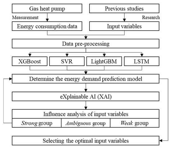
Figure 1.
Overall workflow for XAI-based input variable selection for energy consumption forecasting.
2.2. Data Acquisition
2.2.1. Target Variable: Energy Consumption Data
The actual energy consumption data were measured from a gas heat pump (GHP) installed in a university building in Seoul, Korea of Republic, to learn the energy consumption forecasting model. The building is a complex with a total of 17 floors (5 basement floors and 12 ground floors): Parking lot from the 5th basement floor to the 3rd basement floor; classrooms on the 2nd and 1st basement floors; convenience facilities, such as hospitals, pharmacies, cafes, and restaurants, on the 1st and 2nd floors; venture companies and meeting rooms on the 3rd floor; professorial laboratories and graduate school laboratories on the 4th to 8th floors; guesthouses on the 9th to 11th floors; and 12th floor conference room. The actual measurement period of energy consumption data was from 14:00 on 15 December 2020, to 13:00 on 15 December 2021, and a total of 8760 data were acquired for each time.
2.2.2. Input Variables: Time Information, Climate Data, and Historical Energy Consumption Data
The input variables used to build the energy consumption prediction model consist of time information, climate data, and past energy consumption data, which were selected through previous research in the literature (Table 1). The climate data were acquired in XML format through the open API of the Automated Surface Observing System, and the energy consumption data measured were used for the historical energy data.

Table 1.
Input variables selected to build the energy consumption forecasting model.
2.3. Energy Consumption Forecasting Models
All models used to forecast energy consumption were evaluated by classifying data into 80% training dataset, 10% validation dataset, and 10% test dataset, which were randomly selected. In order to maintain data integrity, null values were replaced with the average of the before and after values, and categorical variables were converted into numeric variables. The numeric input variables used in all models were normalized within the range of 0 and 1. Additionally, zero values were replaced with a very small value (10−6) to improve the forecasting performance.
Extreme Gradient Boosting (XGBoost) is a distributed gradient-boosted decision tree machine learning library for solving classification and regression problems [27], and in this study, a Classification and regression tree (CART) [28] was used. Regression and mean absolute error (MAE) were used for the objective function and loss function, respectively. The hyperparameters are used to minimize a value of the mlogloss, which is an evaluation index of a training set. The eta that represents a learning rate was 0.05, the gamma for specifying loss reduction was 0, the max_depth that represents the maximum depth of an ensemble model tree was 5. The min_child_weight to adjust the minimum value of the sum of weights for the observed values was 1.
Support vector regression (SVR) is a regression analysis algorithm derived from the support vector machine (SVM), which is widely used in the classification, regression, and outlier discrimination fields [29] and was used to predict energy consumption in this study. The thickness E of a tube is 0.5. The SVR uses the loss function, which does not penalize’ errors below some E (> 0). The penalty factor C, which penalizes any deviation beyond the ϵ-tube, is 1. The gaussian radial basis function is considered, so the gamma was set automatically.
The Light Gradient Boosting Model (LightGBM) is a horizontal tree learning algorithm based on gradient boosting, and consists of gradient-based one-side sampling (GOSS) and greedy bundling [30]. The GOSS was used to extract samples for the energy consumption forecasting model, and greedy bundling was used to select features to ensure the performance of the model [30]. The maximum depth (max_depth) of the tree was −1. The num_leaves for searching the maximum tree leaves for base learners was 31. The learning rate was 0.01, and finally, boosting as the gbdt-gradient boosting decision tree.
Long short-term memory (LSTM) is a neural network structure developed to solve the long-term dependencies of recurrent neural networks (RNNs) and is mainly used to forecast long-term time-series data, such as energy consumption [31,32,33]. The number of hidden layers was 2, and the number of hidden layer neurons was 128. The tanh function was used to prevent the loss of the model, and the sigmoid function was used at the output layer for interpreting. Mean squared error (MSE) was chosen as the loss function to calculate the error for predicting and target values. The adam algorithm was used as a model optimizer. Epochs were set to 50, and batch size was 16.
Coefficient of determination (R2) [34], mean absolute error (MAE) [35], and mean squared error (MSE) [36] were used to evaluate and compare the performance of energy consumption forecasting models. The R2 was used to compare the scale of the actual value with the predicted value by the models used for energy consumption forecasting in this study, while MAE and MSE, which are mainly used for regression problems, were used to quantify the error between the actual and predicted energy consumptions. The best energy consumption forecasting model was selected through the results calculated by these performance indicators. Using the model, a total of 10 models were constructed, from a model using data from the previous day as an input variable, to a model using accumulated data for 10 days.
2.4. Selection of Optimal Variables Based on eXplainable AI (XAI) for Energy Consumption Forecasting
The Shapley additive explanation (SHAP) of XAI was applied to all results derived from the 10 models to quantitatively analyze the influence of input variables on the energy consumption forecasting results. XAI is a state-of-the-art technology to find answers about how much to trust the results derived from the artificial intelligence model, what is the reason for the derivation, and how to improve the model [17]. The SHAP is a technique that calculates the contribution of each input variable to the prediction result using Shapley values [37,38]. The XAI regenerated 215 = 32,768 models for each forecasting model, where 15 represents the number of input variables, and calculated the difference in prediction results according to the presence or absence of all input variables, to obtain the importance of specific variables. This process was repeated for the 10 models.
The 15 input variables were classified into three groups (Strong, Ambiguous, and Weak) by analyzing the results of XAI applied to the energy consumption forecasting model. For this, a ranking-score was assigned to each input variable: {1st = 15; 2nd = 14; …; 14th = 2; 15th = 1}, and was quantified as the expectation of the score (Equation (1)):
where means the expectation of the ranking-score of the input variable, and and represent the number of days of analysis of (1–10 days) and the -th ranking-score of the variable, respectively. is the probability of occurrence of , and 0.1 was used here. Therefore, the minimum value of was 1, while the maximum was 15. was classified into Strong, Ambiguous, and Weak groups according to Equation (2):
The optimal input variables were determined by re-evaluating the consumption forecasting models for each group and intergroup combination (Strong + Ambiguous, Strong + Weak, Ambiguous + Weak, and Strong + Ambiguous + Weak).
2.5. Statiatical Analysis
The difference between the energy consumption forecasting results for each group and the intergroup combination was analyzed using independent t-test. For statistical analysis, SPSS 15.0 software (SPSS Inc., Chicago, IL, USA) was used, and all statistical significance levels were 0.05 or 0.01.
3. Results
3.1. Energy Consumption Data
The energy consumption data measured from the city gas meter (gas, heat pump, GHP) consist of the uncorrected cumulative value, the correction coefficient and the compression coefficient, and the temperature and pressure values of the gas at the moment it passes through the meter. The uncorrected cumulative value means the pure value before the standard condition measured by the mechanical meter. The energy consumption data used in this study were the corrected cumulative value obtained by converting the uncorrected cumulative value with the correction and compression factors. Figure 2 shows the corrected cumulative values for each hour measured from 14:00 on 15 December 2020, to 13:00 on 15 December 2021.

Figure 2.
Changes in energy consumption data measured from GHP for (a) hour, (b) day, and (c) month.
The x- and y-axes represent time and energy consumption, respectively, and the unit of energy consumption is the normal cubic meter per hour. The energy consumption data showed a tendency to increase in the summer and winter seasons due to cooling and heating, respectively, and to decrease in the spring and autumn seasons. According to the report from the National Weather Service [39], the cooling-related energy consumption increases in summer due to the hot and humid characteristics of the domestic weather, while winter is generally cold and dry under the influence of continental cyclones, increasing heating-related energy consumption. In spring and fall, energy consumption is low due to the clear and dry days caused by migratory anticyclones.
3.2. Results of Energy Consumption Forecasting Models
Figure 3 shows the prediction results of four models on the test data (red solid line). The x-axis and y-axis represent the number of test data and the energy consumption , respectively. Figure 3a–d show the energy consumption results for each model on test data, respectively.

Figure 3.
Energy consumption prediction results for each model on test data. (a) XGBoost, (b) SVR, (c) LightGBM, and (d) LSTM.
Table 2 shows the performance evaluation results of each model for the test data. In R2, LSTM showed the highest level, and MAE and MSE were lowest in LightGBM and LSTM, respectively. The predictive model that showed the lowest overall performance evaluation was SVR. In this study, the best energy consumption forecasting model was preferentially selected with the highest coefficient of determination (R2 = 0.871). Therefore, the LSTM model was determined even though the MAE was not the first priority. The LSTM model establishment was implemented using Tensorflow with version 1.14.0 and Keras 2.2.4 and Python 3.7.13 (64-bit). It took 19 min and 24 s for the model to learn the data and approximately 30 s for prediction.
Table 2.
Performance evaluation result of each forecasting model on test data.
Table 3 shows the performance evaluation results for forecasting energy consumption by applying the 15 input variables to the LSTM model from (1 to 10 days). The range of R2 was (0.705–0.912), and the ranges of MAE and MSE were (1.966–4.143) and (6.963–16.855), respectively. The model using 2 days (48 h) of data showed the highest R2 value (0.912), while the 1-day (24 h) data-based model showed the lowest error. There was no significant trend for each period.
Table 3.
LSTM energy consumption forecasting performance for time (1 to 10 days).
3.3. Optimal Input Variables by Using XAI (SHAP)
The XAI (SHAP) was applied to interpret the influence of input variables on the predicted energy consumption results for each time period, and Figure 4 shows a sample of the results, i.e., a sample of the SHAP value for the predicted result using 6 days of data. The vertical axis represents the 15 input variables considered in this study, and the horizontal axis is the impact on model output. The SHAP values are expressed in the form of dots with the influence of each input variable. Each input variable means a positive influence on the right side and a negative on the left side on the prediction result centered on the baseline (SHAP value = 0.00). The range of the SHAP value indicates the degree of influence on the prediction result, and through this, the variables located on the vertical axis are sorted in order of importance from top to bottom. In this case, it was found that the Year had the largest influence on the prediction result, while the S-I-amount had the smallest influence.

Figure 4.
Sample of XAI analysis results for the 6 days (144 h) data-based energy consumption forecasting model.
The expected value of the ranking-score calculated by Equation (1) was classified into three groups according to the criterion of Equation (2), and the results were represented with the value of (Table 4).
Table 4.
Input variable grouping according to the XAI analysis results.
3.4. Performance Evaluation with The Optimal Variables
Figure 5 shows the results of energy consumption predicted by applying each group and intergroup combination to the LSTM model. Figure 5a–c shows the performance of the LSTM model evaluated by R2, MAE, and MSE, respectively, and the differences between each group were analyzed statistically. The higher the R2, the lower the MAE and MSE, the better the predictive performance, and each evaluation index was presented in order of the highest performance. The groups containing Strong showed high R2 and low MAE and MSE, while in contrast, the groups containing Weak showed low performance. In all the results, the predictive performances of the (Strong + Ambiguous) groups were quantitatively the highest, but there were no statistically significant differences with the results of the Strong groups (R2: p = 0.408; MAE: p = 0.488; MSE: p = 0.478).

Figure 5.
Energy consumption forecasting performance of the LSTM model for each group and intergroup combination (a) R2, (b) MAE, and (c) MSE.
4. Discussion
This research presents an XAI-based input variable selection methodology for energy consumption prediction. For this purpose, the gas consumption data for one year (from 14:00 on 15 December 2020 to 13:00 on 15 December 2021) consumed in a 17-story building located within the university were measured. Because the selected building was composed of diverse facilities including commercial properties and offices, its complexity could make the study difficult not only to forecast energy consumption but also to select the appropriate relevant variables. The SHAP of XAI was applied to analyze the influence of each input variable on the predicted result from the model, and the optimal input variable was selected.
The input variables used to build the energy consumption forecasting model consisted of time information [18], climate data [12,18,19,20,21,22,23,24,25,26], and past energy consumption data [13,15,21]. The time information and the past energy data were considered to reflect the characteristics of the time series data. The changes in temperature have a direct effect on energy consumption to maintain body temperature [32]. Dew point [40] and humidity [38], with the temperature, determine the sensible temperature. Wind speed [41] and wind direction [42] cause internal temperature changes due to air infiltration in the building, and surface temperature, along with the wind information, affects heating and cooling consumption in buildings [43]. The solar insolation amount causes a change in the temperature inside the building because it directly affects the temperature of the exterior wall of the building [44]. The cloud amount determines the absorption and scattering of the solar insolation amount [45]. Sunshine amount [46] and visibility range [47] affect energy consumption as factors that mainly determine people’s indoor and outdoor activities. Energy consumption forecasting models were evaluated based on these input variables (Table 2), and these results were similar to those of previous studies, but slightly different (R2 = 0.85, MAE = 15, RMSE = 8.83 in XGBoost [9]; R2 = 0.32, MAE = 0.65, RMSE = 0.68 in SVR [48]; MAE = 4.16, RMSE = 5.06 in LightGBM [49]; MAPE = 28.248, RMSE = 0.127 in LSTM [32]). These differences are thought to be caused by the characteristics of the measured building or the type of energy. LSTM was selected through these performance index analysis results of each energy consumption prediction model. Since the energy consumption data have the characteristics of time series information with periodicity [31,50], among the several models, the recurrent neural network method was adopted. From the results of daily training of past data (from 1 to 10 days before) to forecast the energy consumption for 24 h using LSTM, the cases with high performance were 1-day (R2 = 0.897; MAE = 1.966; MSE = 6.963) and 2 days (R2 = 0.912; MAE = 2.023; MSE = 7.628), and the case with the lowest prediction performance was 9 days (R2 = 0.705; MSE = 3.323; MSE = 13.713). However, there was no significant trend in the daily energy consumption prediction performance.
In this study, the SHAP of XAI was applied to analyze the influence of each input variable on the energy consumption forecasting result, and through this, 15 input variables were classified into 3 groups of Strong, Ambiguous, and Weak. In addition, the LSTM-based energy consumption forecasting model was re-evaluated for each group and intergroup combination. As a result, the cases in the Strong group showed high performance, while the cases in the Weak group showed low performance. In all performance indices (R2, MAE, and MSE), the combination of Strong and Ambiguous showed the best results (R2 = 0.917 ± 0.012, MSE = 1.859 ± 0.198, and MSE = 6.639 ± 1.148), and there was no significant difference from the results of the predictive model using only the Strong group (R2 = 0.916 ± 0.016; MAE = 1.862 ± 0.169; MSE = 6.663 ± 1.212). In addition, these results were statistically different from the performance of the forecasting model using all variables (p < 0.05 or 0.01). In other words, this suggests that if the model is trained using the high-impact variable determined through XAI analysis, the performance of the energy forecasting model can be sufficiently improved.
Although various studies on energy consumption prediction were previously conducted, there were differences in the input variables used depending on the research purpose or analysis targets (buildings); as far as we know, the input variable selection criteria or bases in these earlier works were not clearly presented. Therefore, this study presented an XAI-based input variable selection methodology for an efficient energy consumption forecasting model; through this, it was evaluated that the performance of the forecasting model can be advanced. However, some limitations are inherent in the results of this study, such as the limited analysis targets, input variables, and predictive models. Additionally, the energy consumption data for this study were collected from 14:00 on 15 December 2020, to 13:00 on 15 December 2021. The data collecting period falls into a pandemic period of COVID-19; however, the result of the energy forecasting model, including pandemic-related variables (cumulative numbers of confirmed cases in the nationwide, Seoul, and metropolitan areas), showed no significant discrepancy comparing to the one without. R2, MAE, and MSE from the forecasting model with the pandemic-related variables were 0.854, 2.324, and 10.021, respectively, and those without turned out to be 0.871, 2.176, and 9.870. Moreover, the influences of the three variables analyzed with XAI were also low, and each SHAP value was 0.00402, 0.000443, and 5.285 × 10⁻⁵. It is expected that a multi-aspect analysis of the pandemic situation along with the non-pandemic period will yield much more meaningful results. In future studies, much more general conclusions will be drawn from studies that take into account socioeconomic variables for various types of buildings.
Author Contributions
Conceptualization, T.S., S.C. and C.-J.C.; methodology, T.S., S.C. and Y.K.; software, S.C. and Y.K.; validation, T.S., S.C. and Y.K.; investigation, S.H.Y. and D.-J.J.; data curation, D.-J.J. and S.L.; writing—original draft preparation, T.S. and C.-J.C.; writing—review and editing, T.S. and C.-J.C.; visualization, S.H.Y. and S.L.; supervision, C.-J.C.; project administration, T.S. and C.-J.C.; funding acquisition, S.L. and C.-J.C. All authors have read and agreed to the published version of the manuscript.
Funding
This research was supported by a grant (20212020900150) from “Development and Demonstration of Technology for Customers Bigdata-based Energy Management in the Field of Heat Supply Chain” funded by Ministry of Trade, Industry and Energy of Korean government. This work was supported by the Institute of Information and Communications Technology Planning and Evaluation (IITP) grant funded by the Korea government (MSIT) (No.2022-0-00106, Development of explainable AI-based diagnosis and analysis frame work using energy demand big data in multiple domains). This work was supported by the Technology development Program (RS-2022-00156456) funded by the Ministry of SMEs and Startups (MSS, Korea).
Conflicts of Interest
The authors declare no conflict of interest.
References
- Erickson, L.E. Reducing greenhouse gas emissions and improving air quality: Two global challenges. Environ. Prog. Sustain. Energy 2017, 36, 982–988. [Google Scholar] [CrossRef]
- Pachauri, R.K.; Meyer, L.A. Climate Change 2014: Synthesis Report. Contribution of Working Groups I, II and III to the Fifth Assessment Report of the Intergovernmental Panel on Climate Change; IPCC: Geneva, Switzerland, 2014; p. 151. [Google Scholar]
- Olivier, J.G.J.; Peters, J.A.H.W.; Janssens-Maenhout, G. Trends in global CO2 emissions. 2012 Report; Netherlands Environmental Assessment Agency PBL: Den Haag, The Netherlands; Institute for Environment and Sustainability IES, European Commission’s Joint Research Centre JRC: Ispra, The Netherlands, 2012. [Google Scholar]
- Holtz, M.H.; Nance, P.K.; Finley, R.J. Reduction of Greenhouse Gas Emissions through CO2 EOR in Texas Environ. Earth Sci. 2001, 8, 187–199. [Google Scholar]
- Luo, H.; Cai, H.; Yu, H.; Sun, Y.; Bi, Z.; Jiang, L. A short-term energy prediction system based on edge computing for smart city. Future Gener. Comput. Syst. 2019, 101, 444–457. [Google Scholar] [CrossRef]
- Liu, Y.; Chen, H.; Zhang, L.; Wu, X.; Wang, X.-J. Energy consumption prediction and diagnosis of public buildings based on support vector machine learning: A case study in China. J. Clean. Prod. 2020, 272, 122542. [Google Scholar] [CrossRef]
- Jang, B.; Han, S. Energy-IT fusion technology trends and major issues. Communications of the Korean Institute of Information. Sci. Eng. 2010, 28, 44–51. [Google Scholar]
- Yang, E.S.; Kim, A.R.; Kim, B.A.; Shin, B.R. World Energy Outlook (WEO-2017) and Changes in Energy Demand and Supply. 2017. Available online: http://www.keei.re.kr/keei/download/WEIS1703.pdf (accessed on 1 August 2022).
- Fang, T.; Lahdelma, R. Evaluation of a multiple linear regression model and SARIMA model in forecasting heat demand for district heating system. Appl. Energy 2016, 179, 544–552. [Google Scholar] [CrossRef]
- Sandberg, A.; Wallin, F.; Li, H.; Azaza, M. An Analyze of Long-term Hourly District Heat Demand Forecasting of a Commercial Building Using Neural Networks. Energy Procedia 2017, 105, 3784–3790. [Google Scholar] [CrossRef]
- Johansson, C.; Bergkvist, M.; Geysen, D.; Somer, O.D.; Lavesson, N.; Vanhoudt, D. Operational Demand Forecasting In District Heating Systems Using Ensembles Of Online Machine Learning Algorithms. Energy Procedia 2017, 116, 208–216. [Google Scholar] [CrossRef]
- Szul, T.; Kokoszka, S. Application of Rough Set Theory (RST) to Forecast Energy Consumption in Buildings Undergoing Thermal Modernization. Energies 2020, 13, 1309. [Google Scholar] [CrossRef]
- Paudel, S.; Elmtiri, M.; Kling, W.L.; Corre, O.L.; Lacarrière, B. Pseudo dynamic transitional modeling of building heating energy demand using artificial neural network. Energy Build. 2014, 70, 81–93. [Google Scholar] [CrossRef]
- Hong, S.-M.; Paterson, G.; Burman, E.; Steadman, P.; Mumovic, D. A comparative study of benchmarking approaches for non-domestic buildings: Part 1 – Top-down approach. Int. J. Sustain. Built Environ. 2013, 2, 119–130. [Google Scholar] [CrossRef]
- Magalhães, S.M.C.; Leal, V.M.S.; Horta, I.M. Modelling the relationship between heating energy use and indoor temperatures in residential buildings through Artificial Neural Networks considering occupant behavior. Energy Build. 2017, 151, 332–343. [Google Scholar] [CrossRef]
- Adadi, A.; Berrada, M. Peeking inside the black-box: A survey on explainable artificial intelligence (XAI). IEEE Access 2018, 6, 52138–52160. [Google Scholar] [CrossRef]
- Gunning, D. Explainable artificial intelligence (XAI). Defense Advanced Research Projects Agency (DARPA); Elsevier: Amsterdam, The Netherlands, 2017; Volume 2, p. 1. [Google Scholar]
- Meng, Y.; Yang, N.; Qian, Z.; Zhang, G. What Makes an Online Review More Helpful: An Interpretation Framework Using XGBoost and SHAP Values. J. Theor. Appl. Electron. Commer. Res. 2020, 16, 29. [Google Scholar] [CrossRef]
- Williams, K.T.; Gomez, J.D. Predicting future monthly residential energy consumption using building characteristics and climate data: A statistical learning approach. Energy Build. 2016, 128, 1–11. [Google Scholar] [CrossRef]
- Neto, A.H.; Fiorelli, F.A.S. Comparison between detailed model simulation and artificial neural network for forecasting building energy consumption. Energy Build. 2008, 40, 2169–2176. [Google Scholar] [CrossRef]
- Jovanović, R.Ž.; Sretenović, A.A.; Živković, B.D. Ensemble of various neural networks for prediction of heating energy consumption. Energy Build. 2015, 94, 189–199. [Google Scholar] [CrossRef]
- Yuan, T.; Zhu, N.; Shi, Y.; Chang, C.; Yang, K.; Ding, Y. Sample data selection method for improving the prediction accuracy of the heating energy consumption. Energy Build. 2018, 158, 234–243. [Google Scholar] [CrossRef]
- Biswas, M.A.R.; Robinson, M.D.; Fumo, N. Prediction of residential building energy consumption: A neural network approach. Energy 2016, 117, 84–92. [Google Scholar] [CrossRef]
- Laayati, O.; Bouzi, M.; Chebak, A. Smart energy management: Energy consumption metering, monitoring and prediction for mining industry. In Proceedings of the 2020 IEEE 2nd International Conference on Electronics, Control, Optimization and Computer Science (ICECOCS), Kenitra, Morocco, 2–3 December 2020; pp. 1–5. [Google Scholar]
- Hassan, J.S.; Zin, R.M.; Abd Majid, M.Z.; Balubaid, S.; Hainin, M.R. Building Energy Consumption in Malaysia: An Overview. J. Teknol. 2014, 70, 33–38. [Google Scholar] [CrossRef]
- Pervaiz, S.; Deiab, I.; Zafar, S.; Shams, S. Prediction of energy consumption and surface roughness in reaming operation of Al-6061using ANN based models. In Proceedings of the 2012 International Conference of Robotics and Artificial Intelligence, St Paul, MN, USA, 22–23 October 2012; pp. 169–173. [Google Scholar]
- Chen, T.; Guestrin, C. Xgboost: A scalable tree boosting system. In Proceedings of the 22nd ACM SIGKDD International Conference on Knowledge Discovery and Data Mining, San Francisco, CA, USA, 13–17 August 2016; pp. 785–794. [Google Scholar]
- Sledjeski, E.M.; Dierker, L.C.; Brigham, R.; Breslin, E. The Use of Risk Assessment to Predict Recurrent Maltreatment: A Classification and Regression Tree Analysis (CART). Prev. Sci. 2008, 9, 28–37. [Google Scholar] [CrossRef] [PubMed]
- Ceperic, E.; Ceperic, V.; Baric, A. A Strategy for Short-Term Load Forecasting by Support Vector Regression Machines. IEEE Trans. Power Syst. 2013, 28, 4356–4364. [Google Scholar] [CrossRef]
- Ke, G.; Meng, Q.; Finley, T.; Wang, T.; Chen, W.; Ma, W.; Ye, Q.; Liu, T.-Y. LightGBM: A highly efficient gradient boosting decision tree. Adv. Neural Inf. Process Syst. 2017, 30, 1–9. [Google Scholar]
- Wang, J.Q.; Du, Y.; Wang, J. LSTM based long-term energy consumption prediction with periodicity. Energy 2020, 197, 117197. [Google Scholar] [CrossRef]
- Yan, K.; Li, W.; Ji, Z.; Qi, M.; Du, Y. A Hybrid LSTM Neural Network for Energy Consumption Forecasting of Individual Households. IEEE Access 2019, 7, 157633–157642. [Google Scholar] [CrossRef]
- Somu, N.; MR, G.R.; Ramamritham, K. A deep learning framework for building energy consumption forecast. Renew. Sust. Energ. Rev. 2021, 137, 110591. [Google Scholar] [CrossRef]
- Wang, Z.; Bovik, A.C. Mean squared error: Love it or leave it? A new look at Signal Fidelity Measures. IEEE Signal Process Mag. 2009, 26, 98–117. [Google Scholar] [CrossRef]
- Ruder, S. An overview of gradient descent optimization algorithms. arXiv 2016, preprint. arXiv:1609.04747. [Google Scholar]
- Cort, J.W.; Kenji, M. Advantages of the mean absolute error (MAE) over the root mean square error (RMSE) in assessing average model performance. Clim. Res. 2005, 30, 79–82. [Google Scholar]
- Parsa, A.B.; Movahedi, A.; Taghipour, H.; Derrible, S.; Mohammadian, A. Toward safer highways, application of XGBoost and SHAP for real-time accident detection and feature analysis. Accid. Anal. Prev. 2020, 136, 105405. [Google Scholar] [CrossRef]
- Mangalathu, S.; Hwang, S.-H.; Jeon, J.-S. Failure mode and effects analysis of RC members based on machine-learning-based SHapley Additive exPlanations (SHAP) approach. Compos. Struct. 2020, 219, 110927. [Google Scholar] [CrossRef]
- Domestic Climate Data. Available online: http://www.weather.go.kr/wether/climate/average_south.jsp (accessed on 14 September 2022).
- PB, A.E.W. The effect of wind on energy consumption in buildings. Energy Build. 1977, 1, 77–84. [Google Scholar]
- Zhang, C.; Liao, H.; Mi, Z. Climate impacts: Temperature and electricity consumption. Nat. Hazards Rev. 2019, 99, 1259–1275. [Google Scholar] [CrossRef]
- Zhang, Y.; Ma, R.; Liu, J.; Liu, X.; Petrosian, O.; Krinkin, K. Comparison and Explanation of Forecasting Algorithms for Energy Time Series. Mathematics 2021, 9, 2794. [Google Scholar] [CrossRef]
- Kim, K.H.; Oh, J.K.; Jeong, W. Study on Solar Radiation Models in South Korea for Improving Office Building Energy Performance Analysis. Sustainability 2016, 8, 589. [Google Scholar] [CrossRef]
- Kumari, P.; Kapur, S.; Garg, V.; Kumar, K. Effect of surface temperature on energy consumption in a calibrated building: A case study of Delhi. Climate 2020, 8, 71. [Google Scholar] [CrossRef]
- Gu, J.; Wang, J.; Qi, C.; Min, C.; Sundén, B. Medium-term heat load prediction for an existing residential building based on a wireless on-off control system. Energy 2018, 152, 709–718. [Google Scholar] [CrossRef]
- Qolipour, M.; Mostafaeipour, A.; Rezaei, M.; Behnam, E.; Goudarzi, H.; Razmjou, A. Selection of parameters to predict dew point temperature in arid lands using Grey Theory: A case study of Iran. Int. J. Energetica 2019, 4, 1–10. [Google Scholar] [CrossRef]
- Kang, J.; Reiner, D.M. What is the effect of weather on household electricity consumption? Empirical evidence from Ireland. Energy Econ. 2022, 111, 106023. [Google Scholar] [CrossRef]
- Mariano-Hernández, D.; Hernández-Callejo, L.; Solís, M.; Zorita-Lamadrid, A.; Duque-Perez, O.; Gonzalez-Morales, L.; Santos-García, F. A Data-Driven Forecasting Strategy to Predict Continuous Hourly Energy Demand in Smart Buildings. App. Sci. 2021, 11, 7886. [Google Scholar] [CrossRef]
- Haque, H.; Chowdhury, A.K.; Khan, M.N.R.; Razzak, M.A. Demand Analysis of Energy Consumption in a Residential Apartment using Machine Learning. In Proceedings of the 2021 IEEE International IOT, Electronics and Mechatronics Conference (IEMTRONICS), Toronto, ON, Canada, 21–24 April 2021; pp. 1–6. [Google Scholar]
- Akter, R.; Lee, J.M.; Kim, D.S. Analysis and Prediction of Hourly Energy Consumption Based on Long Short-Term Memory Neural Network. In Proceedings of the 2021 International Conference on Information Networking (ICOIN), Jeju Island, Korea, 13–16 January 2021; pp. 732–734. [Google Scholar]
Publisher’s Note: MDPI stays neutral with regard to jurisdictional claims in published maps and institutional affiliations. |
© 2022 by the authors. Licensee MDPI, Basel, Switzerland. This article is an open access article distributed under the terms and conditions of the Creative Commons Attribution (CC BY) license (https://creativecommons.org/licenses/by/4.0/).