Improvement of LSTM-Based Forecasting with NARX Model through Use of an Evolutionary Algorithm

Abstract

The reported work aims to improve the performance of LSTM-based (Long Short-Term Memory) forecasting algorithms in cases of NARX (Nonlinear Autoregressive with eXogenous input) models by using evolutionary search. The proposed approach, ES-LSTM, combines a two-membered ES local search procedure (2MES) with an ADAM optimizer to train more accurate LSTMs. The accuracy is measured from both error and trend prediction points of view. The method first computes the learnable parameters of an LSTM, using a subset of the training data, and applies a modified version of 2MES optimization to tune them. In the second stage, all available training data are used to update the LSTM’s weight parameters. The performance of the resulting algorithm is assessed versus the accuracy of a standard trained LSTM in the case of multiple financial time series. The tests are conducted on both training and test data, respectively. The experimental results show a significant improvement in the forecasting of the direction of change without damaging the error measurements. All quality measures are better than in the case of the standard algorithm, while error measures are insignificantly higher or, in some cases, even better. Together with theoretical consideration, this proves that the new method outperforms the standard one.

1. Introduction and Literature Review

In the world of neural network algorithms, computing power is a very important resource, as they need lots of it. With advancements in computer technology and increase in available computing power, these algorithms have leaped forward and spread into many areas. With this leap also came problems that are sometimes hard to solve: neural networks have some parameters that need to be set and the quality of results depends on these settings. Although there is accumulated experience in setting these parameters, there is no definitive rule for setting them. This is especially true in the case of analyzing and forecasting the evolution of time series for financial data. Financial data time series are notoriously hard to forecast and slight changes in parameter setting can lead to improvements in result quality. In addition, the evolution of such series varies wildly, often based on unpredictable factors, which makes setting the parameters even harder, often implying educated guessing or long series of tests (trial-and-error). Usually, the experience of the researcher using the network is the prime factor for choosing these parameters. Users from different fields have different experience and may find it hard to manually tune the parameters.

Many studies indicate that one of the best methods for forecasting future values based on historic data (time series) is based on LSTMs. In [1], LSTMs (Long Short-Term Memory) are found to be better than any feed-forward networks. In [2], LSTMs’ performance is compared with that of the ARIMA method and is found to be better. In [3], LSTMs prove to yield better results than NARX (Nonlinear Autoregressive with eXogenous input), GPR (Gaussian Process Regression) and SVR (Support Vector machines).

A step forward in improving forecasting power is achieved by combining LSTMs with the NARX model. In [4], LSTM networks are used to implement the NARX model for forecasting the evolution of EUR–USD exchange rates. Massoudi et al. [5] use this combination to forecast the power output of photovoltaic stations. Moursi et al. [6] use a combination of CNNs (convolutional neural networks) and LSTMs with the NARX model to forecast the air pollution with particulate matter with diameter less than 2.5 μm. In [7], authors use LSTMs for short-term prediction and then feed the results into NARX to achieve better performance than other methods used for comparison.

Various algorithms can be combined with neural networks (NNs) to help choose appropriate values for parameters in each instance. One such category is bioinspired algorithms. They can be used to optimize settings in order to achieve better results. The interest for combining such algorithms and neural networks has sharply increased in the previous decade [8].

Tackling all parameters at once is a huge task, so efforts were directed towards optimizing some of the parameters, but not all at once. Some works look into ways to fine-tune the learnable parameters of the network, while others look to optimize the architecture of the network. A series of recent works explored ways the evolutionary algorithms and swarm intelligence methods may be used to optimize the NNs’ trained weights in order to obtain more accurate results.

In [9], authors introduce an attention layer in an LSTM (Long Short-Term Memory) and use the resulting neural network to predict the evolution of time series. The weights of the attention layer are optimized using a GA (genetic algorithm) with specific crossover and selection operators. Experimental tests show that prediction accuracy is better than traditional methods for setting the weights. In [10], a recurrent Adaptive-Network-based Fuzzy Inference System (R-ANFIS) is used to forecast floods multiple steps ahead, based on time series of historical data. A combination of algorithms is used to compute the weights of layers, with a genetic algorithm being used to optimize the first layer of the network. In [11], the problem of predicting the stock market index is also approached by the use of an artificial neural network (ANN) combined with the GA. The GA is used to improve the learning algorithm, by optimizing the connection weights between layers. The second task of the GA is to reduce the complexity of the feature space. In [12], an evolutionary algorithm (EA) is used to optimize the result (weights) of training a neural network to forecast the short-term load of power systems, based on time series of historical data. Financial time series are processed in [13] through a low-complexity functional link artificial neural network in order to predict stock market indexes for short (1 day) to medium (1 month) term. The results of training the neural network are optimized using evolutionary algorithms: particle swarm optimization (PSO) with variant HMRPSO (hybrid moderate search PSO) and differential evolution (DE). In [14], the author uses a GA to optimize the learning process of an artificial neural network. The role of the GA is to select the most relevant instances used for training and to adjust the connection weights from the input layer and the hidden layer. In [15], authors use a population-based evolutionary algorithm (dynamic evolutionary glowworm swarm optimization) to improve the LSTM hyperparameters in order to achieve a better classification performance than the state-of-the-art algorithms. The algorithm is applied on financial data and is proposed as a solution to predict fraud risk. In [16], authors use a population-based evolutionary algorithm (artificial bee colony) to improve the hyperparameters of a hybrid LSTM-ARIMA model. Experiments performed on several datasets show better performance than standalone algorithms (ARIMA, LSTM and ARIMA-LSTM).

Another class of hybridization between EAs and NNs is represented by attempts to optimize the NNs’ architectures: layer topology, the number of hidden layers and neurons, activation functions, etc. Some of the most recent research works are briefly reviewed below.

In [17], authors use an LSTM-FCN (LSTM combined with a full convolutional network) for pattern classification in an industrial process. A genetic algorithm is used to tune a different category of network hyperparameters: the size of some network layers and dropout rate after LSTM layer. Most appropriate values are selected from predefined sets. In [18], an EA evolutionary algorithm is used to generate RNN architecture variations (layers and connections), starting from a simple RNN. These networks are used for the automated captioning of images and the algorithm proves capable of generating numerous variants with good performance. In [19], a genetic algorithm is used in the second and third stage of the training process of a neural network used to process a time series regarding energy consumption in order to forecast the need for energy. The role of the genetic algorithm is to choose the best hyperparameters of the network (the number of layers, hidden neurons, activation function, etc.). In [20], LSTM is used to predict the next value of a time series representing financial data (index of stock market), which is notoriously hard to predict. The proposed model integrates LSTM with GA. The GA is meant to choose the best hyperparameters for the architecture of the neural network: the size of the time window, the number of units in each hidden layer and the topology of these layers. In [21], the authors approach the problem of predicting the energy consumption of a building on short term. A time series of historical data regarding the consumption is processed using an LSTM. In order to improve the accuracy and efficiency of the prediction, a GA is used to optimize the LSTM hyperparameters (the number of hidden neurons) and window size. The same problem of predicting energy consumption, this time on the entire Spanish grid, is approached in [22]. A deep learning (DL) neural network is employed for this purpose, with the hyperparameters being optimized through the use of a GA: the number of layers, number of neurons in hidden layers, functions for activation and distribution and also the final metric. In [23], authors approach the problem of predicting the inflow of water in a hydrological basin. Time series of historical data are used for short term prediction. A feed-forward ANN (artificial neural network) is used in conjunction with a GA, resulting an EANN (evolutionary artificial neuronal network). The GA optimizes the network structure (hidden layers and neurons in them) and the connection weights.

Another way to combine NNs with bioinspired algorithms that was approached in the literature is to train multiple LSTM predictors and then choose the best ones and combine their results. In [24], a genetic algorithm is used to select the best trained LSTMs to be combined in an ensemble used to solve classification tasks. The aim of the genetic algorithm is to create a diverse ensemble that is proven to achieve better results than the basic algorithm. In [25], authors use a group of homogenous trained LSTM networks that each give a forecasting. The results are then combined using a population-based evolutionary algorithm: genetic programming (GP) to establish the combination formula. For the genetic programming part, two versions were tested. One is a standard algorithm and the other a hybrid version that includes local search to find the most promising descendants from each crossover operation. In [26], authors use a complex algorithm to predict the air quality based on historical values and conditions in the surrounding environment. Part of the algorithm involves an ensemble of LSTM predictors and a genetic algorithm that optimizes the hyperparameters of the LSTMs.

The main contribution of the paper is the development of a hybrid algorithm that uses evolutionary strategies (ES) to improve the results of training the LSTM network. The proposed approach combines a two-membered ES local search procedure (2MES) with an adaptive moment estimation (ADAM) optimizer to train more accurate LSTMs. The LSTM is trained using an ADAM procedure and the resulting learnable parameters are passed as inputs to a 2MES search procedure that fine-tunes them to further optimize the forecasting accuracy. The fitness function used by the 2MES optimizer considers both a quality measure and an error metric.

The rest of the paper is structured as follows. Section 2 is a review of the NARX model and ways to select and/or compute exogenous data together with the most commonly used performance measures. Section 3 presents the preprocessing stage, including data smoothing and normalization, required to improve the results’ accuracy. Section 4 is the core of the paper and it introduces the proposed algorithm for evolutionary search in the LSTM’s learnable parameters space. The experiments proving the effectiveness and the performances of the proposed algorithm against standard LSTM are provided in Section 5. The concluding remarks and ideas for future developments are reported in the final section of the paper.

2. The NARX Model and Performance Metrics

NARX models (Nonlinear Autoregressive with eXogenous input) are used to address nonlinear dynamic systems and have been applied in various applications including time series forecasting [27,28,29,30].

Let $Y=\left\{Y_1,\dots ,Y_N\right\}$ be the target time series. We denote by $X=\left\{X_1,\dots ,X_N\right\}$ the exogenous inputs, that is, for each $1\le t\le N$, $X_i=\left(X_t^1,\dots ,X_t^{nE}\right)$, where nE is the number of exogenous series. We assume that the time series are nonstationary and the delay variables are denoted by $d_Y$, $d_X=\left(d_X^1,\dots ,d_X^{nE}\right)$. If ${\widehat{Y}}_t$ is the predicted value of $Y_t$, $1\le t\le N$, the general one-step ahead prediction NARX model is given by

$${\hat{Y}}_{\left(t+1\right)}=f\left(Y_t,Y_{t-1},\dots ,Y_{t-d_Y+1},X_t\left(d_X\right)\right),$$

(1)

where $X_t\left(d_X\right)=\left(X_t^1,X_{t-1}^1,\dots ,X_{t-d_X^1+1}^1,\dots ,X_t^{nE},X_{t-1}^{nE},\dots ,X_{t-d_X^{nE}+1}^{nE}\right)$ and f is a nonlinear function. Note that the function f can be computed many ways. In our work, we used an LSTM neural network to determine f.

Usually, in the stock market prediction field, the exogenous inputs are either stock-based indicators or factors derived from fundamental and/or technical analysis. Some of the most commonly used stock-based variables include the opening, high and low prices and volume component. Market securities can be evaluated taking into account fundamental values of the market and this method is called fundamental analysis. It looks to global and market factors that can impact the securities’ value, such as market macroeconomics and industry specific factors. This analysis is based on qualitative and quantitative factors (economic, financial, etc.) that define the market. In another approach, technical analysis attempts to predict stock price changes by analyzing trends from past prices—statistical data. The sequence of past prices is a set of noisy data which is analyzed in the attempt to extract regular nonlinear movements and use them to predict future price movements [31].

The ability of a time series forecasting method to predict the future is assessed by its performance. The performance can be defined in many ways, usually by error metrics or by prediction trend indicators. Some of the most popular evaluation metrics are presented below.

The mean square error (MSE), known to evaluate the quality of a predictor, is a scale-dependent metric defined as the average of the error squares

$$MSE=\frac{1}{N}{\displaystyle \sum }_{t=1}^N{\left(Y\left(t\right)-\widehat{Y}\left(t\right)\right)}^2.$$

(2)

The root mean square error (RMSE) is also scale-dependent and it is given by:

$$RMSE=\sqrt{\frac{1}{N}{\displaystyle \sum }_{t=1}^N{\left(Y\left(t\right)-\widehat{Y}\left(t\right)\right)}^2}.$$

(3)

Both MSE and RMSE are used to focus on large errors, and therefore they are able to detect outliers [32].

The mean absolute percentage error (MAPE) is a scale-independent metric that assesses the prediction error in percentage by

$$MAPE=\frac{1}{N}{\displaystyle \sum }_{t=1}^N\frac{\left|Y\left(t\right)-\widehat{Y}\left(t\right)\right|}{Y\left(t\right)}·100.$$

(4)

The MAPE measure is usually used to compare forecast performances between different time series with different scales [32].

One of the main drawbacks of MSE, RMSE and MAPE metrics is that they do not cover the prediction trend in time series. The prediction of change in direction (POCID) addresses the problem by counting the number of correct direction changes [33]. POCID is a percentage measure defined by

$$POCID=\frac{1}{N-1}{\displaystyle \sum }_{t=1}^{N-1}D\left(t\right)·100,$$

(5)

where

$$D\left(t\right)=\{\begin{array}{l}1, if \left(Y\left(t+1\right)-Y\left(t\right)\right)\left(\widehat{Y}\left(t+1\right)-\widehat{Y}\left(t\right)\right)>0\\ 0, otherwise \end{array}.$$

(6)

Another popular way to predict the direction of change in the case of financial time series is to assess the F1 score [34,35]. To define the F1 score, one has to compute the precision index and the recall measure based on the confusion matrix $\left[\begin{array}{cc}\mathrm{F}+& \mathrm{T}+\\ \mathrm{T}-& \mathrm{F}-\end{array}\right]$,

$$\mathrm{Precision}=\frac{\mathrm{T}+}{\left(\mathrm{T}+\right)+\left(\mathrm{F}+\right)},$$

(7)

$$\mathrm{Recall}=\frac{\mathrm{T}+}{\left(\mathrm{T}+\right)+\left(\mathrm{F}-\right)},$$

(8)

where:

-

T+ is the number of true positive cases: Y(t + 1) −Y(t) ≥ 0 and $\hat{Y}$(t + 1) − $\hat{Y}$ (t) ≥ 0;

-

F+ is the number of false positive cases: Y(t + 1) −Y(t) < 0 and $\hat{Y}$(t + 1) − $\hat{Y}$ (t) ≥ 0;

-

T− is the number of true negative cases: Y(t + 1) −Y(t) < 0 and $\hat{Y}$(t + 1) − $\hat{Y}$ (t) < 0;

-

F− is the number of false negative cases: Y(t + 1) −Y(t) ≥ 0 and $\hat{Y}$(t + 1) − $\hat{Y}$ (t) < 0.

F1 score is given by

$$F1=\frac{2}{\frac{1}{\mathrm{Precision}}+\frac{1}{\mathrm{Recall}}}.$$

(9)

3. Preprocessing

Data preprocessing plays a key role in machine learning research. Preprocessing procedures are performed before the development of learning models to prepare reliable datasets. In financial data forecasting, the preprocessing step is directly linked to the accuracy of the obtained algorithm. Some of the most commonly used preprocessing methods in financial time series analysis are scaling, cleaning/smoothing, feature selection and feature extraction. In our work, we used two procedures to prepare data for the training algorithms: scaling and cleaning.

3.1. Scaling

In most of the cases, the collected data samples have different scales which can perturb the learning procedure and can produce biased outputs. Hence, scaling is a necessary step to normalize the time series data prior to the training phase. One of the most commonly used scaling procedures is data standardization [36]. If we denote by $X=\left\{x_1,\dots ,x_n\right\}$ the input vector, the scaled version of it is $Y=\left\{y_1,\dots ,y_n\right\}$ defined by

$$y_i=\frac{x_i-\mu }{\sigma }, 1\le i\le n,$$

(10)

where $\mu$ is the mean and $\sigma$ is the standard deviation of $X$.

3.2. Data Smoothing

Smoothing is a class of methods used to remove noise from datasets in order to reveal important patterns. Smoothing methods include a large variety of algorithms, from simple moving average to low-pass filtering, additive smoothing, kernel smoothing and so on. One of the well-known noise removal methods, frequency domain filtering, is based on Fourier analysis, a spectral analysis tool successfully used to deal with continuous and discrete signals [37].

$${\widehat{f}}_j=TFD{\left(f\right)}_j=\frac{1}{N}{\displaystyle \sum }_{k=0}^{N-1}{f}_k·exp\left\{-\frac{2\pi ·i·j·k}{N}\right\}=\frac{1}{N}{\displaystyle \sum }_{k=0}^{N-1}{f}_k·{\omega }^{j·k},$$

(11)

where $\omega =exp\left\{-\frac{2\pi ·i}{N}\right\}$.

The process defined by (11) can be reversed, the initial signal f being computed by the inverse Fourier transform

$$f_k=TFDI{\left(\widehat{f}\right)}_i={\displaystyle \sum }_{j=0}^{N-1}{\widehat{f}}_j·exp\left\{\frac{2\pi ·i·j·k}{N}\right\}={\displaystyle \sum }_{j=0}^{N-1}{\widehat{f}}_j·{\omega }^{-j·k}.$$

(12)

The algorithms that filter data in the Fourier domain operate on the frequency representation (11) using a filter function and compute the inverse transform of the updated values. They are usually defined in terms of a certain filter mask H, by

$$g\left(x\right)=TFDI\left[H\left(u\right)·\left(TFD\left(f\right)\right)\left(u\right)\right].$$

(13)

The low-pass filters remove or reduce the high-frequency components that are often induced by noise. In our work, we used the Gaussian low-pass mask, defined by

$$H\left(u\right)=exp\left\{-D^2\left(u\right)/2·D_0^2\right\},$$

(14)

where $D\left(u\right)$ is the Euclidian distance from u to the symmetry center and $D_0$ is a constant value.

4. Evolutionary Search in LSTMs Space

The proposed approach combines a two-membered ES local search procedure with an ADAM optimizer to train LSTMs to implement the NARX model. The main aim is to improve prediction in terms of F1 score without significantly increasing the error metric MAPE. The applied methodology consists of the following procedures. First, we define the exogenous inputs taken into account to implement the NARX model. Then, we apply the preprocessing step, that is, we standardize and filter the available data. A selection variable procedure is applied next, to reveal the most appropriate input data sets. In our work, the selection aimed to increase the LSTM performances. Finally, the 2MES local optimizer fine-tunes the weights parameters to increase the F1 score without significantly decreasing the accuracy measured in terms of error metrics.

4.1. Two-Membered Evolution Strategies

Evolutionary Strategies (ES) are optimization methods of biological inspiration used for problems where the definition space is continuous. These methods automatically adapt some search parameters during computations. The basic self-adaptive algorithm in this class is 2MES, which performs a local search. It computes a sequence of candidate solutions using Gaussian mutation with adaptive step size. 2MES takes one input $c_0$ and iteratively looks for a better solution candidate. The input may be randomly generated or may come from another algorithm. In order to carry out the optimization process, 2MES uses a step size (initially ${\sigma }_0$), an update factor $\vartheta \in [0.817,1)$ and a fixed window size $\tau$. Each iteration t computes a new solution candidate by adding Gaussian noise to current candidate:

$${\mathrm{c}}_{\mathrm{t}}=\{\begin{array}{l}{\mathrm{c}}_{\mathrm{t}-1}+\mathrm{z} , \mathrm{if} \mathrm{fitness}\left({\mathrm{c}}_{\mathrm{t}-1}+\mathrm{z}\right)>\mathrm{fitness}\left({\mathrm{c}}_{\mathrm{t}-1}\right)\\ {\mathrm{c}}_{\mathrm{t}-1}, \mathrm{otherwise}\end{array}.$$

(15)

The noise z is generated from the normal distribution $\mathrm{N}\left(0,{\sigma }_{t-1}\right)$. After every $\tau$ iterations, the algorithm adapts the noise dispersion using the Rechenberg rule [38]:

$${\sigma }_t=\{\begin{array}{l}\frac{{\sigma }_{t-1}}{\vartheta }, \raisebox{1ex}{$\mathrm{p}$}\!\left/ \!\raisebox{-1ex}{$\tau $}\right.>0.2\\ {\sigma }_{t-1}·\vartheta , \raisebox{1ex}{$\mathrm{p}$}\!\left/ \!\raisebox{-1ex}{$\tau $}\right.<0.2\\ {\sigma }_{t-1}, \raisebox{1ex}{$\mathrm{p}$}\!\left/ \!\raisebox{-1ex}{$\tau $}\right.=0.2\end{array}.$$

(16)

The update rule takes into account the number of distinct solution candidates p computed in the last window ($\tau$ iterations). 2MES stops searching for a better candidate either when it completes the allowed iterations in NMAX or when a certain condition involving the fitness of the current candidate holds. Since 2MES is a local search algorithm that usually computes a local optimum, it is used in hybrid algorithms to locally improve candidates computed by other search methods. The proposed algorithm uses the local search procedure 2MES because it has been proven to be very well suited in the case of continuous parameter optimization and it has been successfully applied in hybrid approaches together with other search methods.

4.2. LSTM

Recurrent neural networks (RNN) are a class of NNs specially tailored to process sequential data. RNNs consist of one input layer, one or more hidden layers and an output layer. They also include a feedback loop that allows them to accept a sequence of inputs, that is, the output from a certain step t is fed back into the network and influences the output from the step t + 1. In other words, RNNs are able to connect previous information to the present task. RNNs can be thought of as a chain of repeating modules of neural networks [39].

The training process of RNNs uses a so-called backpropagation through time (BPTT) algorithm that updates the weights following the feedback process. BPTT usually leads to unstable networks due to the accumulation of error gradients during the updating process. Long Short-Term Memory neural networks (LSTMs) are RNNs able to address this drawback by introducing self-loops to produce paths where the gradient can flow for long durations [40]. The main idea behind LSTM’s architecture is to make the weights of this self-loop conditioned on the context, i.e., controlled by another hidden unit.

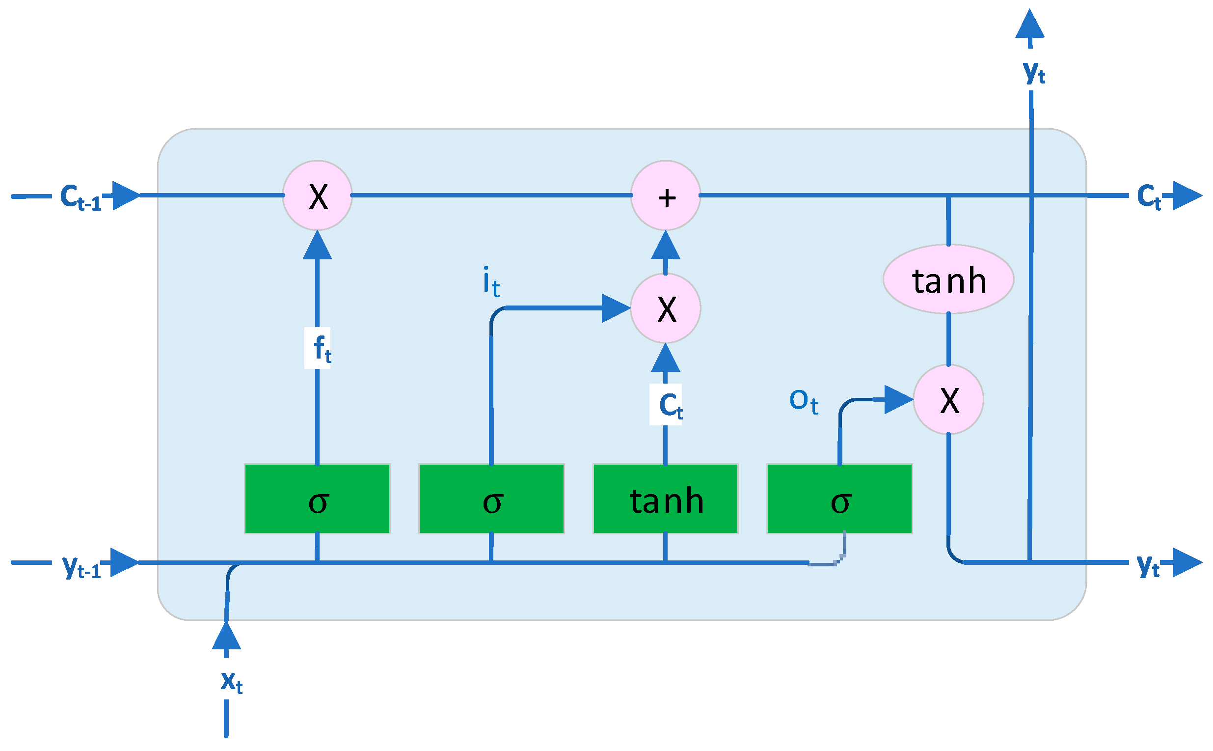
A standard repeating module/recurrent unit with a simple structure (a single tanh layer) is displayed in Figure 1. The diagram of the LSTM recurrent network cell is provided in Figure 2 [41].

The job of the LSTM neural network is to learn how to match an input $x=\left(x_1,\dots ,x_T\right)$ to an output $y=\left(y_1,\dots ,y_T\right)$ over T iterations ($t=1,\dots ,T$). For each cell, the self-loop weight is controlled by the forget gate defined using the sigmoid function

$$f_t=\sigma \left( b_f+U_f·x_t+W_f·y_{t-1}\right),$$

(17)

where $U_f$, $W_f$ and $b_f$ are, respectively, the input weights, the recurrent weights and the bias.

The external input gate is computed similarly to the forget gate value using the parameters $U_i$, $W_i$ and $b_i$ by

$$i_t=\sigma \left(b_i+U_i·x_t+W_i·y_{t-1}\right).$$

(18)

The new candidate values are computed in ${\tilde{c}}_t$ by a tanh layer

$${\tilde{c}}_t=tanh\left(b_c+U_c·x_t+W_c·y_{t-1}\right),$$

(19)

where $U_c$, $W_c$ and $b_c$ are, respectively, the input weights, the recurrent weights and the bias corresponding to the cell gate.

The LSTM cell internal state $c_{t-1}$ is updated with the conditional self-loop weight according to

$$c_t=f_t°c_{t-1}+i_t°{\tilde{c}}_t,$$

(20)

where $°$ denotes the Hadamar product.

The output of the LSTM cell is given by

$$y_t=o_t °tanh\left(c_t\right)$$

(21)

$$o_t=\sigma \left(b_o+U_o·x_t+W_o·y_{t-1}\right),$$

(22)

where $U_o$, $W_o$ and $b_o$ are, respectively, the input weights, the recurrent weights and the bias and $o_t$ is the value of the output gate at the time t.

The number of hidden neurons is different from one application to another and it depends on the specifics of the application: the size of the input and output and the number of training samples. One of the most commonly used ways to define the dimension of the hidden layer is expressed as follows [42]:

$$\left|F_H\right|=2\left[\sqrt{\left(\left|F_Y\right|+2\right)\left|F_X\right|}\right],$$

(23)

where $\left|F_X\right|$ is the size of the input layer and $\left|F_Y\right|$ is the number of neurons in the output layer.

In our work, we used an ADAM optimizer to train LSTMs, since it is one of the most successfully applied algorithms, it is well suited for nonstationary complex objectives and it is computationally efficient [43].

4.3. ES-LSTM Method

The proposed method, ES-LSTM, consists of two stages. We denote by $S=\left(X, Y\right)$ the available training data. In the first stage, a standard LSTM neural network is trained using the first $n\_tr$ samples of each input, denoted by $S^{LSTM}$. The standard LSTM architecture consists in a sequence input, an LSTM layer, a fully connected layer and a regression output layer. Our model uses an ADAM training algorithm and MSE loss function. The LSTM layer of the resulting trained neural network comprises three learnable parameters: the input weights matrix U, the recurrent weights matrix W and the bias vector b. Each parameter is the concatenation of its four correspondents in the gates of the LSTM layer described in Section 4.2, that is, $U=\left[\begin{array}{c}\begin{array}{c}{U}_i\\ U_f\\ U_c\end{array}\\ U_o\end{array}\right]$, $W=\left[\begin{array}{c}\begin{array}{c}{W}_i\\ W_f\\ W_c\end{array}\\ W_o\end{array}\right]$ and $b=\left[\begin{array}{c}\begin{array}{c}{b}_i\\ b_f\\ b_c\end{array}\\ b_o\end{array}\right]$. In the second stage, the 2MES algorithm updates U, W and b to maximize a fitness function measuring the accuracy of the network in terms of trend prediction and MAPE value. In this stage, the whole set of training data is processed.

We denote by $P_0=\left(U_0,W_0,b_0\right)$ the parameter computed by the first stage of the ES-LSTM algorithm and let $F{1}_0$, $MAP{E}_0$ and $RMS{E}_0$ be the values of accuracy indicators (3), (4) and (9) produced by the trained LSTM on $S$. The 2MES local search starts with $P_0$ and computes a sequence $P_1,P_2,\dots ,P_{NMAx}$ using the fitness function defined by

$$fitness\left(P_i\right)=ct·\frac{1}{MAP{E}_i}+F{1}_i,$$

(24)

where ct is a positive constant indicating the balance between the error MAPE and the trend prediction indicator F1 and $F{1}_i$ and $MAP{E}_i$ and $RMS{E}_i$ are the values of quality indicators produced by the LSTM having the learnable parameter $P_i$. Note that, during the evolution, the RMSE value should also be controlled.

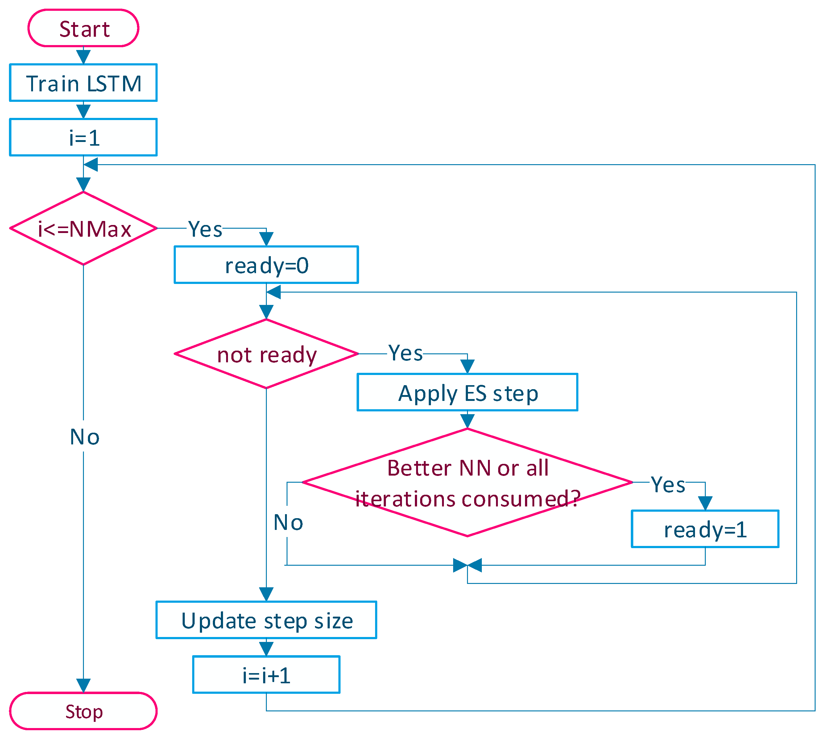
We denote by NMax the maximum number of iterations and by $\sigma , \tau$ and $\vartheta$ the 2MES parameters described in Section 4.1. Note that the 2MES parameter updating rule (16) is adapted to the proposed Algorithm 1, in the sense that it takes into account the number of attempts needed to improve the fitness value in order to modify the value of the parameter $\sigma$. The parameter NAtt is the maximum number of attempts performed at one evolution step in order to improve the fitness value. Let $\epsilon >0$ be a parameter controlling the RMSE. If A is an array, we denote by $N_A\left(0,\sigma \right)$ an array with the same dimensions as A, whose elements are randomly generated from the normal distribution $N\left(0,\sigma \right)$. The resulting algorithm is provided below.

Algorithm 1:

Inputs. $S$, $S^{LSTM}$, ct, NMax, NAtt, $\sigma , \tau$, $\vartheta$ and $\epsilon$

Step 1. Train the LSTM neural network using $S^{LSTM}$ and obtain $P_0=\left(U_0,W_0,b_0\right).$

Step 2. Compute $F{1}_0$, $MAP{E}_0$ and $RMS{E}_0$ using $S$ and (3), (4) and (9).

Step 3. for i =1..NMax

3.1. ok$\leftarrow$0; nr_a$\leftarrow$0;

3.2. while not ok

3.2.1. Compute $P_i=\left(U_i,W_i,b_i\right)$.

$U_i\leftarrow U_{i-1}+N_U\left(0,\sigma \right)$; $W_i\leftarrow W_{i-1}+N_W\left(0,\sigma \right)$; $b_i\leftarrow b_{i-1}+N_b\left(0,\sigma \right)$         3.2.2. nr_a$\leftarrow$ nr_a+1

3.2.3. Compute $F{1}_i$, $MAP{E}_i$ and $RMS{E}_i$ using $S$ and (3), (4) and (9).

3.2.4. if $fitness\left(P_i\right)>fitness\left(P_{i-1}\right)$ and $RMS{E}_i<RMS{E}_{i-1}\left(1+\epsilon \right)$            ok$\leftarrow$1

3.2.5. if nr_a=NAtt

ok$\leftarrow$1; $P_i\leftarrow P_{i-1}$

3.3. if nr_a<$\tau$

$\sigma \leftarrow \raisebox{1ex}{$\sigma $}\!\left/ \!\raisebox{-1ex}{$\vartheta $}\right.$

else if nr_a$>\tau$

$\sigma \leftarrow \sigma ·\vartheta$

Outputs: LSTM corresponding to $P_{NMAx}$.

The flowchart in Figure 3 summarizes the proposed algorithm.

Note that the ES-LSTM algorithm is computationally efficient since it uses only one individual per iteration and only one evolution operator. Bear in mind that the reviewed methods use population-based evolutionary approaches, which are far more expensive from the run time point of view. The reviewed evolutionary methods require and use several operators to accomplish the evolution. In many cases, they use binary representation, which requires supplementary time for encoding and decoding.

5. Experiments

The proposed method was implemented to train LSTMs on three datasets containing the daily exchange rates for three currencies: BTC–USD, ETH–USD and EUR–USD, available in [44]. The data range of each time series is from 18 November 2016 to 15 April 2022. The data do not include weekends and the main international legal days off.

The tests were performed using MATLAB 2019a software, running on a laptop with the following configuration: processor Intel Core i7-10870H up to 5.0 GHz, 16 GB RAM DDR4, SSD 512 GB, and NVIDIA GeForce GTX 1650Ti 4 GB GDDR6.

In order to define the particular NARX forecasting model, the exogenous inputs have to be selected and preprocessed. In our work, we investigated some of the most commonly used technical indicators together with asset-related variables to establish the most promising prediction model. The exogenous inputs taken into account are the filtered versions of the following data: the target, the exponential moving average indicator, the Bollinger frequency bands and the opening, lower and higher prices, respectively [45,46]. The inputs’ selection has been performed by measuring the LSTM performances in terms of RMSE and MAPE in training and testing the NARX model. In case of the EUR/USD time series, 30% of data was used to test the model, while 10% of data was used for prediction of both BTC and ETH recorded sets. The simulations were conducted with delay parameters computed using the correlogram-based analysis performed for each time series. For all analyzed records, the best model in terms of LSTM’s forecasting performance uses a single exogenous input, namely the filtered version of target data. Note that the selection of the input variables conducted by various methods, for instance, cross-correlation-based feature selection, the peeling algorithm and clustered variable selection based on SVMs [47], led to similar results.

Consequently, if we denote by ${\widehat{Y}}_t$ the predicted value of $Y_t$, $1\le t\le N$, the resulting NARX forecasting model is given by

$${\hat{Y}}_{\left(t+1\right)}=f\left(Y_t,Y_{t-1},\dots ,Y_{t-d_Y+1},Y_t,X_{t-1},\dots ,X_{t-d_X+1}\right),$$

(25)

where Y is the target with the delay variable $d_Y$, X is the exogenous input represented by the filtered version of Y and f is a nonlinear function.

The experimentally established results concerning the performances of the proposed method versus the standard LSTM neural network optimizer designed to implement (25) are reported below. Note that in our tests the available data were split into a training set and test set.

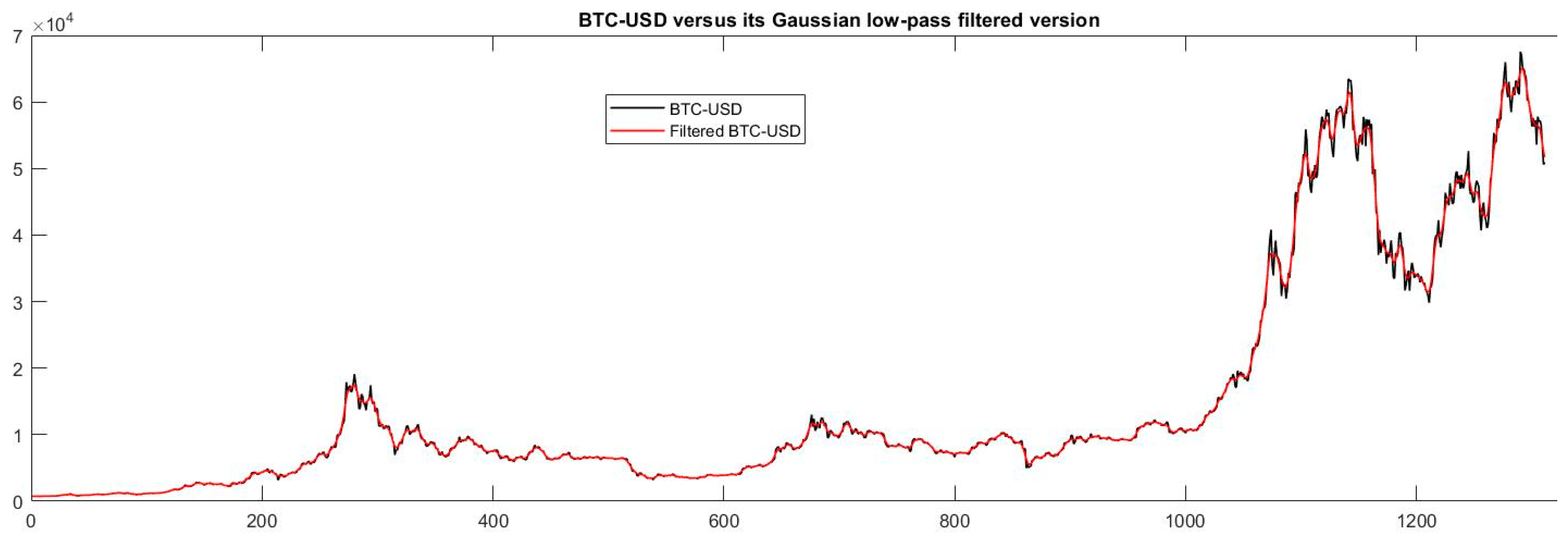
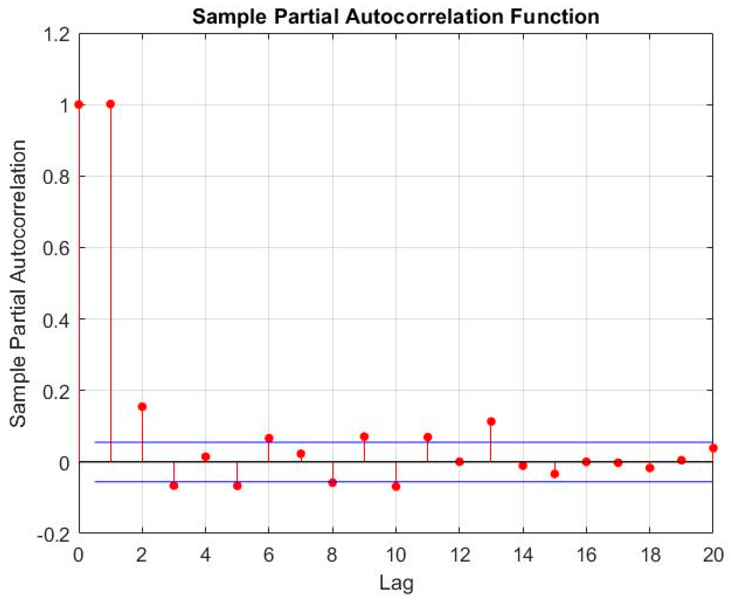
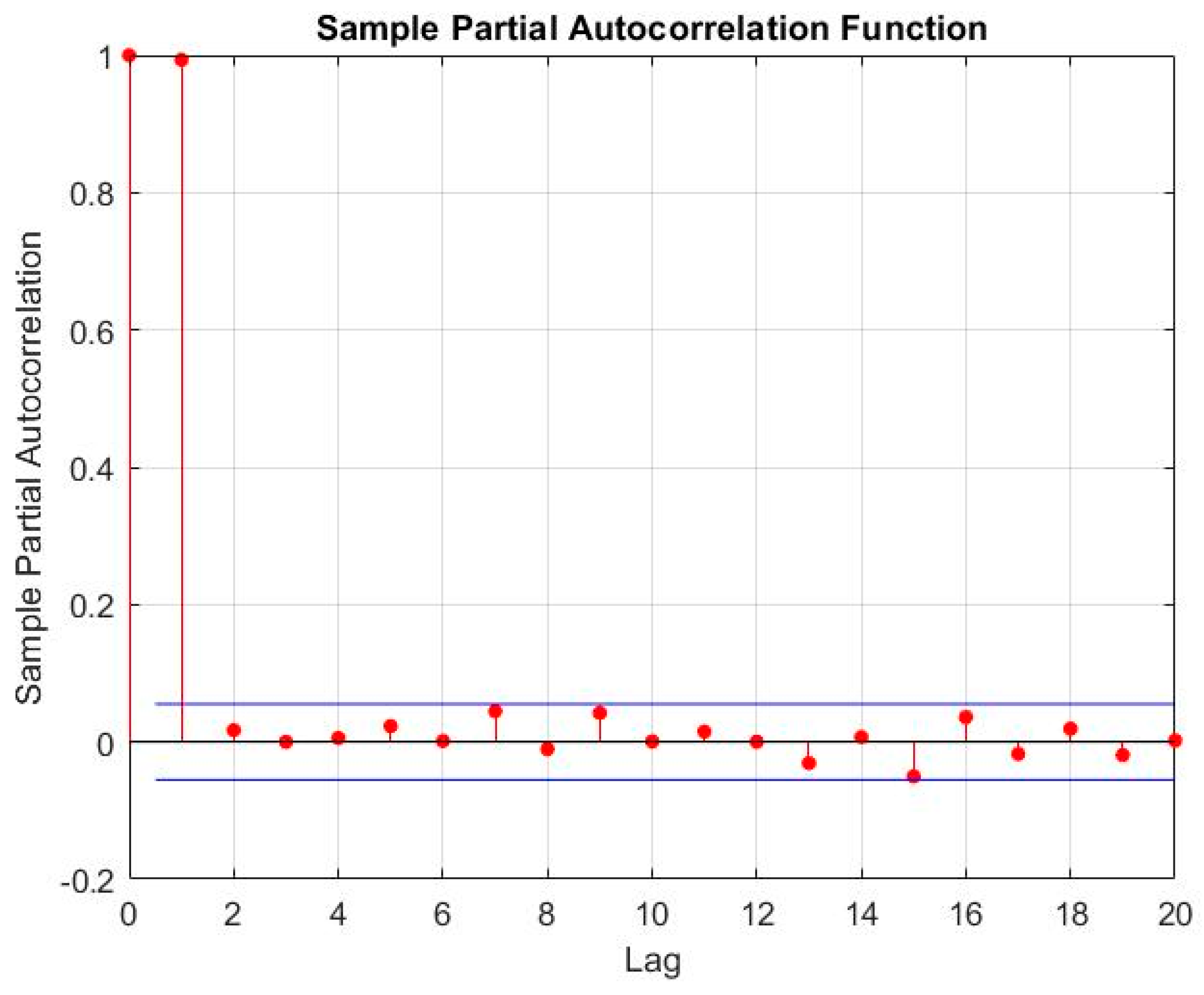
a. The delay variable of the BTC–USD daily exchange rate was computed using partial autocorrelation function (PACF). The result of PACF analysis is provided in Figure 4. The target together with its filtered version representing the selected exogenous input are depicted in Figure 5.

Based on the correlogram analysis, the delay variable was 1. In our tests, we set the delay window to $\left\{1,2, 3, 4\right\}$. Since the second input time series was the low-pass filtered version of the target, we set the same delay window for $d_x$. The best results were obtained for $d_x=d_Y=1$. The dataset was split as follows: standard LSTM: 50 test data and 1260 training data; ES-LSTM: 50 test data and 1260 training data—1195 LSTM and 1260 ES improvement.

Each method was tested 30 times, and the mean values of the trend metrics together with mean RMSE and MAPE errors are provided in

Table 1. BTC–USD: accuracy comparison.

	RMSE	MAPE	F1	POCID
LSTM—training	508.18	2.77	0.690	65.36
ES-LSTM—training	525.27	2.77	0.705	67.58
LSTM—test	3906.25	4.423	0.541	57.77
ES-LSTM—test	3935.64	4.327	0.601	62.99

. The ANOVA analyses of the pairs of MAPE, F1 and POCID values are presented for both training and test data in Figure 6, Figure 7, Figure 8, Figure 9, Figure 10 and Figure 11. Note that the first class corresponds to the LSTM method and the second class corresponds to the proposed ES-LSTM method.

ANOVA test—training data results

1.

MAPE indicator. The result indicates a similarity between the MAPE values.

Figure 6. ANOVA test, MAPE indicator.

Figure 6. ANOVA test, MAPE indicator.

2.

F1 indicator. The result indicates a dissimilarity between the F1 values, the one corresponding to the proposed method being better.

Figure 7. ANOVA test, F1 indicator.

Figure 7. ANOVA test, F1 indicator.

3.

POCID indicator. The result indicates a dissimilarity between the POCID values, the one corresponding to the proposed method being significantly better.

Figure 8. ANOVA test, POCID indicator.

Figure 8. ANOVA test, POCID indicator.

ANOVA test—test data results

1.

MAPE indicator. The result indicates a similarity between the MAPE values.

Figure 9. ANOVA test, MAPE indicator.

Figure 9. ANOVA test, MAPE indicator.

2.

F1 indicator. The result indicates a dissimilarity between the F1 values, the one corresponding to the proposed method being significantly better.

Figure 10. ANOVA test, F1 indicator.

Figure 10. ANOVA test, F1 indicator.

3.

POCID indicator. The result indicates a dissimilarity between the POCID values, the one corresponding to the proposed method being significantly better.

Figure 11. ANOVA test, POCID indicator.

Figure 11. ANOVA test, POCID indicator.

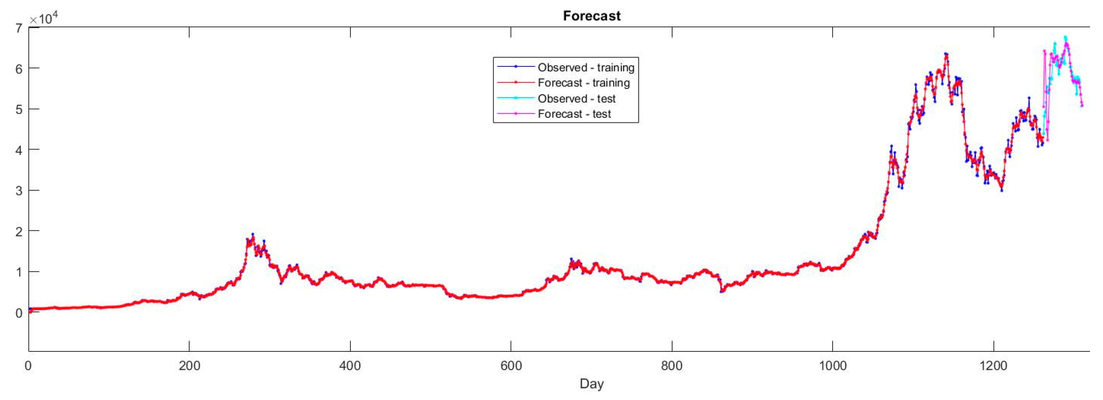
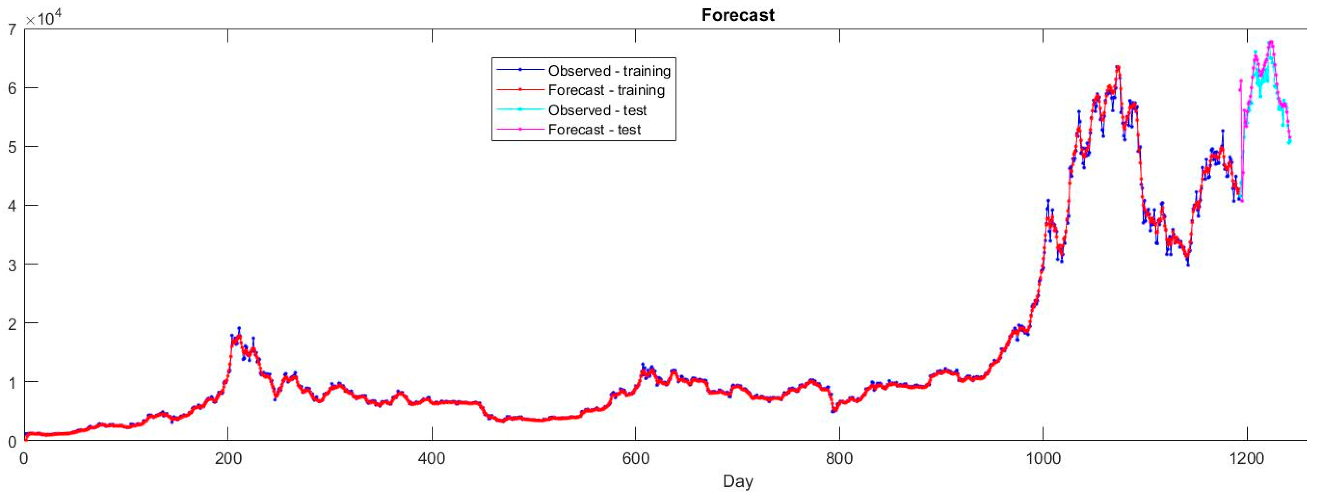
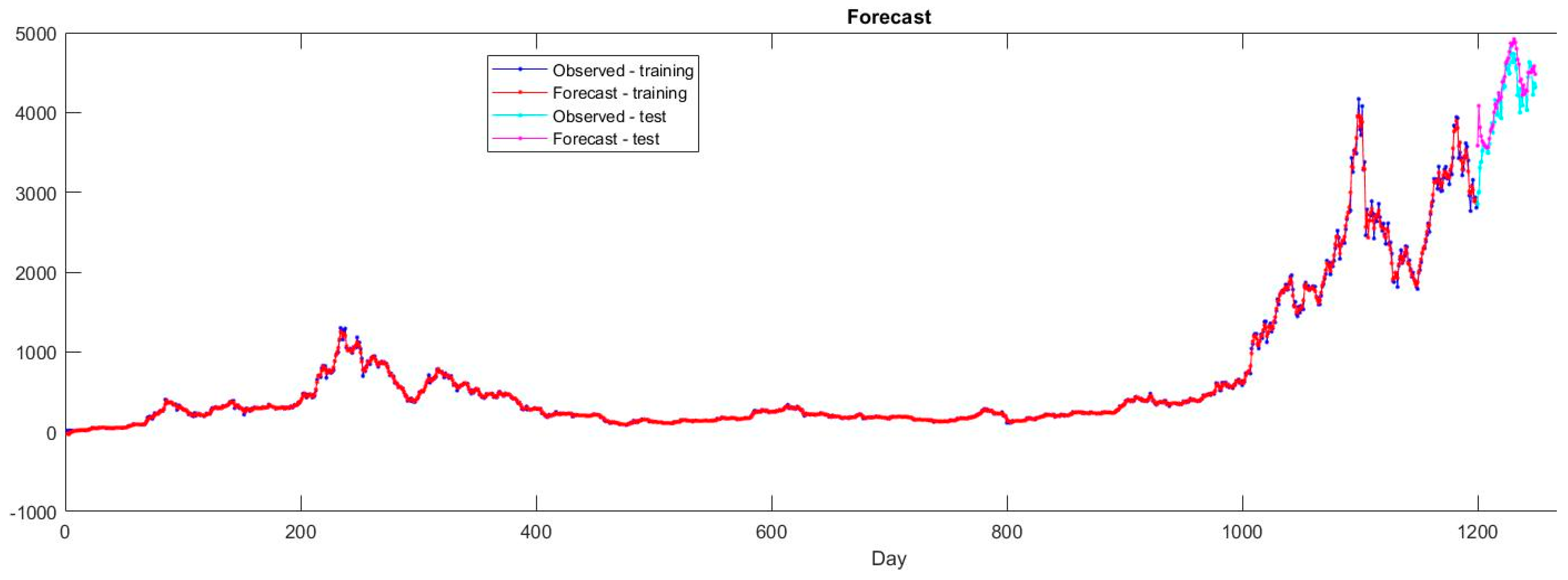
The results of training and testing the LSTM neural network to implement (25) using an ADAM optimizer are depicted in Figure 12. The actual values of BTC–USD time series versus the forecasted outcomes in the case of the proposed ES-LSTM algorithm are presented in Figure 13. The parameters used by the ES-LSTM algorithm were: $ct=0.025$, $NMax=9$, $NAtt=200$, $\sigma =0.01$, $\tau =15$, $\vartheta =0.9$ and $\epsilon =0.1$. The figures present the results of one of the 30 runs.

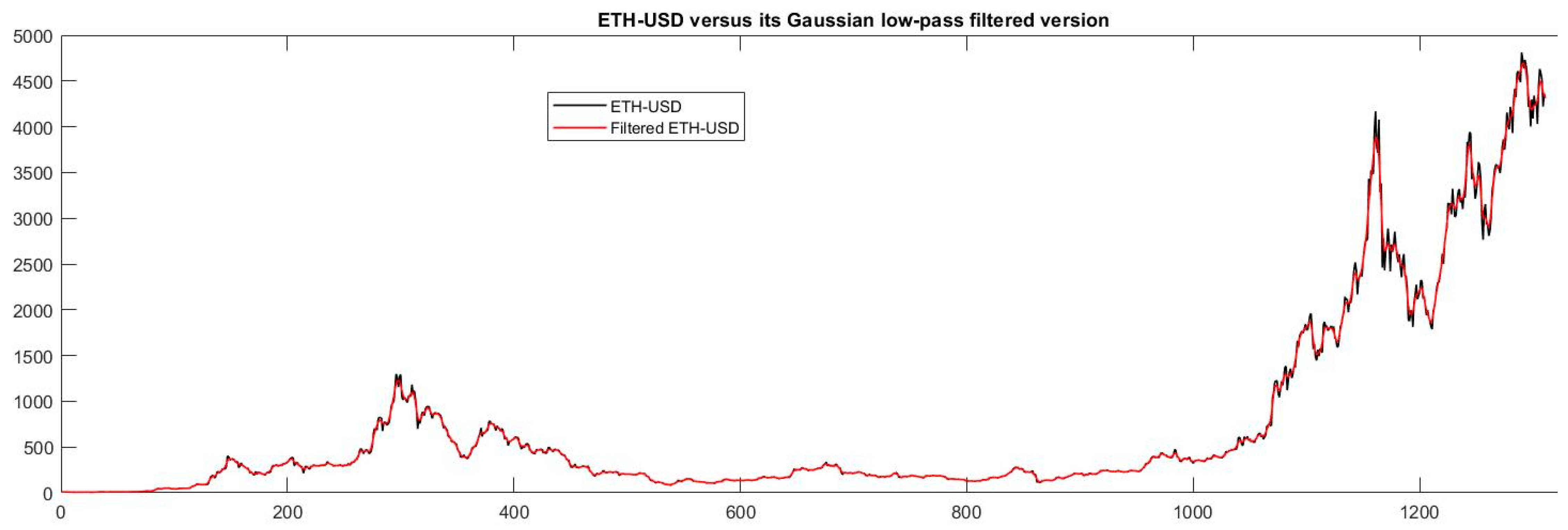
b. The correlogram analysis of the ETH–USD data is provided in Figure 14. The target variable together with its filtered version are presented in Figure 15.

Using the PACF values, the resulting delay parameter was 1. In our tests, we considered the delay window $\left\{1,2, 3, 4\right\}$. The best results were obtained for $d_x=d_Y\in \left\{1,2\right\}$. The results presented below were obtained for $d_x=d_Y=1$.

The dataset was split as follows: standard LSTM: 50 test data and 1260 training data; ES-LSTM: 50 test data and 1260 training data—1195 LSTM and 1260 ES improvement.

Each method was tested 30 times, and the mean values of the trend metrics together with mean RMSE and MAPE errors are provided in

Table 2. ETH–USD: accuracy comparison, delay = 1.

	RMSE	MAPE	F1	POCID
LSTM—training	28.17	6.54	0.693	67.51
ES-LSTM—training	30.23	3.93	0.714	69.84
LSTM—test	315.89	5.73	0.648	61.59
ES-LSTM—test	304.46	5.49	0.673	63.33

. The ANOVA analyses of the pairs of MAPE, F1 and POCID values are presented for both the training and test data in Figure 16, Figure 17, Figure 18, Figure 19, Figure 20 and Figure 21. Note that the first class corresponds to the LSTM method and the second class corresponds to the proposed ES-LSTM method.

ANOVA test—training data results

1.

MAPE indicator. The result indicates a dissimilarity between the MAPE values, the one corresponding to the proposed method being far better.

Figure 16. ANOVA test, MAPE indicator.

Figure 16. ANOVA test, MAPE indicator.

2.

F1 indicator. The result indicates a dissimilarity between the F1 values, the one corresponding to the proposed method being far better.

Figure 17. ANOVA test, F1 indicator.

Figure 17. ANOVA test, F1 indicator.

3.

POCID indicator. The result indicates a dissimilarity between the POCID values, the one corresponding to the proposed method being significantly better.

Figure 18. ANOVA test, POCID indicator.

Figure 18. ANOVA test, POCID indicator.

ANOVA test—test data results

1.

MAPE indicator. The result indicates a similarity between the MAPE values.

Figure 19. ANOVA test, MAPE indicator.

Figure 19. ANOVA test, MAPE indicator.

2.

F1 indicator. The result indicates a dissimilarity between the F1 values, and the one corresponding to the proposed method is slightly better.

Figure 20. ANOVA test, F1 indicator.

Figure 20. ANOVA test, F1 indicator.

3.

POCID indicator. The result indicates a relative similarity between the POCID values, but the one corresponding to the proposed method is slightly better.

Figure 21. ANOVA test, POCID indicator.

Figure 21. ANOVA test, POCID indicator.

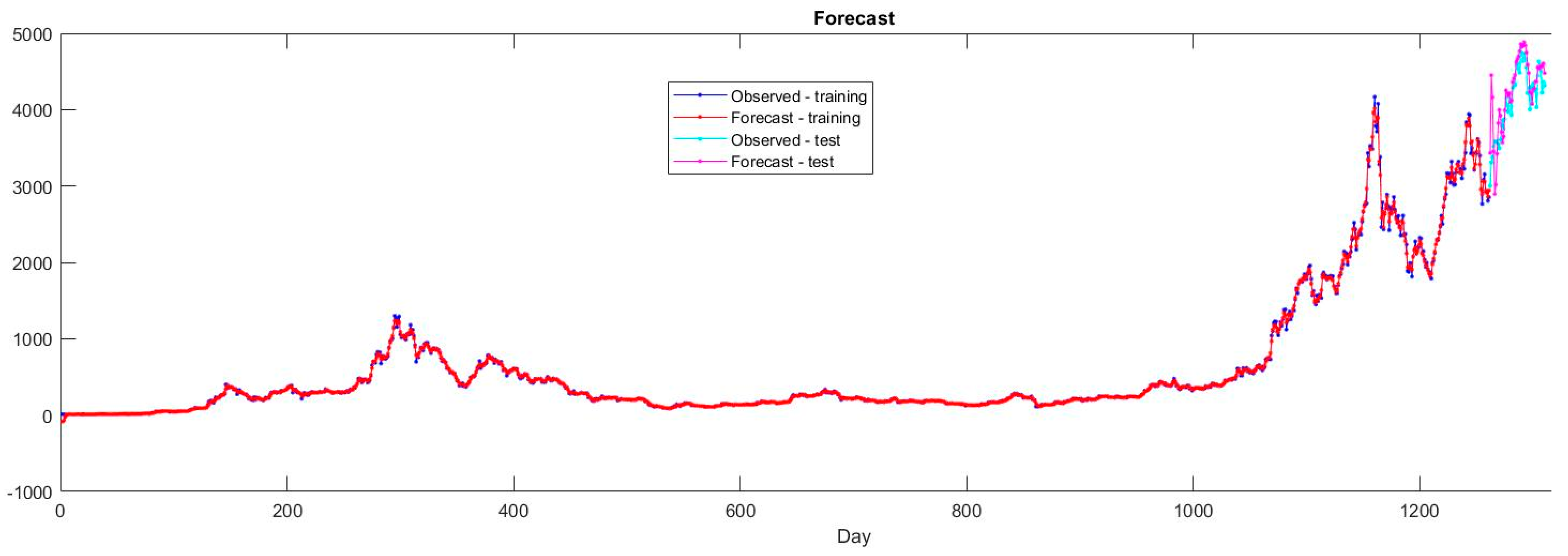
The results of training and testing the LSTM neural network to implement (25) using an ADAM optimizer are depicted in Figure 22. The actual values of ETH–USD time series versus the forecasted outcomes in the case of the proposed ES-LSTM algorithm are presented in Figure 23. The parameters used by the ES-LSTM algorithm were: $ct=0.15$, $NMax=11$, $NAtt=200$, $\sigma =0.01$, $\tau =15$, $\vartheta =0.9$ and $\epsilon =0.01$. The figures present the results of one of the 30 runs.

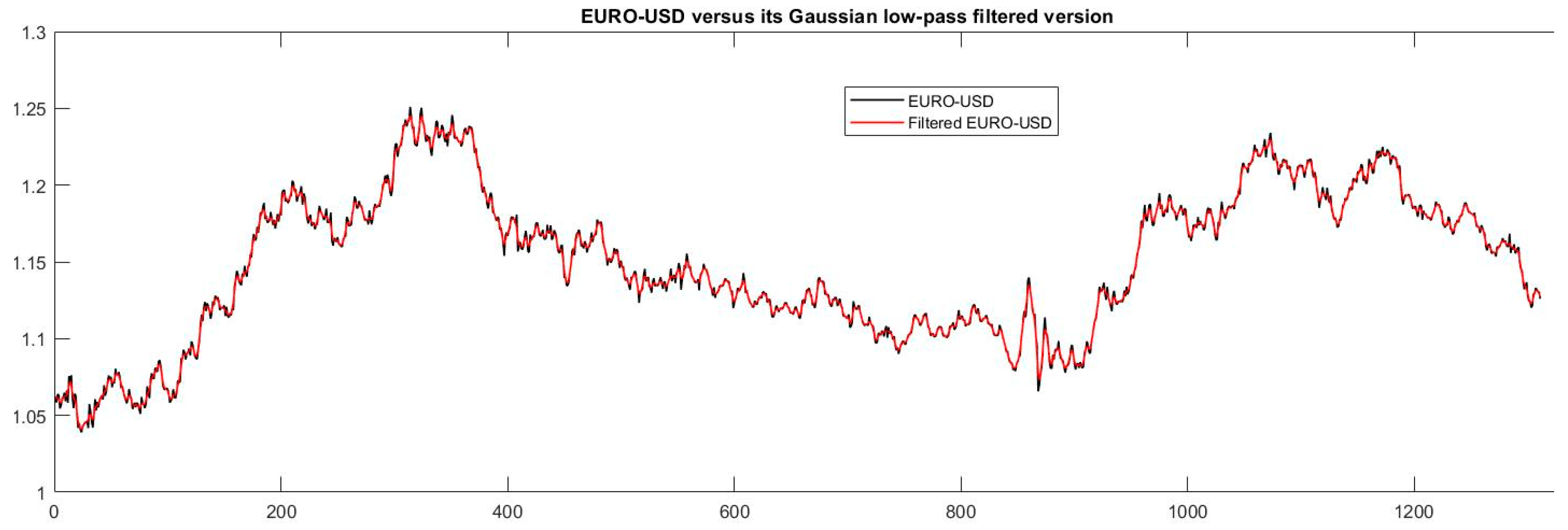
c. The EUR–USD daily exchange rate data analysis is provided below. The PACF analysis (Figure 24) led to the same delay window and the tests indicated that the best results were obtained for delay parameter set to 1. The target time series and the filtered version of it are depicted together in Figure 25.

The dataset was split as follows: standard LSTM: 192 test data (15%) and 1118 training data; ES-LSTM: 192 test data (15%) and 1118 training data—1062 LSTM and 1118 ES improvement.

Each method was tested 30 times, and the mean values of the trend metrics together with mean RMSE and MAPE errors are provided in

Table 3. EUR–USD: accuracy comparison.

	RMSE	MAPE	F1	POCID
LSTM—training	0.0014	0.092	0.888	88.82
ES-LSTM—training	0.0014	0.093	0.901	90.03
LSTM—test	0.0030	0.103	0.836	86.16
ES-LSTM—test	0.0037	0.111	0.856	87.51

. The ANOVA analyses of the pairs of MAPE, F1 and POCID values are presented for both training and test data in Figure 26, Figure 27, Figure 28, Figure 29, Figure 30 and Figure 31. Note that the first class corresponds to the LSTM method and the second class corresponds to the proposed ES-LSTM method. The parameter setting in ES-LSTM was as follows: $ct=0.0005$, $NMax=7$, $NAtt=300$, $\sigma =0.07$, $\tau =15$, $\vartheta =0.9$ and $\epsilon =0.005$.

ANOVA test—training data results

1.

MAPE indicator. The result indicates relatively similar MAPE values.

Figure 26. ANOVA test, MAPE indicator.

Figure 26. ANOVA test, MAPE indicator.

2.

F1 indicator. The result indicates a dissimilarity between the F1 values, the one corresponding to the proposed method being significantly better.

Figure 27. ANOVA test, F1 indicator.

Figure 27. ANOVA test, F1 indicator.

3.

POCID indicator. The result indicates a dissimilarity between the POCID values, the one corresponding to the proposed method being significantly better.

Figure 28. ANOVA test, POCID indicator.

Figure 28. ANOVA test, POCID indicator.

ANOVA test—test data results

1.

MAPE indicator. The result indicates a similarity between the MAPE values.

Figure 29. ANOVA test, MAPE indicator.

Figure 29. ANOVA test, MAPE indicator.

2.

F1 indicator. The result indicates a dissimilarity between the F1 values, the one corresponding to the proposed method being better.

Figure 30. ANOVA test, F1 indicator.

Figure 30. ANOVA test, F1 indicator.

3.

POCID indicator. The result indicates a dissimilarity between the POCID values, the one corresponding to the proposed method being better.

Figure 31. ANOVA test, POCID indicator.

Figure 31. ANOVA test, POCID indicator.

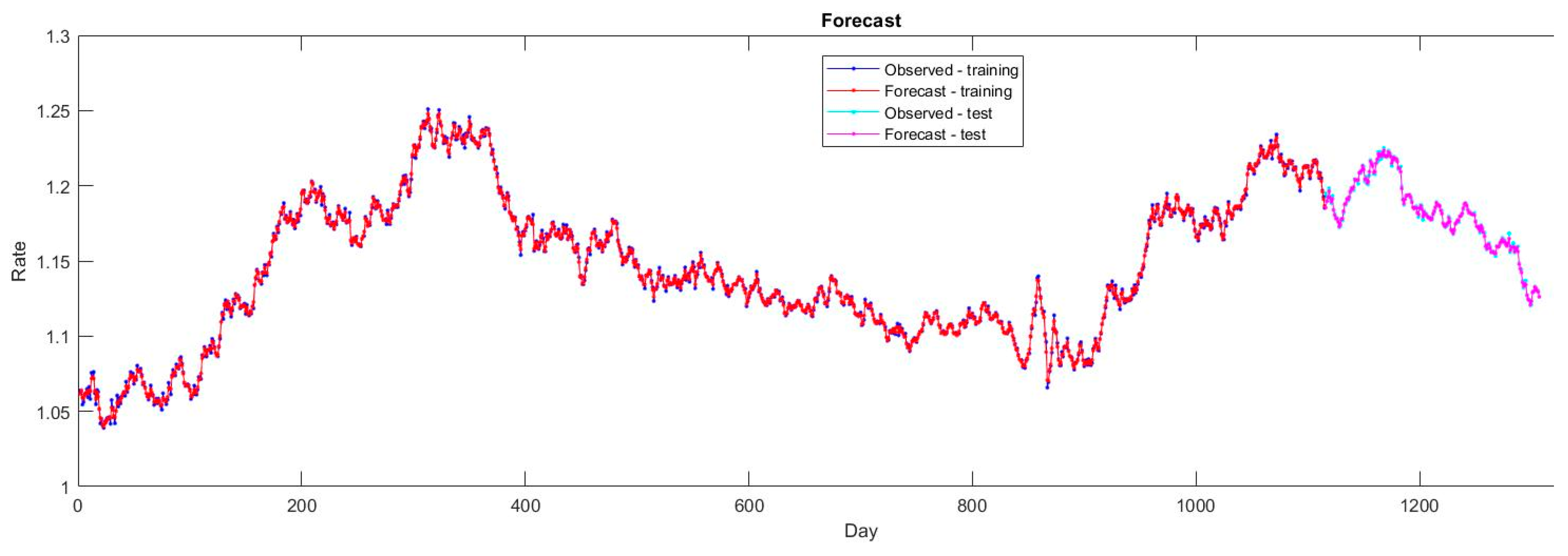
The results of training and testing the LSTM neural network to implement (25) using an ADAM optimizer are depicted in Figure 32. The actual values of EUR–USD time series versus the forecasted outcomes in the case of the proposed ES-LSTM algorithm are presented in Figure 33. The figures present the results of one of the 30 runs.

6. Conclusions and Outlooks

The paper reports a novel evolutionary deep learning technique to analyze and forecast financial time series. The main objective was to improve the F1 score without significantly increasing the error metric. The proposed approach used 2MES local search to fine-tune the learning parameters of LSTMs implementing the NARX model.

The performances of the proposed algorithm were assessed against the standard LSTM predictor using three datasets containing the daily exchange rate for three currencies: BTC–USD, ETH–USD and EUR–USD. The experimental results proved that our training approach is more accurate in terms of both POCID and F1 measures and, in some cases, the MAPE index is also far better. The results are supported from the theoretical point of view, since the main aim of the 2MES procedure is to optimize a mixture objective function defined in terms of F1 and MAPE. The RMSE values are controlled by the admissibility condition implemented by step 3.2.4 of the proposed method. Note that the ES-LSTM algorithm is also computationally efficient since it uses only one individual per iteration and only one evolution operator.

Further developments could take into account more complex evolutionary methods to tune the learnable parameters of LSTMs using similar fitness functions. In addition, we intend to develop the proposed approach to select the appropriate exogenous data and to tune some hyper-parameters, for instance, the number of hidden neurons. In addition, the new ES-based model to optimize the stacked LSTM neural networks’ training stage is still in progress.

References

1. Sangiorgio, M.; Dercole, F. Robustness of LSTM neural networks for multi-step forecasting of chaotic time series. Chaos Solitons Fractals 2020, 139, 110045. [Google Scholar] [CrossRef]
2. Siami-Namini, S.; Tavakoli, N.; Namin, A.S. The Performance of LSTM and BiLSTM in Forecasting Time Series. In Proceedings of the 2019 IEEE International Conference on Big Data (Big Data), Los Angeles, CA, USA, 9–12 December 2019; pp. 3285–3292. [Google Scholar] [CrossRef]
3. Thapa, S.; Zhao, Z.; Li, B.; Lu, L.; Fu, D.; Shi, X.; Tang, B.; Qi, H. Snowmelt-Driven Streamflow Prediction Using Machine Learning Techniques (LSTM, NARX, GPR, and SVR). Water 2020, 12, 1734. [Google Scholar] [CrossRef]
4. Cocianu, C.; Avramescu, M. The Use of LSTM Neural Networks to Implement the NARX Model. A Case Study of EUR-USD Exchange Rates. Inform. Econ. 2020, 24, 5–14. [Google Scholar] [CrossRef]
5. Massaoudi, M.; Chihi, I.; Sidhom, L.; Trabelsi, M.; Refaat, S.S.; Abu-Rub, H.; Oueslati, F.S. An Effective Hybrid NARX-LSTM Model for Point and Interval PV Power Forecasting. IEEE Access 2021, 9, 36571–36588. [Google Scholar] [CrossRef]
6. Moursi, A.S.A.; El-Fishawy, N.; Djahel, S.; Shouman, M.A. Enhancing PM2.5 Prediction Using NARX-Based Combined CNN and LSTM Hybrid Model. Sensors 2022, 22, 4418. [Google Scholar] [CrossRef]
7. Xu, Z.; Zhang, X. Short-term wind power prediction of wind farms based on LSTM+NARX neural network. In Proceedings of the 2021 International Conference on Computer Engineering and Application (ICCEA), Kunming, China, 25–27 June 2021; pp. 137–141. [Google Scholar] [CrossRef]
8. Zhan, Z.-H.; Li, J.-Y.; Zhang, J. Evolutionary deep learning: A survey. Neurocomputing 2022, 483, 42–58. [Google Scholar] [CrossRef]
9. Li, Y.; Zhu, Z.; Kong, D.; Han, H.; Zhao, Y. EA-LSTM: Evolutionary attention-based LSTM for time series prediction. Knowl.-Based Syst. 2019, 181, 104785. [Google Scholar] [CrossRef]
10. Zhou, Y.; Guo, S.; Chang, F.-J. Explore an evolutionary recurrent ANFIS for modelling multi-step-ahead flood forecasts. J. Hydrol. 2019, 570, 343–355. [Google Scholar] [CrossRef]
11. Kim, K.-J.; Han, I. Genetic algorithms approach to feature discretization in artificial neural networks for the prediction of stock price index. Expert Syst. Appl. 2000, 19, 125–132. [Google Scholar] [CrossRef]
12. Amjady, N.; Keynia, F. Short-term load forecasting of power systems by combination of wavelet transform and neuro-evolutionary algorithm. Energy 2009, 34, 46–57. [Google Scholar] [CrossRef]
13. Rout, A.K.; Dash, P.; Dash, R.; Bisoi, R. Forecasting financial time series using a low complexity recurrent neural network and evolutionary learning approach. J. King Saud Univ. Comput. Inf. Sci. 2017, 29, 536–552. [Google Scholar] [CrossRef]
14. Kim, K.-J. Artificial neural networks with evolutionary instance selection for financial forecasting. Expert Syst. Appl. 2006, 30, 519–526. [Google Scholar] [CrossRef]
15. Xia, P.; Ni, Z.; Zhu, X.; He, Q.; Chen, Q. A novel prediction model based on long short-term memory optimised by dynamic evolutionary glowworm swarm optimisation for money laundering risk. Int. J. Bio-Inspired Comput. 2022, 19, 77–86. [Google Scholar] [CrossRef]
16. Kumar, R.; Kumar, P.; Kumar, Y. Two-phase hybridisation using deep learning and evolutionary algorithms for stock market forecasting. Int. J. Grid Util. Comput. 2021, 12, 573–589. [Google Scholar] [CrossRef]
17. Ortego, P.; Diez-Olivan, A.; Del Ser, J.; Veiga, F.; Penalva, M.; Sierra, B. Evolutionary LSTM-FCN networks for pattern classification in industrial processes. Swarm Evol. Comput. 2020, 54, 100650. [Google Scholar] [CrossRef]
18. Wang, H.; Wang, H.; Xu, K. Evolutionary recurrent neural network for image captioning. Neurocomputing 2020, 401, 249–256. [Google Scholar] [CrossRef]
19. Izidio, D.; Neto, P.D.M.; Barbosa, L.; de Oliveira, J.; Marinho, M.; Rissi, G. Evolutionary Hybrid System for Energy Consumption Forecasting for Smart Meters. Energies 2021, 14, 1794. [Google Scholar] [CrossRef]
20. Chung, H.; Shin, K.-S. Genetic Algorithm-Optimized Long Short-Term Memory Network for Stock Market Prediction. Sustainability 2018, 10, 3765. [Google Scholar] [CrossRef] [Green Version]
21. Almalaq, A.; Zhang, J.J. Evolutionary Deep Learning-Based Energy Consumption Prediction for Buildings. IEEE Access 2018, 7, 1520–1531. [Google Scholar] [CrossRef]
22. Divina, F.; Maldonado, J.T.; García-Torres, M.; Martínez-Álvarez, F.; Troncoso, A. Hybridizing Deep Learning and Neuroevolution: Application to the Spanish Short-Term Electric Energy Consumption Forecasting. Appl. Sci. 2020, 10, 5487. [Google Scholar] [CrossRef]
23. Chen, Y.-H.; Chang, F.-J. Evolutionary artificial neural networks for hydrological systems forecasting. J. Hydrol. 2009, 367, 125–137. [Google Scholar] [CrossRef]
24. Viswambaran, R.A.; Chen, G.; Xue, B.; Nekooei, M. Two-Stage Genetic Algorithm for Designing Long Short Term Memory (LSTM) Ensembles. In Proceedings of the 2021 IEEE Congress on Evolutionary Computation (CEC), Kraków, Poland, 28 June–1 July 2021; pp. 942–949. [Google Scholar] [CrossRef]
25. Al-Hajj, R.; Assi, A.; Fouad, M.; Mabrouk, E. A Hybrid LSTM-Based Genetic Programming Approach for Short-Term Prediction of Global Solar Radiation Using Weather Data. Processes 2021, 9, 1187. [Google Scholar] [CrossRef]
26. Tsokov, S.; Lazarova, M.; Aleksieva-Petrova, A. A Hybrid Spatiotemporal Deep Model Based on CNN and LSTM for Air Pollution Prediction. Sustainability 2022, 14, 5104. [Google Scholar] [CrossRef]
27. Wibowo, A.; Pujianto, H.; Saputro, D.R.S. Nonlinear autoregressive exogenous model (NARX) in stock price index’s prediction. In Proceedings of the 2017 2nd International conferences on Information Technology, Information Systems and Electrical Engineering (ICITISEE), Yogyakarta, Indonesia, 1–2 November 2017; pp. 26–29. [Google Scholar] [CrossRef]
28. Boussaada, Z.; Curea, O.; Remaci, A.; Camblong, H.; Mrabet Bellaaj, N. A Nonlinear Autoregressive Exogenous (NARX) Neural Network Model for the Prediction of the Daily Direct Solar Radiation. Energies 2018, 11, 620. [Google Scholar] [CrossRef]
29. Di Nunno, F.; Race, M.; Granata, F. A nonlinear autoregressive exogenous (NARX) model to predict nitrate concentration in rivers. Environ. Sci. Pollut. Res. 2022, 29, 40623–40642. [Google Scholar] [CrossRef]
30. Dhussa, A.K.; Sambi, S.S.; Kumar, S.; Kumar, S.; Kumar, S. Nonlinear Autoregressive Exogenous modeling of a large anaerobic digester producing biogas from cattle waste. Bioresour. Technol. 2014, 170, 342–349. [Google Scholar] [CrossRef]
31. Lo, A.; Mamaysky, H.; Wang, J. Foundations of technical analysis: Computational algorithms, statistical inference, and empirical implementation. J. Financ. 2000, 55, 1705–1770. [Google Scholar] [CrossRef]
32. Hyndman, R. Another Look at Forecast Accuracy Metrics for Intermittent Demand. Foresight Int. J. Appl. Forecast. 2006, 4, 43–46. [Google Scholar]
33. Fallahtafti, A.; Aghaaminiha, M.; Akbarghanadian, S.; Weckman, G.R. Forecasting ATM Cash Demand Before and During the COVID-19 Pandemic Using an Extensive Evaluation of Statistical and Machine Learning Models. SN Comput. Sci. 2022, 3, 164. [Google Scholar] [CrossRef]
34. Bansal, A.; Singhrova, A. Performance Analysis of Supervised Machine Learning Algorithms for Diabetes and Breast Cancer Dataset. In Proceedings of the 2021 International Conference on Artificial Intelligence and Smart Systems (ICAIS), Coimbatore, India, 25–27 March 2021; pp. 137–143. [Google Scholar] [CrossRef]
35. Kulkarni, A.; Chong, D.; Batarseh, F.A. 5—Foundations of data imbalance and solutions for a data democracy. In Data Democracy; Batarseh, F.A., Yang, R., Eds.; Academic Press: Cambridge, MA, USA, 2020; pp. 83–106. ISBN 9780128183663. [Google Scholar]
36. Fabrice, D. Financial Time Series Data Processing for Machine Learning. arXiv 2019, arXiv:1907.03010. [Google Scholar]
37. Barsanti, R.J.; Gilmore, J. Comparing noise removal in the wavelet and Fourier domains. In Proceedings of the 2011 IEEE 43rd Southeastern Symposium on System Theory, Auburn, AL, USA, 14–16 March 2011; pp. 163–167. [Google Scholar] [CrossRef]
38. Eiben, A.; Smith, J. Introduction to Evolutionary Computing; Springer: Berlin, Germany, 2015. [Google Scholar] [CrossRef]
39. Goodfellow, I.; Bengio, Y.; Courville, A. Deep Learning; MIT Press: Cambridge, MA, USA, 2016; ISBN 978-0-262-03561-3. [Google Scholar]
40. Hochreiter, S.; Schmidhuber, J. Long short-term memory. Neural Comput. 1997, 9, 1735–1780. [Google Scholar] [CrossRef] [PubMed]
41. Cocianu, C.; Avramescu, M. New Approaches of NARX-Based Forecasting Model. A Case Study on CHF-RON Exchange Rate. Inform. Econ. 2018, 22, 5–13. [Google Scholar] [CrossRef]
42. Sheela, K.G.; Deepa, S.N. Review on Methods to Fix Number of Hidden Neurons in Neural Networks. Math. Probl. Eng. 2013, 2013, 425740. [Google Scholar] [CrossRef]
43. Diederik, P.; Ba, K.J. Adam: A Method for Stochastic Optimization. In Proceedings of the ICLR (Poster), San Diego, CA, USA, 7–9 May 2015. [Google Scholar]
44. Available online: https://finance.yahoo.com/ (accessed on 1 May 2022).
45. Grebenkov, D.S.; Serror, J. Following a trend with an exponential moving average: Analytical results for a Gaussian model. Phys. A Stat. Mech. Its Appl. 2014, 394, 288–303. [Google Scholar] [CrossRef] [Green Version]
46. Butler, M.; Kazakov, D. A learning adaptive Bollinger band system. In Proceedings of the IEEE Conference on Computational Intelligence on Financial Engineering and Economics, New York, NY, USA, 29–30 March 2012; pp. 1–8. [Google Scholar]
47. Cocianu, C.; Hakob, G. Machine Learning Techniques for Stock Market Prediction. A Case Study Of Omv Petrom. Econ. Comput. Econ. Cybern. Stud. Res. 2016, 50, 63–82. [Google Scholar]
Figure 1. Standard recurrent unit.
Electronics 11 02935 g001
Figure 2. Standard LSTM cell.
Electronics 11 02935 g002
Figure 3. Brief description of the proposed algorithm.
Electronics 11 02935 g003
Figure 4. BTC–USD: PACF analysis.
Electronics 11 02935 g004
Figure 5. BTC–USD data set versus its filtered version.
Electronics 11 02935 g005
Figure 12. BTC–USD: LSTM–ADAM optimizer training.
Electronics 11 02935 g012
Figure 13. BTC–USD: ES-LSTM training.
Electronics 11 02935 g013
Figure 14. ETH–USD: PACF analysis.
Electronics 11 02935 g014
Figure 15. ETH–USD data set versus its filtered version.
Electronics 11 02935 g015
Figure 22. ETH–USD: LSTM–ADAM optimizer training.
Electronics 11 02935 g022
Figure 23. ETH–USD: ES-LSTM training.
Electronics 11 02935 g023
Figure 24. EUR–USD: PACF analysis.
Electronics 11 02935 g024
Figure 25. EUR–USD data set versus its filtered version.
Electronics 11 02935 g025
Figure 32. EUR–USD: LSTM–ADAM optimizer training.
Electronics 11 02935 g032
Figure 33. EUR–USD: ES-LSTM training.
Electronics 11 02935 g033