Positioning Algorithm of MEMS Pipeline Inertial Locator Based on Dead Reckoning and Information Multiplexing

Abstract

High-precision mapping and positioning of urban underground pipelines are the basic requirements of urban digital construction. Aiming at the above problems, a dead reckoning algorithm based on the starting point and ending point correction and forward and reverse solution information reuse is proposed. This paper firstly establishes a dead reckoning system model consisting of a microelectromechanical system (MEMS) inertial measurement unit (IMU) and an odometer and analyzes the propagation mechanism of dead reckoning errors. The algorithm constructs the trajectory correction matrix by using the position information of the starting point and the ending point of the short-distance underground pipeline and then uses the trajectory correction matrix to correct the trajectory position information obtained by forward and reverse dead reckoning. Finally, the corrected forward and reverse trajectory position information is fused and averaged to achieve high-precision mapping and positioning of underground pipelines. The simulation results of the 100 m pipeline show that the maximum positioning error of the proposed algorithm for straight pipelines is within 5 cm, and the maximum positioning error for 90° curved pipelines is within 20 cm. The algorithm effectively solves the problem of a rapid accumulation of errors over time in the process of dead reckoning, which greatly improves the positioning accuracy.

1. Introduction

Urban underground pipelines are the infrastructure of urban planning. The pipeline network buried deep in the city is widely used in water supply and drainage, oil and gas transportation, communication cable transmission, and other fields. It is also an important infrastructure for urban planning and management. The precise positioning and mapping of underground pipelines are an important part of smart city construction. At present, the detection and positioning methods of underground pipelines mainly include: electromagnetic wave method (geological radar method), seismic wave method, high-precision magnetic measurement method, high-density electrical method, etc. [1,2,3,4,5]. Although the above methods have their own advantages, it is difficult to realize the inspection of deeply buried nonmetallic pipelines, and the detection accuracy is relatively low.

In recent years, the positioning method of underground pipelines based on inertial measurement technology has been widely used in the measurement of urban, trenchless, underground, small-diameter pipelines [6,7,8,9,10]. Reduct, a Belgian company, has long been aware of the difficulty in the entry of nonmetallic underground small-bore pipeline personnel and is committed to developing a small-bore pipeline measurement system based on inertial technology. WMF Al-Masri et al. proposed a high-precision inertial navigation system for the pipeline inspection instrument, which was verified by experiments combined with the corresponding algorithm [11]. In the aspect of a pipeline positioning algorithm based on inertial technology, Niu Xiaoji et al. analyzed the feasibility of the integrated navigation algorithm scheme based on an MEMS inertial device odometer, combined with motion constraints and reverse smoothing for small-diameter pipeline positioning and used the STIM300 gyroscope to verify the effectiveness of the proposed algorithm [12,13]. On the basis of analyzing the error propagation characteristics of inertial navigation, Huang Feirong et al. proposed an inverse solution scheme based on marker points to improve the accuracy of comprehensive navigation and positioning [14]. Sahli Hussein proposed an algorithm based on a low-cost inertial measurement unit using an extended Kalman filter and pipeline node information fusion, which solved the problem of low positioning accuracy when ground markers were unavailable, and achieved beneficial effects [15]. The above three algorithms all use the known information of external markers or pipeline nodes and the microinertial navigation system (MINS) to form an integrated navigation system and use the Kalman filter method for error estimation and correction to achieve high pipeline positioning accuracy [16,17,18]. The positioning method of this integrated navigation is greatly affected by the accuracy of the model construction, and there are problems, such as the decrease in the positioning accuracy of the integrated navigation system when the external measurement information is inaccurate. Liu Jianwei et al. developed a pipeline measuring instrument composed of data acquisition and data processing parts, using complementary filtering and dead reckoning methods combined with offline data trajectory correction, and obtained beneficial measurement results. The horizontal positioning error of the 100 m straight pipeline experiment is 0.13 m [19]. However, the modified method only uses the end point information; the information utilization rate is low; the positioning effect of short and straight pipelines is obvious, and the positioning accuracy of curved pipelines is low.

Aiming at the problem of high-precision mapping and positioning of urban, underground, short-distance, trenchless small-diameter pipelines, this paper proposes a dead reckoning algorithm based on the start and end point correction and forward and reverse solution information multiplexing. The 10°/h gyroscope was used for simulation experiments. The simulation results of 100 m pipeline length show that the maximum positioning error of the algorithm for straight pipelines was within 5 cm, and the maximum positioning error for 90° curved pipes was within 20 cm. The algorithm proposed in this paper effectively solves the problem of the rapid accumulation of the error of the line position estimation over time, and the positioning accuracy is improved by about two times, which has important practical engineering value.

2. Mathematical Model of Dead Reckoning for Pipeline Inertial Locator

2.1. Initial Alignment Model

Because the pipeline inertial locator adopts the dead reckoning algorithm based on inertial technology, it needs to complete the binding and acquisition of initial information, including initial position, initial speed, and initial attitude information, before it enters the working state. When the pipeline inertial locator is working, it starts from one end of the pipeline and travels at a certain speed to the other end. The initial position information is generally consistent with the position information of the starting point of the pipeline. Since the system starts to work from a standstill, the initial speed information is generally set to zero [20].

The accuracy of acquiring initial attitude information (pitch, roll, and heading) directly affects the accuracy of dead reckoning. The measurement accuracy of the pipeline inertial locator is low, and it is difficult to be sensitive to the information of the angular velocity of the Earth’s rotation. Because it uses the MEMS gyroscope device, it cannot use the natural local gravitational acceleration vector and the angular velocity vector of the Earth’s rotation to achieve the initial attitude determination by the method of double vector attitude determination. The MEMS accelerometer can be sensitive to the local gravitational acceleration, and the initial horizontal attitude information can be obtained by measuring the output value of the accelerometer. After the system starts to work, the inertial locator is stationary for 2 min, and the sampled acceleration data are averaged [21]:

$${\overline{\mathit{f}}}_{ib}=\frac{1}{N}{\displaystyle \sum _{k=1}^N{\mathit{f}}_{ib}(k)},N=t/T$$

(1)

where $t$ is the total sampling time; $T$ is the sampling time interval; $N$ is the amount of output data for the MEMS accelerometer in the total sampling time; ${\mathit{f}}_{ib}(k)$ is the acceleration output value of each time interval, and ${\overline{\mathit{f}}}_{ib}$ is the three-dimensional acceleration average value.

The initial pitch angle formula is expressed as:

$$\theta ={\sin }^{-1}\left(\frac{{\overline{f}}_{iby}}{\left|{\overline{\mathit{f}}}_{ib}\right|}\right)$$

(2)

The initial roll angle formula is expressed as:

$$\gamma ={\tan }^{-1}\left(-\frac{{\overline{f}}_{ibx}}{{\overline{f}}_{ibz}}\right)$$

(3)

The initial heading angle is generally given according to the actual direction of the pipeline, namely:

$$\psi ={\sin }^{-1}(\frac{\cos ({\varphi }_1)\sin ({\lambda }_1-{\lambda }_0)}{\sqrt{(1-{\left[\sin {\phi }_0\sin {\phi }_1+\cos {\phi }_0\cos {\phi }_1\cos ({\lambda }_1-{\lambda }_0)\right]}^2}}$$

(4)

where $({\phi }_0,{\lambda }_0)$ is the coordinate of the start point of the pipeline, and $({\phi }_1,{\lambda }_1)$ is the coordinate of the end point of the pipeline.

2.2. Dead Reckoning Model

After the initial alignment is completed, the system enters dead reckoning mode, and the pipeline inertial locator travels along the underground pipeline. Since the system generally runs at a speed of 1 m/s, and the internal sampling time of the system can be set to 0.01 s, the movement distance of the system changes very little during the sampling time interval, so it can be considered that the system moves in a straight line during the sampling time interval. Therefore, the precise position information of the next moment can be determined according to the heading, speed information, and position information of the locator at the previous moment [22]. The principle diagram of dead reckoning is shown in Figure 1.

We selected the east–north–sky coordinate system as the navigation reference coordinate system and recorded it as $n$. The Micro Inertial Measurement Unit (MIMU) was installed in the pipeline inertial locator in the right-front-up manner. It is considered that the MIMU coordinate system coincides with the body coordinate system and is recorded as $b$. At the wheel of the locator, we defined the coordinate system of the odometer and recorded it as $m$. The installation method and its schematic diagram are shown in Figure 2.

The output of the MEMS gyroscope is the angular rate information ${\omega }_{ib}^b$ at time $k$ under the body coordinate system, and the angular increment expression from time $k-1$ to time $k$ is:

$$\Delta \theta ={\displaystyle {\int }_{k-1}^k{\omega }_{ib}^b}dt$$

(5)

The attitude matrix update formula is:

$$C_{b_k}^n=C_{n_{k-1}}^n{C}_{b_{k-1}}^{n_{k-1}}{C}_{b_k}^{b_{k-1}}$$

(6)

where $C_{b_{k-1}}^{n_{k-1}}$ and $C_{b_k}^n$ are the attitude matrices of time $k-1$ and time $k$; the attitude matrix $C_{b_k}^{b_{k-1}}$ represents the body coordinate system transformation caused by the angular motion of the carrier, and the attitude matrix $C_{n_{k-1}}^n$ represents the navigation coordinate system caused by the linear motion of the carrier.

The output of the odometer is the increment information from time $k-1$ to time $k$, and its projection form is:

$$\Delta {\mathit{S}}_k^m={\left[\begin{array}{ccc}0& \Delta S_k& 0\end{array}\right]}^{\mathrm{T}}$$

(7)

Assuming that the installation deviation angle $\mathit{\alpha }$ of the odometer is known and the scale factor error $\delta k=0$, the output expression of the odometer under the navigation coordinate system is:

$$\Delta {\mathit{S}}_k^n={\mathit{C}}_{b_{k-1}}^n(I-\mathit{\alpha }\times )\Delta {\mathit{S}}_k^m$$

(8)

The iterative recursive formula for dead reckoning is:

$$\left\{\begin{array}{l}{\phi }_k={\phi }_{k-1}+\frac{\Delta S_{k(N)}^n}{R_M+h_{k-1}}\\ {\lambda }_k={\lambda }_{k-1}+\frac{\Delta S_{k(E)}^n}{R_N+h_{k-1}}\\ h_k=h_{k-1}+\Delta S_{k(U)}^n\end{array}\right.$$

(9)

where ${\phi }_{k-1}$, ${\lambda }_{k-1}$, and $h_{k-1}$ are the latitude, longitude, and altitude information, respectively, at time $k-1$; $\Delta S_{k(N)}^n$, $\Delta S_{k(E)}^n$, and $\Delta S_{k(U)}^n$ are the mileage information under the navigation coordinate system at time $k$, and $R_M$ and $R_N$ are the radius of curvature of the Earth’s meridional surface and the radius of curvature of the earth’s unitary surface.

3. Dead Reckoning Error Analysis

The main error sources of dead reckoning of the pipeline inertial locator are random gyro drift of the MEME gyroscope, odometer installation deviation angle error, odometer scale factor error, and initial alignment error [23,24].

The gyro drift of MEMS gyroscope is generally divided into two parts: one part is the fixed constant drift, and the other part is the random drift. The fixed constant value drift is usually calibrated in advance through the calibration experiment before the MEMS gyroscope leaves the factory or works to achieve compensation. The random drift cannot be identified in advance due to the difference between each power-on and start-up and then propagates along the error propagation link and affects the dead reckoning positioning accuracy.

The random drift $\mathit{\epsilon }$ of the gyroscope will cause a platform misalignment angle $\mathit{\varphi }$ between the navigation coordinate system and the calculated navigation coordinate system, and its specific expression is:

$$\begin{gathered} \dot{\mathit{\varphi }}=-{\mathit{\omega }}_{in}^n\times \mathit{\varphi }+{\mathit{M}}_{av}\delta {\mathit{v}}^n+{\mathit{M}}_{ap}\delta \mathit{p}-{\mathit{C}}_b^n{\mathit{\epsilon }}^b \\ {\mathit{M}}_{av}=\left[\begin{array}{ccc}0& -\frac{1}{R_M+h}& 0\\ \frac{1}{R_N+h}& 0& 0\\ \frac{\tan \phi }{R_N+h}& 0& 0\end{array}\right] \\ {\mathit{M}}_{ap}=\left[\begin{array}{ccc}0& 0& \frac{v_N}{{(R_M+h)}^2}\\ -{\omega }_{ie}\sin \phi & 0& -\frac{v_E}{{(R_N+h)}^2}\\ {\omega }_{ie}\cos \phi +\frac{v_E{\sec }^2\phi }{R_N+h}& 0& \frac{v_E\tan \phi }{{(R_N+h)}^2}\end{array}\right] \end{gathered}$$

(10)

where ${\mathit{\omega }}_{in}^n$ is the angular velocity caused by the motion of the navigation coordinate system; $\delta {\mathit{v}}^n$ is the velocity error under the navigation coordinate system; $\delta \mathit{p}$ is the position error under the navigation coordinate system; ${\mathit{M}}_{av}$ is the transformation matrix of velocity to platform misalignment angle, and ${\mathit{M}}_{ap}$ is the transformation matrix of position to platform misalignment angle.

The formula for calculating the navigation coordinate system is:

$$C_b^{n\prime }=(I+\mathit{\varphi })C_b^n$$

(11)

Substitute formula (11) into formula (8) without considering the installation deviation angle error $\delta \mathit{\alpha }$ and the odometer scale factor error $\delta k$; then, the actual output expression of the odometer is:

$$\Delta {\tilde{\mathit{S}}}_k^n=(I+{\mathit{\varphi }}_{k-1})C_{b_{k-1}}^n(I-\alpha \times )\Delta {\mathit{S}}_k^m$$

(12)

where $\Delta {\tilde{\mathit{S}}}_k^n$ is the actual output mileage increment of the odometer under the navigation coordinate system; ${\mathit{\varphi }}_{k-1}$ is the platform misalignment angle; $C_{b_{k-1}}^n$ is the ideal attitude transformation matrix, and $\Delta {\mathit{S}}_k^m$ is the mileage increment under the odometer coordinate system.

The dead reckoning error caused by the random drift of the MEMS gyroscope is expressed as:

$$\delta \Delta {\mathit{S}}_k^n=\Delta {\tilde{\mathit{S}}}_k^n-\Delta {\mathit{S}}_k^n={\mathit{\varphi }}_{k-1}{C}_{b_{k-1}}^n(I-\alpha \times )\Delta {\mathit{S}}_k^m$$

(13)

The installation position of the odometer and MIMU in the pipeline inertial locator is shown in Figure 3. During the assembly process, there is always an installation deviation angle between the odometer and the MIMU. The installation deviation angle and scale factor are generally compensated by calibration experiments.

During the calibration process of the odometer, there will always be a calibration residual installation deviation angle error $\delta \alpha$ and a scale factor error $\delta k$. These two errors will gradually accumulate the dead reckoning error with the increase in the mileage of the inertial locator during the dead reckoning process.

The calibration residual installation deviation angle error $\delta \alpha$ is composed of the pitch residual installation deviation angle $\delta {\alpha }_{\theta }$, the roll residual installation deviation angle $\delta {\alpha }_{\gamma }$, and the azimuth residual installation deviation angle $\delta {\alpha }_{\psi }$ that is $\delta \alpha ={\left[\begin{array}{ccc}\delta {\alpha }_{\theta }& \delta {\alpha }_{\gamma }& \delta {\alpha }_{\psi }\end{array}\right]}^{\mathrm{T}}$; the residual installation deviation angle correction matrix ${\mathit{C}}_m^b$ composed of the calibration residual installation deviation angle is:

$${\mathit{C}}_m^b=\left(\mathit{I}+\delta \mathit{\alpha }\times \right)=\left[\begin{array}{ccc}1& -\delta {\alpha }_{\psi }& \delta {\alpha }_{\gamma }\\ \delta {\alpha }_{\psi }& 1& -\delta {\alpha }_{\theta }\\ -\delta {\alpha }_{\gamma }& \delta {\alpha }_{\theta }& 1\end{array}\right]$$

(14)

Considering the odometer scale factor error $\delta k$, the odometer measurement output expression is:

$$\Delta {\tilde{S}}_{}^m=(1+\delta k)\Delta S_{}^m$$

(15)

The actual output expression of the odometer after considering the residual installation deviation angle and the odometer scale factor error is:

$$\Delta {\tilde{S}}_{}^m=(\mathit{I}-\mathit{\alpha }\times )(1+\delta k)\Delta S_{}^m$$

(16)

In summary, the dead reckoning error caused by the random drift $\epsilon$ of the MEMS gyroscope, the installation deviation angle error $\delta \alpha$ of the odometer, and the scale factor error $\delta k$ of the odometer are as follows:

$$\delta \Delta {\mathit{S}}_k^n={\mathit{\varphi }}_{k-1}{C}_{b_{k-1}}^n{\mathit{C}}_{m_k}^b(\mathit{I}-\mathit{\alpha }\times )(1+\delta k)\Delta S_k^m$$

(17)

4. Trajectory Position Error Correction Algorithm

The gyro drift of the MEMS gyroscope in the pipeline inertial locator, the calibration residual installation deviation angle of the odometer, and the scale factor error will make the dead reckoning trajectory different from the real trajectory, making the underground pipeline running trajectory deviation larger, and it is difficult to meet the requirements of centimeter-level mapping and positioning.

Figure 4 is a schematic diagram of the operation of the pipeline inertial locator in the underground trenchless pipeline in actual work.

Aiming at the problem of large trajectory error in dead reckoning, this section proposes a dead reckoning correction algorithm based on the analysis of the above error sources. The dead reckoning trajectory is corrected by constructing a correction matrix using known location information, such as the starting point and ending point of the pipeline, and then the corrected forward and reverse trajectory information is fused and averaged to achieve high-precision mapping and positioning of underground pipelines. A schematic diagram of the algorithm is shown in Figure 5.

4.1. Forward Horizontal and Height Correction Algorithm

As shown in Figure 4, under the traction of hoist 2, the pipeline inertial locator travels from the start point to the end point, where the position information of the start point and the end point can be obtained by other positioning measurement methods, such as the global navigation satellite system (GNSS). In the Cartesian coordinate system, the start point coordinate is defined as $\left(x_{start},y_{start},z_{start}\right)$; the end point coordinate is $\left(x_{end},y_{end},z_{end}\right)$, and the dead reckoning end point coordinate is $\left(x_{end}^c,y_{end}^c,z_{end}^c\right)$.

According to the coordinates of the start point and end point, the true heading angle can be obtained as:

$${\psi }_1^{+}=\frac{180}{\pi }ta{n}^{-1}\left(\frac{x_{end}-x_{start}}{y_{end}-y_{start}}\right)$$

(18)

The true height rotation angle is:

$${\psi }_2^{+}=\frac{180}{\pi }ta{n}^{-1}\left(\frac{x_{end}-x_{start}}{z_{end}-z_{start}}\right)$$

(19)

The heading angle obtained from dead reckoning is:

$${\psi }_3^{+}=\frac{180}{\pi }ta{n}^{-1}\left(\frac{x_{end}^c-x_{start}}{y_{end}^c-y_{start}}\right)$$

(20)

The height rotation angle obtained by dead reckoning is:

$${\psi }_4^{+}=\frac{180}{\pi }ta{n}^{-1}\left(\frac{x_{end}^c-x_{start}}{z_{end}^c-z_{start}}\right)$$

(21)

The horizontal and height scale transformation factors obtained from the real start and end point information and dead reckoning end point information are:

$$K_1^{+}=\frac{\sqrt{(x_{end}-x_{start}\left)\right(y_{end}-y_{start})}}{\sqrt{(x_{end}^c-x_{start}\left)\right(y_{end}^c-x_{start})}}$$

(22)

$$K_2^{+}=\frac{\sqrt{(x_{end}-x_{start}\left)\right(z_{end}-z_{start})}}{\sqrt{(x_{end}^c-x_{start}\left)\right(z_{end}^c-z_{start})}}$$

(23)

where $K_1^{+}$ is the horizontal scaling factor, and $K_2^{+}$ is the height scaling factor.

The forward correction matrix $C_{p+}^n$ is constructed from formulas (18)–(23) as:

$$C_{p+}^n=\left[\begin{array}{ccc}{K}_1^{+}{K}_2^{+}\cos ({\psi }_1^{+}-{\psi }_3^{+})\cos ({\psi }_2^{+}-{\psi }_4^{+})& K_1^{+}{K}_2^{+}\sin ({\psi }_1^{+}-{\psi }_3^{+})& K_1^{+}{K}_2^{+}\cos ({\psi }_1^{+}-{\psi }_3^{+})\sin ({\psi }_2^{+}-{\psi }_4^{+})\\ -K_1^{+}{K}_2^{+}\sin ({\psi }_1^{+}-{\psi }_3^{+})\cos ({\psi }_2^{+}-{\psi }_4^{+})& K_1^{+}{K}_2^{+}\cos ({\psi }_1^{+}-{\psi }_4^{+})& -K_1^{+}{K}_2^{+}\sin ({\psi }_1^{+}-{\psi }_3^{+})\sin {\psi }_1^{+}-{\psi }_4^{+})\\ -K_1^{+}{K}_2^{+}\sin ({\psi }_2^{+}-{\psi }_4^{+})& 0& K_1^{+}{K}_2^{+}\cos ({\psi }_2^{+}-{\psi }_4^{+})\end{array}\right]$$

(24)

The dead reckoning formula based on forward horizontal and height correction is:

$$\Delta {\tilde{\mathit{S}}}_{+}^n={\mathit{C}}_{p+}^n{\mathit{C}}_b^p{\mathit{C}}_m^b(\mathit{I}-\mathit{\alpha }\times )(1+\delta k)\Delta {\mathit{S}}_{}^m$$

(25)

where ${\mathit{C}}_b^p$ is the calculated attitude transformation matrix.

4.2. Inverse Horizontal and Height Correction Algorithm

As shown in Figure 4, under the traction of hoist 1, the pipeline inertial locator moves from the end point to the start point, and the dead reckoning position coordinate of the start point in the Cartesian coordinate system is $\left(x_{start}^c,y_{start}^c,z_{start}^c\right)$.

According to the coordinates of the start point and end point, the reverse true heading angle can be obtained as:

$${\psi }_1^{-}=\frac{180}{\pi }ta{n}^{-1}\left(\frac{x_{end}-x_{start}}{y_{end}-y_{start}}\right)$$

(26)

The true height rotation angle is:

$${\psi }_2^{-}=\frac{180}{\pi }ta{n}^{-1}\left(\frac{x_{end}-x_{start}}{z_{end}-z_{start}}\right)$$

(27)

The heading angle obtained from dead reckoning is:

$${\psi }_3^{-}=\frac{180}{\pi }ta{n}^{-1}\left(\frac{x_{end}-x_{start}^c}{y_{end}-y_{start}^c}\right)$$

(28)

The height rotation angle obtained by dead reckoning is:

$${\psi }_4^{-}=\frac{180}{\pi }ta{n}^{-1}\left(\frac{x_{end}-x_{start}^c}{z_{end}-z_{start}^c}\right)$$

(29)

The horizontal and height scale transformation factors obtained from the real start point and end point information and dead reckoning end point information are:

$$K_1^{-}=\frac{\sqrt{(x_{end}-x_{start}\left)\right(y_{end}-y_{start})}}{\sqrt{(x_{end}^c-x_{start}\left)\right(y_{end}^c-x_{start})}}$$

(30)

$$K_2^{-}=\frac{\sqrt{(x_{end}-x_{start}\left)\right(z_{end}-z_{start})}}{\sqrt{(x_{end}^c-x_{start}\left)\right(z_{end}^c-z_{start})}}$$

(31)

The inverse correction matrix $C_{p-}^n$ is constructed from formulas (26)–(31) as:

$$C_{p-}^n=\left[\begin{array}{ccc}{K}_1^{-}{K}_2^{-}\cos ({\psi }_1^{-}-{\psi }_3^{-})\cos ({\psi }_2^{-}-{\psi }_4^{-})& K_1^{-}{K}_2^{-}\sin ({\psi }_1^{-}-{\psi }_3^{-})& -K_1^{-}{K}_2^{-}\cos ({\psi }_1^{-}-{\psi }_3^{-})\sin ({\psi }_2^{-}-{\psi }_4^{-})\\ -K_1^{-}{K}_2^{-}\sin ({\psi }_1^{-}-{\psi }_3^{-})\cos ({\psi }_2^{-}-{\psi }_4^{-})& K_1^{-}{K}_2^{-}\cos ({\psi }_1^{+}-{\psi }_3^{+})& -K_1^{-}{K}_2^{-}\sin ({\psi }_1^{-}-{\psi }_3^{-})\sin {\psi }_1^{-}-{\psi }_4^{-})\\ K_1^{-}{K}_2^{-}\sin ({\psi }_2^{-}-{\psi }_4^{-})& 0& K_1^{-}{K}_2^{-}\cos ({\psi }_2^{-}-{\psi }_4^{-})\end{array}\right]$$

(32)

The dead reckoning formula based on reverse horizontal and height correction is:

$$\Delta {\tilde{\mathit{S}}}_{-}^n={\mathit{C}}_{p-}^n{\mathit{C}}_b^p{\mathit{C}}_m^b(\mathit{I}-\mathit{\alpha }\times )(1+\delta k)\Delta {\mathit{S}}_{}^m\mathrm{ES}$$

(33)

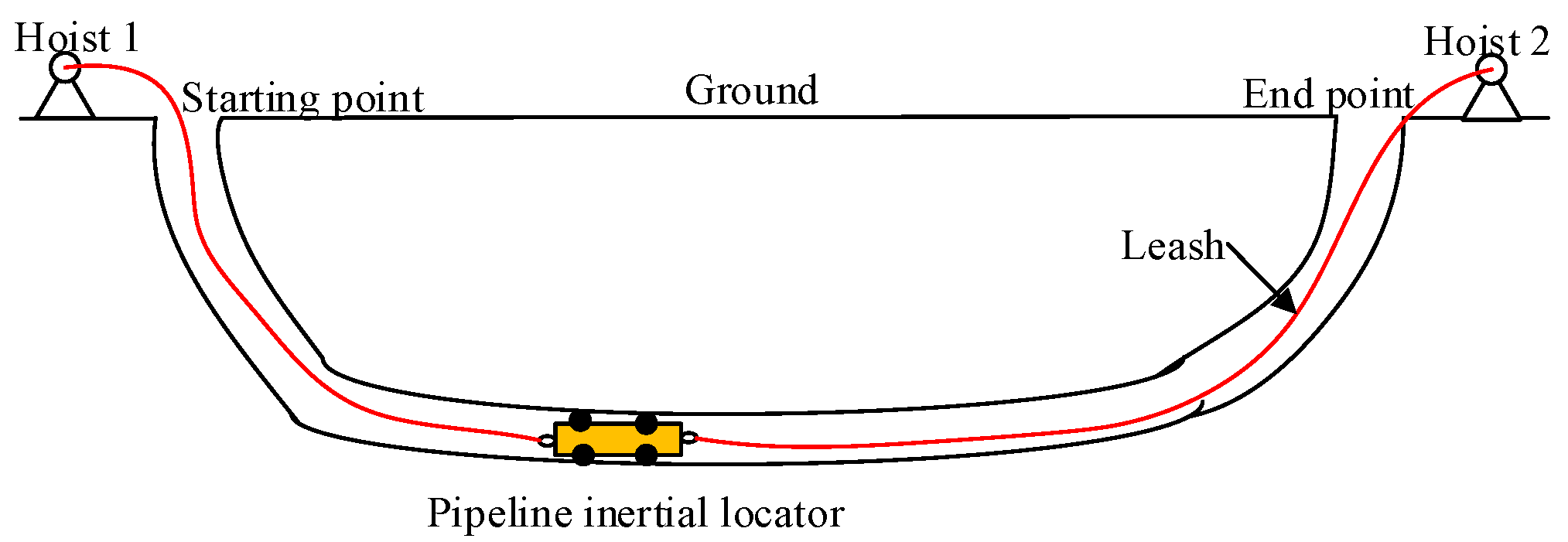
5. Simulation and Experiment

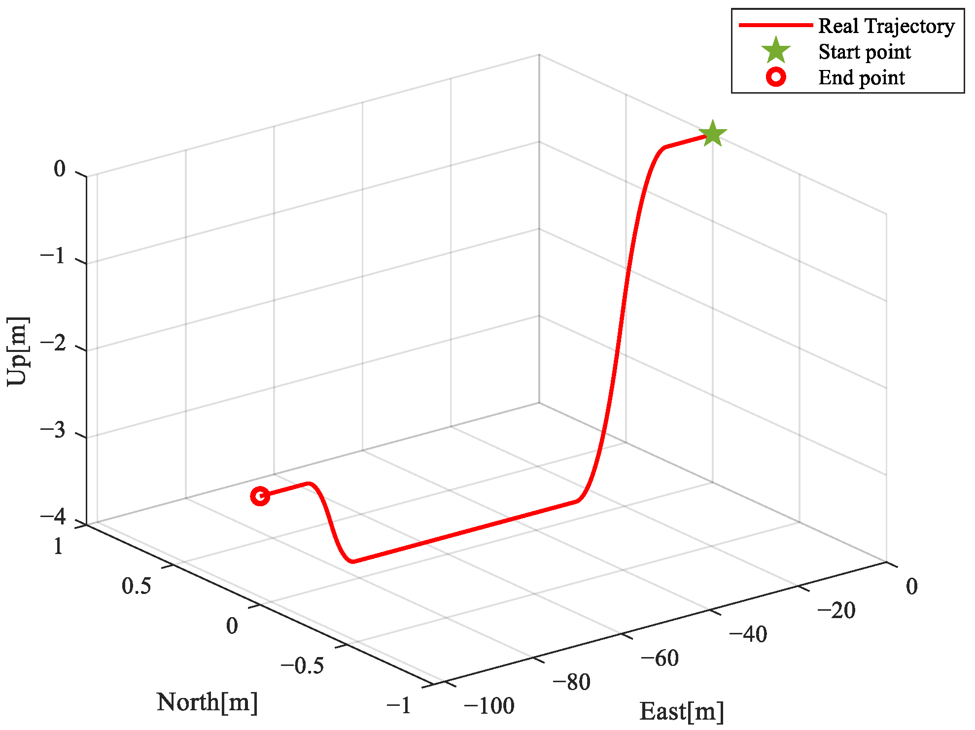
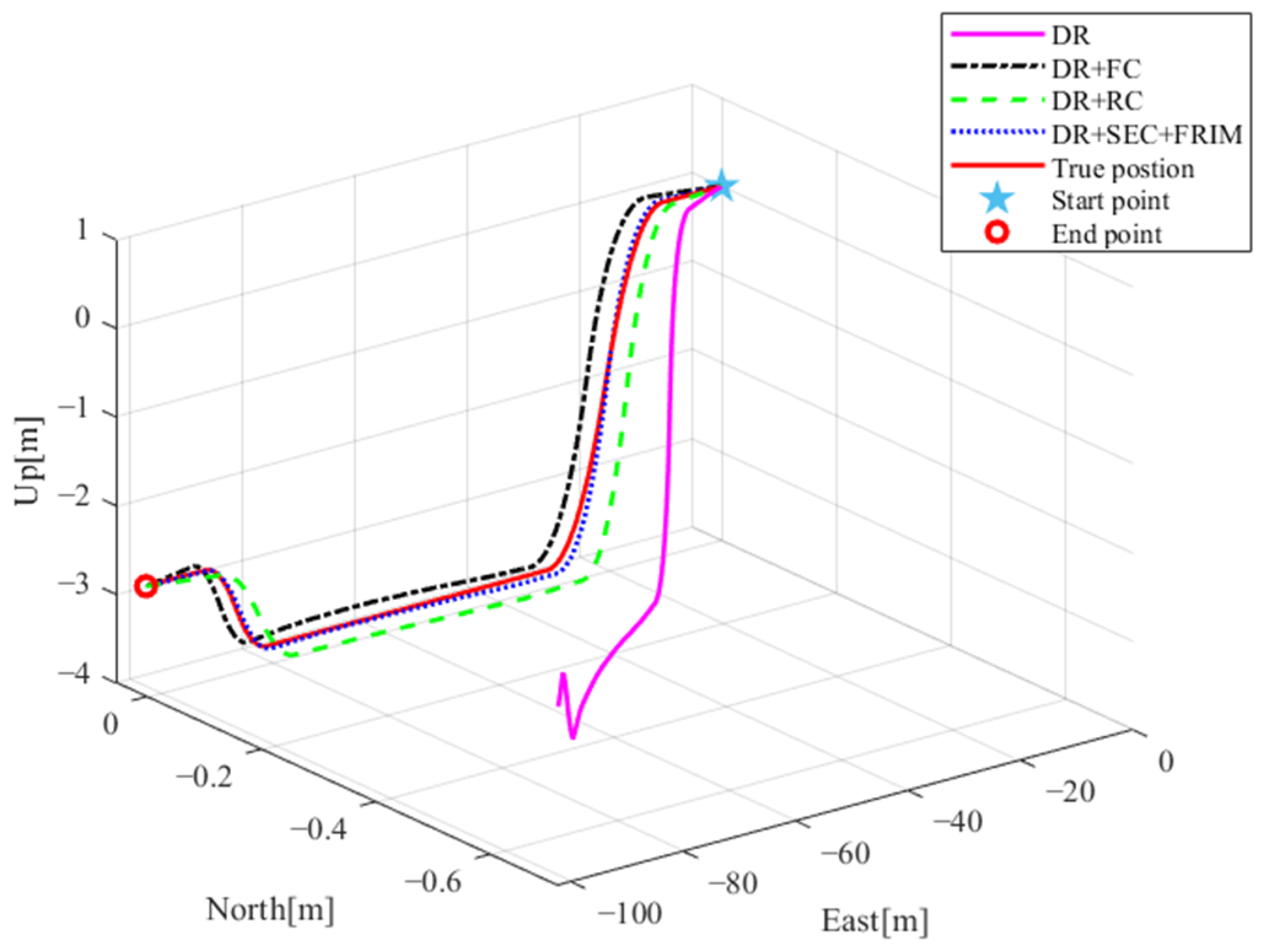
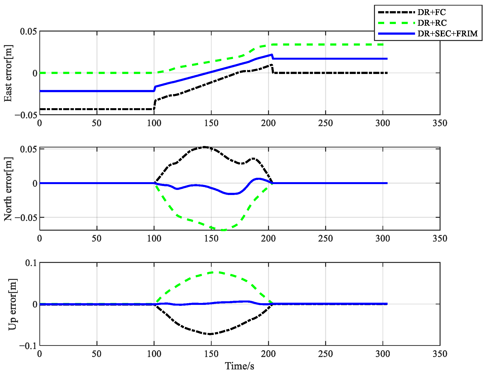
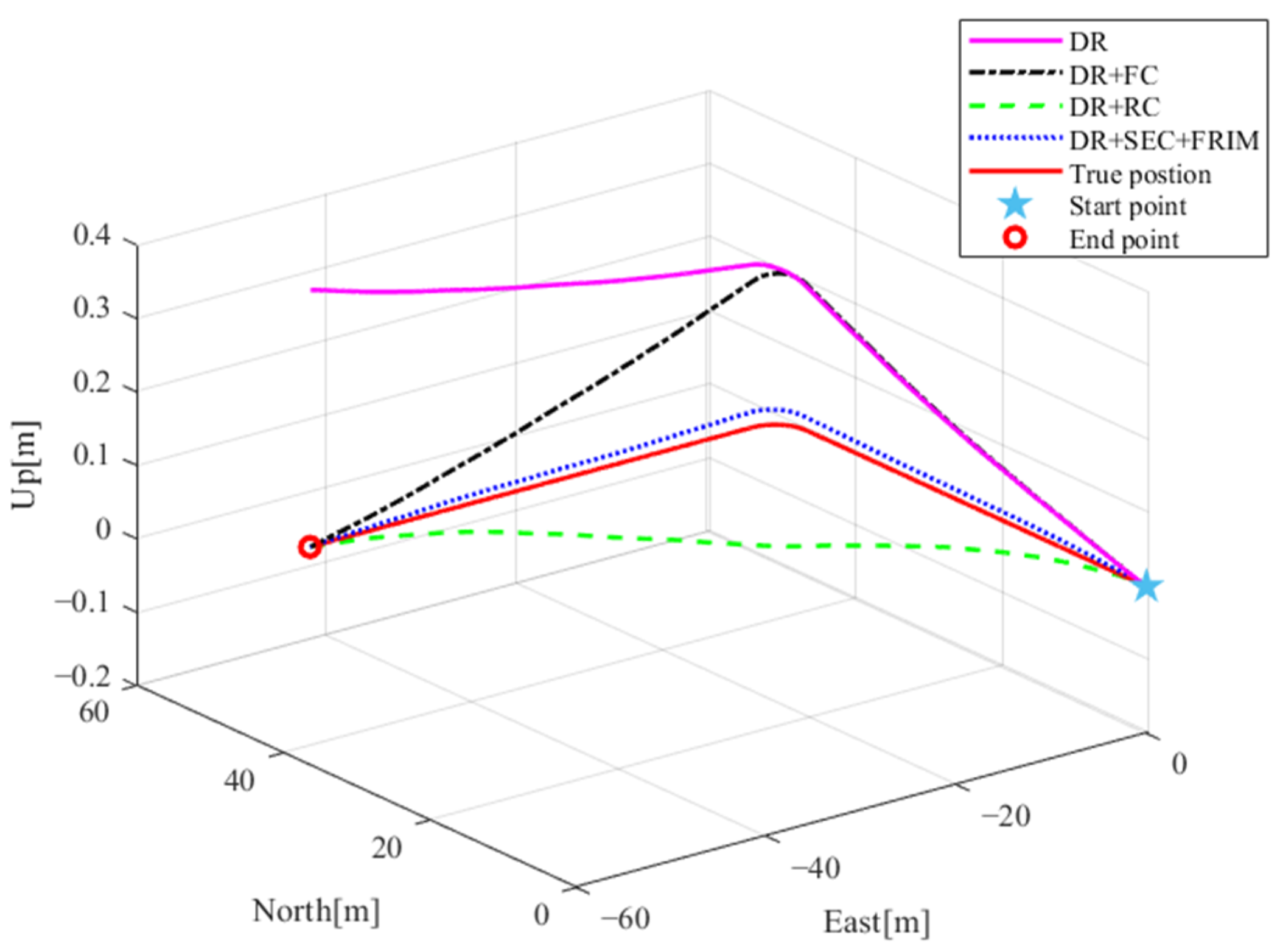
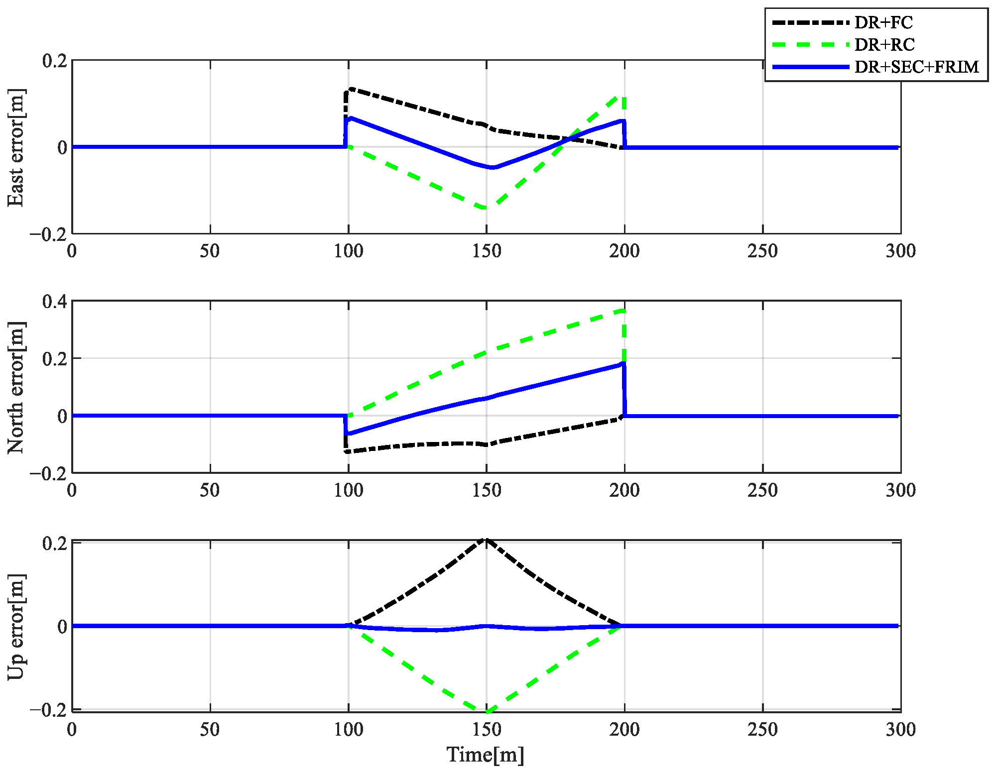
5.1. Simulation Results

The algorithm proposed in this paper based on the start and end point correction and forward and reverse information multiplexing error correction algorithm (SEC + FRIM) is simulated and verified, and the device accuracy settings are shown in

Table 1. Simulation device parameter settings.

Device	Parameter	Value
Gyroscope	Zero Bias (°/h)	10
	Random walk (°/$\sqrt{\mathrm{h}}$)	0.5
Accelerometer	Zero Bias (mg)	1
	Random walk $({\mathrm{m}/\mathrm{s}}^2/\sqrt{\mathrm{h}}$)	0.3
Odometer	Scale Factor	0.9995

:

The positioning error of the proposed algorithm will also increase with the increase in pipeline length. In order to ensure high-precision mapping and positioning at the CM level, the maximum pipeline length applicable to this algorithm is 100 m. The length of the pipeline simulation trajectory is 100 m, and the simulation trajectory diagram is shown in Figure 6:

In order to fully verify the accuracy and effectiveness of the proposed algorithm, the algorithm proposed in this paper was compared with the existing dead reckoning (DR) algorithm, dead reckoning forward endpoint correction (DR + FC) algorithm, and dead reckoning reverse endpoint correction (DR + RC) algorithm for comparative simulation experiments. The comparison results are shown in Figure 7, Figure 8, Figure 9 and Figure 10:

For the above simulation experiment error statistics, the positioning error statistics of different algorithms are shown in

Table 2. Simulation positioning errors of different algorithms for linear pipelines.

Algorithms	Horizontal Maximum Positioning Error (m)	Horizontal Positioning Error RMS (m)	Height Maximum Positioning Error (m)	Height Positioning Error RMS (m)
DR	0.792	0.518	0.551	0.356
DR + FC	0.093	0.045	0.105	0.057
DR + RC	0.183	0.078	0.121	0.051
DR + SEC + FRIM	0.042	0.023	0.005	0.002

and

Table 3. Simulation localization error of 90° bending pipeline with different algorithms.

Algorithms	Horizontal Maximum Positioning Error (m)	Horizontal Positioning Error RMS (m)	Height Maximum Positioning Error (m)	Height Positioning Error RMS (m)
DR	1.380	0.552	0.325	0.250
DR + FC	0.271	0.179	0.086	0.048
DR + RC	0.422	0.182	0.198	0.087
DR + SEC + FRIM	0.187	0.096	0.011	0.009

.

It can be seen from Table 2 that the horizontal positioning error of the algorithm proposed in this paper is within 5 cm, and the height positioning error is within 0.5 cm when using 10°/h MEMS gyroscopes for 100 m pipelines. The positioning accuracy of the proposed algorithm is better than other dead reckoning correction algorithms.

It can be seen from Table 3 that when the length of the simulated pipeline is set to 100 m and the accuracy of the MEMS gyroscope is set to 10°/h, the maximum horizontal positioning error of the 90° curved pipeline is within 20 cm, and the maximum positioning error of the height is within 5 cm. Although the positioning error is larger than that of the straight pipeline, the positioning accuracy of the algorithm is better than other dead reckoning correction algorithms.

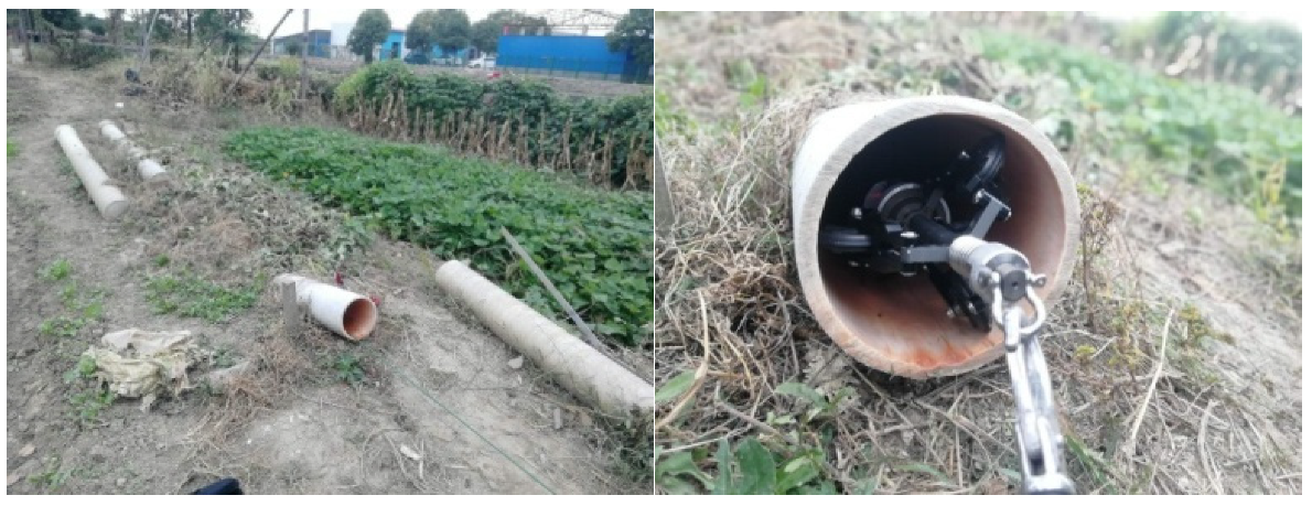
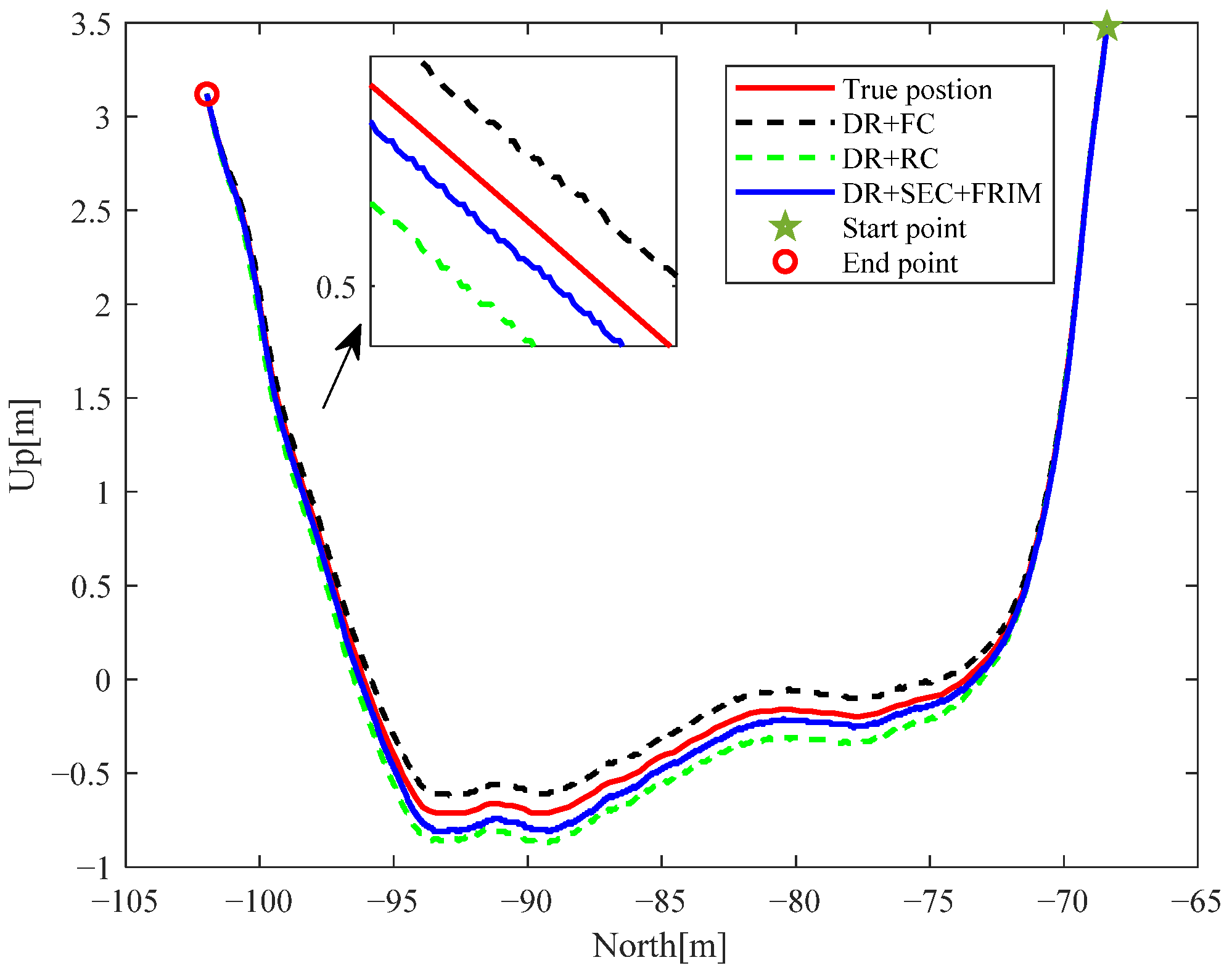
5.2. Experiment Results

In order to better verify and evaluate the effectiveness of the proposed algorithm, the laboratory self-developed pipeline inertial locator was used to conduct the actual measurement experiment. The experimental site is shown in Figure 11.

The pipeline inertial locator developed by the laboratory adopted the STIM300 MEMS gyroscope. The performance indicators of the STIM300 MEMS gyroscope are shown in

Table 4. STIM300 MEMS gyroscope performance index.

Device	Performance	Precision
Gyroscope	Zero bias stability	0.5°/h
	Zero bias stability at all temperatures	10°/h
	Angle random walk	0.2°/$\sqrt{\mathrm{h}}$

below:

The experimental results are shown in Figure 12, Figure 13 and Figure 14 below.

The above Figure 12, Figure 13 and Figure 14 shows the pipeline trajectories solved by different algorithms. The red line is the standard trajectory; the blue line is the trajectory solved by the algorithm proposed in this paper, and the green and black lines are the forward dead reckoning correction algorithm and the reverse dead position, respectively. The trajectory map obtained by the reckoning and correction algorithms is not difficult to see from the above Figure 10, Figure 11 and Figure 12. The trajectory solved by the algorithm proposed in this paper is the closest to the standard trajectory, and the positioning accuracy is the highest. The positioning errors of different algorithms are shown in the following

Table 5. Positional accuracy comparison of different surveying methods.

Different Methods	Horizontal Error (m)	Height Error (m)
DR + FC	0.296	0.125
DR + RC	0.183	0.141
DR + SEC + FRIM	0.074	0.097

and Figure 15:

6. Conclusions

Aiming at the high-precision mapping and positioning of urban, underground, trenchless, short-distance small-diameter pipelines, a dead reckoning algorithm based on start and end point correction and forward and reverse information multiplexing is proposed. Firstly, the correction matrix was constructed by the known start and end point information, and then the corrected forward and reverse trajectory information was fused and averaged to achieve high-precision positioning. Finally, the simulation results show that the maximum horizontal positioning error and the maximum height positioning error for the straight pipeline are both within 5 cm, and the maximum horizontal positioning error for the 90° bend pipeline is within 20 cm, and the maximum height positioning error is within 5 cm. The algorithm effectively solves the problem of rapid accumulation of dead reckoning errors over time, improves positioning accuracy, and has certain practical engineering value.

References

1. Tan, X.; Sun, Z.; Wang, P. On Localization for Magnetic Induction-based Wireless Sensor Networks in Pipeline Environments. In Proceedings of the IEEE International Conference on Communications (ICC), London, UK, 8–12 June 2015; pp. 2780–2785. [Google Scholar]
2. Huang, C.; Peng, F.; Liu, K. Pipeline Inspection Gauge Positioning System Based on Optical Fiber Distributed Acoustic Sensing. IEEE Sens. J. 2021, 21, 25716–25722. [Google Scholar] [CrossRef]
3. Chen, S.L.; Wu, J.L.; Huang, X.J.; Li, J. An accurate localization method for subsea pipelines by using external magnetic fields. Measurement 2019, 147, 106803. [Google Scholar] [CrossRef]
4. Allard, P.; Lavoie, J.-A. Differentiation of 3D Scanners and Their Positioning Method When Applied to Pipeline Integrity; CREAFORM: Lévis, QC, Canada, 2014. [Google Scholar]
5. Maekawa, A.; Takahashi, T.; Tsuji, T.; Noda, M. Noncontact Measurement Method of Vibration Stress Using Optical Displacement Sensors for Piping Systems in Nuclear Power Plants. ASME J. Nucl. Eng. Radiat. Sci. 2015, 1, 31002. [Google Scholar] [CrossRef]
6. Sahli, H. MEMS-Based Aided Inertial Navigation System for Small Diameter Pipelines. Ph.D. Thesis, University of Calgary, Calgary, AB, Canada, 2016. [Google Scholar]
7. Lv, Z.; Wang, G.; Wang, Z.; Zhao, H.; Gao, W. Application of Weld Scar Recognition in Small-Diameter Transportation Pipeline Positioning System. Electronics 2022, 11, 1100. [Google Scholar] [CrossRef]
8. Jin, S.-H.; Ping, Y. Research on the describing of trajectory for subsea pipeline based on Inertial Navigation System. In Proceedings of the 2011 IEEE Power Engineering and Automation Conference, Wuhan, China, 8–9 September 2011; Volume 2, pp. 463–468. [Google Scholar]
9. Wasim, M.; Djukic, M.B. External corrosion of oil and gas pipelines: A review of failure mechanisms and predictive preventions. J. Nat. Gas Sci. Eng. 2022, 100, 104467. [Google Scholar] [CrossRef]
10. Biondi, A.M.; Zhou, J.; Guo, X.; Wu, R.; Tang, Q.; Gandhi, H.; Yu, T.; Gopalan, B.; Hanna, T.; Ivey, J.; et al. Pipeline structural health monitoring using distributed fiber optic sensing textile. Opt. Fiber Technol. 2022, 70, 102876. [Google Scholar] [CrossRef]
11. Al-Masri, W.M.F.; Abdel-Hafez, M.F.; Jaradat, M.A.K. Inertial Navigation System of Pipeline Inspection Gauge. IEEE Trans. Control. Syst. Technol. 2020, 28, 609–616. [Google Scholar] [CrossRef]
12. Niu, X.; Kuang, J.; Chen, Q. Study on the Posibility of the PIG Positioning Using MEMS-based IMU. Chin. J. Sens. Actuators 2016, 29, 40–44. [Google Scholar]
13. Chen, Q.J.; Zhang, Q.; Niu, X.J.; Wang, Y. Positioning Accuracy of a Pipeline Surveying System Based on MEMS IMU and Odometer: Case Study. IEEE Access 2019, 7, 104453–104461. [Google Scholar] [CrossRef]
14. Huang, F.; Sun, L.; Guo, L.; Yang, L.I.; Qian, F. High-accuracy positioning method based on reverse navigation solution in pipeline detection. J. Chin. Inert. Technol. 2018, 26, 435–439. [Google Scholar]
15. Sahli, H.; Moussa, A.; Noureldin, A.; El-Sheimy, N. Small Pipeline Trajectory Estimation Using MEMS Based IMU. In Proceedings of the 27th International Technical Meeting of the Satellite Division of The Institute of Navigation (ION GNSS+ 2014), Tampa, FL, USA, 8–12 September 2014. [Google Scholar]
16. Li, R.; Feng, Q.; Cai, M.; Li, H.; Zhao, X. Measurement of long-distance buried pipeline centerline based on multi-sensor data fusion. Acta Petrol. Sin. 2014, 35, 987–992. [Google Scholar]
17. Zhang, S.; Dubljevic, S. Trajectory determination for pipelines using an inspection robot and pipeline features. Metrol. Meas. Syst. 2021, 28, 439–453. [Google Scholar] [CrossRef]
18. Zhang, P.; Hancock, C.M.; Lau, L.; Roberts, G.W.; de Ligt, H. Low-cost IMU and odometer tightly coupled integration with Robust Kalman filter for underground 3-D pipeline mapping. Measurement 2019, 137, 454–463. [Google Scholar] [CrossRef]
19. Liu, J.; Liu, X.; Yang, W.; Pan, S. Investigating the survey instrument for the underground pipeline with inertial sensor and dead reckoning method. Rev. Sci. Instrum. 2021, 92, 025112. [Google Scholar] [CrossRef] [PubMed]
20. Zhang, B.; Jia, H.G.; Chu, H.R. MEMS-SINS Transfer Alignment Based on UKF. Comput. Simul. 2015, 32, 29–33. [Google Scholar]
21. Lu, J.; Lei, C.; Li, B.A.; Wen, T. Improved calibration of IMU biases in analytic coarse alignment for AHRS. Meas. Sci. Technol. 2016, 27, 075105. [Google Scholar] [CrossRef]
22. Kang, G.; Ren, S.; Chen, X.; Yi, G.; Xu, Z. High precision SINS/OD dead reckoning algorithm considering lever arm effect. In Proceedings of the IECON 2017—43rd Annual Conference of the IEEE Industrial Electronics Society, Beijing, China, 29 October–1 November 2017. [Google Scholar]
23. Chen, Q.; Niu, X.; Kuang, J.; Liu, J.-N. IMU Mounting Angle Calibration for Pipeline Surveying Apparatus. IEEE Trans. Instrum. Meas. 2020, 69, 1765–1774. [Google Scholar] [CrossRef]
24. Wang, Z.G.; Tan, J.; Sun, Z.C. Error Factor and Mathematical Model of Positioning with Odometer Wheel. Adv. Mech. Eng. 2015, 7, 305981. [Google Scholar] [CrossRef] [PubMed]
Figure 1. Principle diagram of dead reckoning.
Electronics 11 02931 g001
Figure 2. Coordinate system definition and schematic diagram of sensor installation.
Electronics 11 02931 g002
Figure 3. Physical map of pipeline inertial locator.
Electronics 11 02931 g003
Figure 4. Schematic diagram of underground short-distance, small-diameter pipeline.
Electronics 11 02931 g004
Figure 5. Schematic diagram of start and end point correction and forward and reverse information multiplexing.
Electronics 11 02931 g005
Figure 6. Real trajectory simulation diagram.
Electronics 11 02931 g006
Figure 7. Comparison of the proposed algorithm and the correction algorithm for others.
Electronics 11 02931 g007
Figure 8. Comparison diagram of trajectory position error calculated by different algorithms.
Electronics 11 02931 g008
Figure 9. Comparison of simulation results of different algorithms for 90° bending pipeline.
Electronics 11 02931 g009
Figure 10. Error diagram of simulation results of different algorithms for 90° bending pipeline.
Electronics 11 02931 g010
Figure 11. Experiment diagram of outfield pipeline measurement.
Electronics 11 02931 g011
Figure 12. Experimental results of three-dimensional positioning of pipelines based on different methods.
Electronics 11 02931 g012
Figure 13. Pipeline height localization results based on different algorithms.
Electronics 11 02931 g013
Figure 14. Pipeline horizontal positioning results based on different algorithms.
Electronics 11 02931 g014
Figure 15. Pipeline positioning error diagram based on different algorithms.
Electronics 11 02931 g015