
Feature Map Analysis-Based Dynamic CNN Pruning and the Acceleration on FPGAs


Abstract
:1. Introduction
- a dynamic method to evaluate the redundancy of filters by observing the intermediate feature map. The evaluation process needs no additional constraints or structures and has good generalization ability.
- implementing the proposed pruned networks on a FPGA and achieving significant acceleration.
2. Related Work
3. Methods
3.1. Preliminary
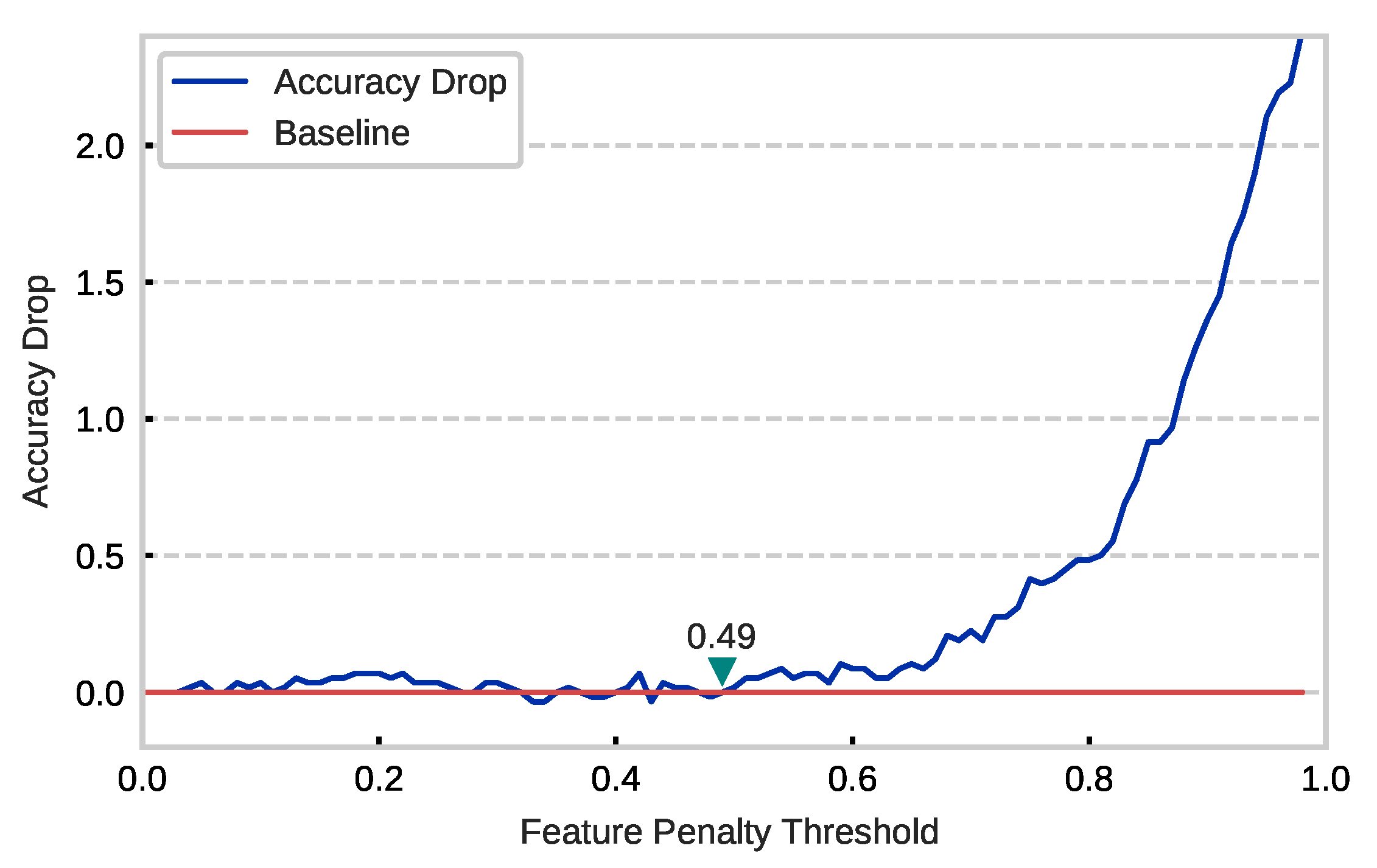
3.2. Redundancy Analysis
3.3. Dynamic Unimportant Filter Identification
| Algorithm 1: Algorithm for dynamic pruning and adjustment of . |
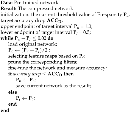 |
4. Experimental
4.1. Experimental Configuration
4.2. Results on Cifar10
4.3. Results on Cifar100
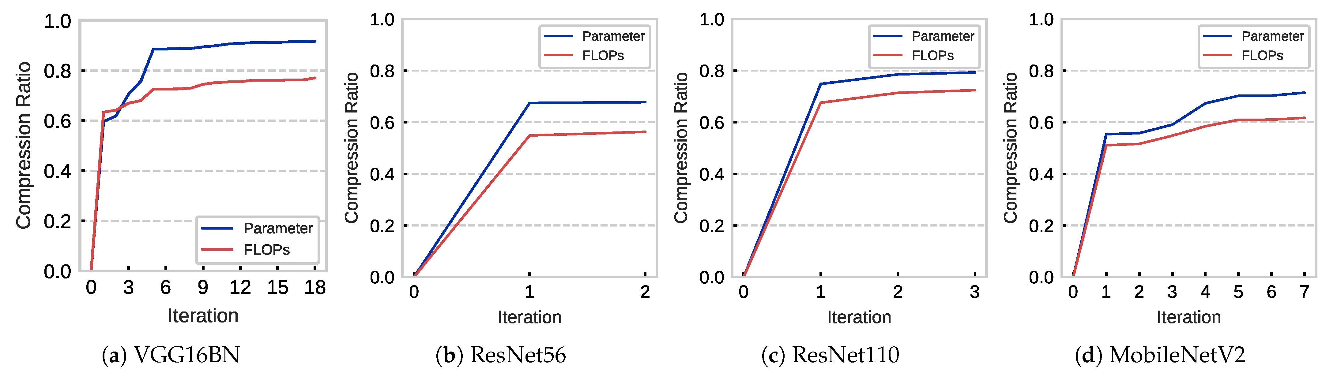
4.4. Analysis
4.5. Implementation on the FPGA
5. Conclusions
Author Contributions
Funding
Institutional Review Board Statement
Informed Consent Statement
Data Availability Statement
Conflicts of Interest
Appendix A

| Abbreviation | Explanation |
|---|---|
| CNN | Convolution Neural Network |
| FLOP | Floating-point operation |
| FPGA | Field-programmable gate array |
| GPU | Graphics processing unit |
| CPU | Central Processing Unit |
| K | Filter kernel size |
| C | Number of input channels |
| The 2D filter applied on the jth output channel | |
| Input feature map | |
| Output feature map | |
| ⊛ | Convolution operator |
| b | Bias |
| En-sparsity | Sparsity obtained by the feature penalty method |
| Threshold value of En-sparsity | |
| Constraint on accuracy drop | |
| Upper endpoint of target interval | |
| Lower endpoint of target interval | |
| Current demarcation point of En-sparsity | |
| DPU | Deep-learning Processing Unit |
| Ours- | Proposed method with |
| method- | A variant of the method |
| AULM | Proposal in the paper [29] |
| Hinge | Proposal in the paper [20] |
| HRank | Proposal in the paper [38] |
| SCP | Proposal in the paper [39] |
| FPGM | Proposal in the paper [40] |
References
- Jiang, W.; Ren, Y.; Liu, Y.; Leng, J. Artificial Neural Networks and Deep Learning Techniques Applied to Radar Target Detection: A Review. Electronics 2022, 11, 156. [Google Scholar] [CrossRef]
- Chen, X.; Liu, L.; Tan, X. Robust Pedestrian Detection Based on Multi-Spectral Image Fusion and Convolutional Neural Networks. Electronics 2022, 11, 1. [Google Scholar] [CrossRef]
- Avazov, K.; Mukhiddinov, M.; Makhmudov, F.; Cho, Y.I. Fire Detection Method in Smart City Environments Using a Deep-Learning-Based Approach. Electronics 2022, 11, 73. [Google Scholar] [CrossRef]
- Krizhevsky, A.; Sutskever, I.; Hinton, G.E. Imagenet classification with deep convolutional neural networks. Adv. Neural Inf. Process. Syst. 2012, 25, 84–90. [Google Scholar] [CrossRef]
- Yue, X.; Li, H.; Fujikawa, Y.; Meng, L. Dynamic Dataset Augmentation for Deep Learning-based Oracle Bone Inscriptions Recognition. J. Comput. Cult. Herit. (JOCCH) 2022. [Google Scholar] [CrossRef]
- Meng, L.; Hirayama, T.; Oyanagi, S. Underwater-drone with panoramic camera for automatic fish recognition based on deep learning. IEEE Access 2018, 6, 17880–17886. [Google Scholar] [CrossRef]
- Paradisa, R.H.; Bustamam, A.; Mangunwardoyo, W.; Victor, A.A.; Yudantha, A.R.; Anki, P. Deep Feature Vectors Concatenation for Eye Disease Detection Using Fundus Image. Electronics 2022, 11, 23. [Google Scholar] [CrossRef]
- Saho, K.; Hayashi, S.; Tsuyama, M.; Meng, L.; Masugi, M. Machine Learning-Based Classification of Human Behaviors and Falls in Restroom via Dual Doppler Radar Measurements. Sensors 2022, 22, 1721. [Google Scholar] [CrossRef] [PubMed]
- Zhou, H.; Alvarez, J.M.; Porikli, F. Less Is More: Towards Compact CNNs. In Computer Vision—ECCV 2016; Springer International Publishing: Berlin/Heidelberg, Germany, 2016; pp. 662–677. [Google Scholar]
- Gong, C.; Chen, Y.; Lu, Y.; Li, T.; Hao, C.; Chen, D. VecQ: Minimal Loss DNN Model Compression With Vectorized Weight Quantization. IEEE Trans. Comput. 2021, 70, 696–710. [Google Scholar] [CrossRef]
- Lin, S.; Ji, R.; Chen, C.; Tao, D.; Luo, J. Holistic CNN Compression via Low-Rank Decomposition with Knowledge Transfer. IEEE Trans. Pattern Anal. Mach. Intell. 2019, 41, 2889–2905. [Google Scholar] [CrossRef] [PubMed]
- Guo, K.; Zeng, S.; Yu, J.; Wang, Y.; Yang, H. [DL] A survey of FPGA-based neural network inference accelerators. ACM Trans. Reconfigurable Technol. Syst. (TRETS) 2019, 12, 1–26. [Google Scholar] [CrossRef]
- Ding, X.; Hao, T.; Tan, J.; Liu, J.; Han, J.; Guo, Y.; Ding, G. ResRep: Lossless CNN Pruning via Decoupling Remembering and Forgetting. In Proceedings of the IEEE/CVF International Conference on Computer Vision (ICCV), Montreal, BC, Canada, 11–17 October 2021; pp. 4510–4520. [Google Scholar]
- Chen, T.; Ji, B.; Ding, T.; Fang, B.; Wang, G.; Zhu, Z.; Liang, L.; Shi, Y.; Yi, S.; Tu, X. Only train once: A one-shot neural network training and pruning framework. Adv. Neural Inf. Process. Syst. 2021, 34, 19637–19651. [Google Scholar]
- Li, B.; Wu, B.; Su, J.; Wang, G. Eagleeye: Fast sub-net evaluation for efficient neural network pruning. In European Conference on Computer Vision; Springer: Berlin/Heidelberg, Germany, 2020; pp. 639–654. [Google Scholar]
- Han, S.; Pool, J.; Tran, J.; Dally, W. Learning both Weights and Connections for Efficient Neural Network. In Advances in Neural Information Processing Systems; Cortes, C., Lawrence, N., Lee, D., Sugiyama, M., Garnett, R., Eds.; Curran Associates, Inc.: New York, NY, USA, 2015; Volume 28. [Google Scholar]
- Molchanov, P.; Tyree, S.; Karras, T.; Aila, T.; Kautz, J. Pruning Convolutional Neural Networks for Resource Efficient Inference. arXiv 2016, arXiv:1611.06440. [Google Scholar]
- Ding, X.; Ding, G.; Han, J.; Tang, S. Auto-balanced filter pruning for efficient convolutional neural networks. In Proceedings of the AAAI Conference on Artificial Intelligence, New Orleans, LA, USA, 2–7 February 2018; Volume 32. [Google Scholar]
- Li, H.; Yue, X.; Wang, Z.; Chai, Z.; Wang, W.; Tomiyama, H.; Meng, L. Optimizing the deep neural networks by layer-wise refined pruning and the acceleration on FPGA. Comput. Intell. Neurosci. 2022, 2022, 8039281. [Google Scholar] [CrossRef]
- Li, Y.; Gu, S.; Mayer, C.; Gool, L.V.; Timofte, R. Group sparsity: The hinge between filter pruning and decomposition for network compression. In Proceedings of the IEEE/CVF Conference on Computer Vision and Pattern Recognition, Seattle, WA, USA, 13–19 June 2020; pp. 8018–8027. [Google Scholar]
- Li, H.; Kadav, A.; Durdanovic, I.; Samet, H.; Graf, H.P. Pruning Filters for Efficient ConvNets. arXiv 2016, arXiv:1608.08710. [Google Scholar]
- Luo, J.H.; Wu, J.; Lin, W. ThiNet: A Filter Level Pruning Method for Deep Neural Network Compression. In Proceedings of the IEEE International Conference on Computer Vision (ICCV), Venice, Italy, 22–29 October 2017. [Google Scholar]
- He, Y.; Kang, G.; Dong, X.; Fu, Y.; Yang, Y. Soft Filter Pruning for Accelerating Deep Convolutional Neural Networks. arXiv 2018, arXiv:1808.06866. [Google Scholar]
- Molchanov, D.; Ashukha, A.; Vetrov, D. Variational dropout sparsifies deep neural networks. arXiv 2017, arXiv:1701.05369. [Google Scholar]
- Liu, Z.; Li, J.; Shen, Z.; Huang, G.; Yan, S.; Zhang, C. Learning Efficient Convolutional Networks Through Network Slimming. In Proceedings of the IEEE International Conference on Computer Vision (ICCV), Venice, Italy, 22–29 October 2017. [Google Scholar]
- Zhao, C.; Ni, B.; Zhang, J.; Zhao, Q.; Zhang, W.; Tian, Q. Variational Convolutional Neural Network Pruning. In Proceedings of the IEEE/CVF Conference on Computer Vision and Pattern Recognition (CVPR), Long Beach, CA, USA, 15–20 June 2019. [Google Scholar]
- Ye, J.; Lu, X.; Lin, Z.; Wang, J.Z. Rethinking the Smaller-Norm-Less-Informative Assumption in Channel Pruning of Convolution Layers. arXiv 2018, arXiv:1802.00124. [Google Scholar]
- Huang, Z.; Wang, N. Data-Driven Sparse Structure Selection for Deep Neural Networks. In Proceedings of the European Conference on Computer Vision (ECCV), Munich, Germany, 8–14 September 2018. [Google Scholar]
- Lin, S.; Ji, R.; Li, Y.; Deng, C.; Li, X. Toward compact convnets via structure-sparsity regularized filter pruning. IEEE Trans. Neural Networks Learn. Syst. 2019, 31, 574–588. [Google Scholar] [CrossRef]
- Dong, X.; Huang, J.; Yang, Y.; Yan, S. More is less: A more complicated network with less inference complexity. In Proceedings of the IEEE Conference on Computer Vision and Pattern Recognition, Honolulu, HI, USA, 21–26 July 2017; pp. 5840–5848. [Google Scholar]
- Ding, X.; Chen, H.; Zhang, X.; Huang, K.; Han, J.; Ding, G. Re-parameterizing Your Optimizers rather than Architectures. arXiv 2022, arXiv:2205.15242. [Google Scholar]
- Li, H.; Wang, Z.; Yue, X.; Wang, W.; Tomiyama, H.; Meng, L. An architecture-level analysis on deep learning models for low-impact computations. Artif. Intell. Rev. 2022, 1–40. [Google Scholar] [CrossRef]
- Simonyan, K.; Zisserman, A. Very Deep Convolutional Networks for Large-Scale Image Recognition. arXiv 2014, arXiv:1409.1556. [Google Scholar]
- He, K.; Zhang, X.; Ren, S.; Sun, J. Deep residual learning for image recognition. In Proceedings of the IEEE conference on computer vision and pattern recognition, Las Vegas, NV, USA, 27–30 June 2016; pp. 770–778. [Google Scholar]
- Sandler, M.; Howard, A.; Zhu, M.; Zhmoginov, A.; Chen, L.C. Mobilenetv2: Inverted residuals and linear bottlenecks. In Proceedings of the IEEE conference on computer vision and pattern recognition, Salt Lake City, UT, USA, 18–23 June 2018; pp. 4510–4520. [Google Scholar]
- CIFAR-10 and CIFAR-100 Datasets. Available online: https://www.cs.toronto.edu/~kriz/cifar.html (accessed on 3 October 2021).
- Loshchilov, I.; Hutter, F. SGDR: Stochastic Gradient Descent with Warm Restarts. arXiv 2016, arXiv:1608.03983. [Google Scholar]
- Lin, M.; Ji, R.; Wang, Y.; Zhang, Y.; Zhang, B.; Tian, Y.; Shao, L. HRank: Filter Pruning Using High-Rank Feature Map. In Proceedings of the IEEE/CVF Conference on Computer Vision and Pattern Recognition (CVPR), Seattle, WA, USA, 13–19 June 2020. [Google Scholar]
- Kang, M.; Han, B. Operation-aware soft channel pruning using differentiable masks. arXiv 2020, arXiv:2007.03938. [Google Scholar]
- He, Y.; Liu, P.; Wang, Z.; Hu, Z.; Yang, Y. Filter pruning via geometric median for deep convolutional neural networks acceleration. In Proceedings of the IEEE/CVF Conference on Computer Vision and Pattern Recognition, Long Beach, CA, USA, 15–20 June 2019; pp. 4340–4349. [Google Scholar]
- VitisAI Develop Environment. Available online: https://japan.xilinx.com/products/design-tools/vitis/vitis-ai.html (accessed on 2 March 2022).
- Hubara, I.; Nahshan, Y.; Hanani, Y.; Banner, R.; Soudry, D. Improving Post Training Neural Quantization: Layer-wise Calibration and Integer Programming. arXiv 2020, arXiv:2006.10518. [Google Scholar]
- Yue, X.; Li, H.; Shimizu, M.; Kawamura, S.; Meng, L. YOLO-GD: A Deep Learning-Based Object Detection Algorithm for Empty-Dish Recycling Robots. Machines 2022, 10, 294. [Google Scholar] [CrossRef]
- Xue, X.; Zhou, D.; Chen, F.; Yu, X.; Feng, Z.; Duan, Y.; Meng, L.; Zhang, M. From SOA to VOA: A Shift in Understanding the Operation and Evolution of Service Ecosystem. IEEE Trans. Serv. Comput. 2021, 1-1. [Google Scholar] [CrossRef]


| Dataset | Model | Top-1 (%) | FLOPs (M) | Param. (M) |
|---|---|---|---|---|
| Cifar10 | VGG16BN | 94.14 | 314.03 | 14.73 |
| ResNet56 | 94.45 | 126.56 | 0.85 | |
| ResNet110 | 94.49 | 254.99 | 1.73 | |
| MobileNetV2 | 92.78 | 25.55 | 2.24 | |
| Cifar100 | VGG16BN | 73.47 | 314.08 | 14.77 |
| ResNet56 | 71.61 | 126.56 | 0.86 | |
| ResNet110 | 73.72 | 255.00 | 1.73 | |
| MobileNetV2 | 67.01 | 25.67 | 2.35 |
| Model | Pruned Top-1 (%) | Pruned FLOPs (M) | Pruned Param. (M) | Top-1 ↓ (%) | FLOPs ↓ (%) | Param. ↓ (%) | |
|---|---|---|---|---|---|---|---|
| VGG16BN | 1% | 93.60 | 71.92 | 1.22 | 0.54 | 77.10 | 91.72 |
| 2% | 92.44 | 34.18 | 0.43 | 1.70 | 89.12 | 97.09 | |
| 3% | 91.39 | 43.00 | 0.52 | 2.75 | 86.31 | 96.45 | |
| ResNet56 | 1% | 93.54 | 55.34 | 0.27 | 0.91 | 56.27 | 67.77 |
| 2% | 92.54 | 34.49 | 0.15 | 1.95 | 72.75 | 82.63 | |
| 3% | 91.83 | 32.88 | 0.12 | 2.62 | 74.02 | 86.27 | |
| ResNet110 | 1% | 93.94 | 70.31 | 0.36 | 0.76 | 72.43 | 79.28 |
| 2% | 92.95 | 46.90 | 0.21 | 1.75 | 81.61 | 87.64 | |
| 3% | 91.76 | 34.37 | 0.13 | 2.94 | 86.52 | 92.38 | |
| MobileNetV2 | 1% | 91.87 | 9.78 | 0.64 | 0.91 | 61.72 | 71.47 |
| 2% | 90.82 | 8.80 | 0.54 | 1.96 | 65.56 | 75.70 | |
| 3% | 89.84 | 7.78 | 0.56 | 2.94 | 69.55 | 75.16 |
| Model | Pruned Top-1 (%) | Pruned FLOPs (M) | Pruned Param. (M) | Top-1 ↓ (%) | FLOPs ↓ (%) | Param. ↓ (%) | |
|---|---|---|---|---|---|---|---|
| VGG16BN | 1% | 72.63 | 149.57 | 2.52 | 0.84 | 52.38 | 82.94 |
| 2% | 71.81 | 115.05 | 1.47 | 1.66 | 63.37 | 90.05 | |
| 3% | 70.55 | 119.54 | 1.26 | 2.92 | 61.94 | 91.47 | |
| ResNet56 | 1% | 70.80 | 81.95 | 0.49 | 0.81 | 35.25 | 43.02 |
| 2% | 69.72 | 64.71 | 0.36 | 1.89 | 48.87 | 58.35 | |
| 3% | 68.76 | 55.47 | 0.30 | 2.85 | 56.17 | 64.75 | |
| ResNet110 | 1% | 73.07 | 159.64 | 0.90 | 0.65 | 37.40 | 48.11 |
| 2% | 72.33 | 128.53 | 0.70 | 1.39 | 49.60 | 59.62 | |
| 3% | 70.78 | 100.24 | 0.44 | 2.94 | 60.69 | 74.49 | |
| MobileNetV2 | 1% | 66.04 | 8.09 | 0.68 | 0.97 | 68.48 | 70.92 |
| 2% | 65.10 | 8.26 | 0.67 | 1.91 | 67.82 | 71.50 | |
| 3% | 64.03 | 7.77 | 0.65 | 2.98 | 69.73 | 72.55 |
| Model | Method | Pruned Top-1 (%) | FLOP ↓ (%) | Param. ↓ (%) |
|---|---|---|---|---|
| ResNet56 | HRank | 93.17 | 50.00 | 42.40 |
| SCP | 93.23 | 51.50 | 48.47 | |
| FPGM | 93.49 | 52.60 | - | |
| ours-1% | 93.54 | 56.27 | 67.77 | |
| Hinge | 93.69 | 50.00 | 51.27 | |
| HRank- | 90.72 | 74.10 | 68.10 | |
| ours-3% | 91.83 | 74.02 | 86.27 | |
| ours-2% | 92.54 | 72.75 | 82.63 | |
| Hinge- | 92.65 | 76.00 | 79.20 | |
| ResNet110 | HRank | 93.36 | 58.20 | 59.20 |
| FPGM | 93.74 | 52.30 | - | |
| ours-1% | 93.94 | 72.43 | 79.28 | |
| HRank- | 92.65 | 68.60 | 68.70 | |
| ours-2% | 92.95 | 81.61 | 84.64 |
| Model | Cifar10 | Cifar100 | ||||
|---|---|---|---|---|---|---|
| CPU | GPU | FPGA | CPU | GPU | FPGA | |
| VGG16BN | 2.42 | 0.87 | 2.44 | 2.59 | 0.89 | 2.45 |
| ResNet56 | 3.22 | 1.55 | 0.68 | 3.29 | 1.57 | 0.68 |
| ResNet110 | 6.77 | 3.02 | 1.22 | 6.15 | 3.04 | 1.23 |
| MobileNetV2 | 3.54 | 1.20 | 1.49 | 2.96 | 1.19 | 1.51 |
| Model | Cifar10 | Cifar100 | |||||
|---|---|---|---|---|---|---|---|
| Top-1 (%) | Time (ms) | Top-1 ↓ (%) | Top-1 (%) | Time (ms) | Top-1 ↓(%) | ||
| VGG16BN | 1% | 93.59 | 0.47 | 0.55 | 72.31 | 0.704 | 1.16 |
| 2% | 92.21 | 0.32 | 1.93 | 71.58 | 0.556 | 1.89 | |
| 3% | 91.30 | 0.34 | 2.84 | 70.41 | 0.552 | 3.06 | |
| ResNet56 | 1% | 93.36 | 0.52 | 1.09 | 69.73 | 0.608 | 1.88 |
| 2% | 92.05 | 0.41 | 2.40 | 68.43 | 0.562 | 3.18 | |
| 3% | 91.40 | 0.41 | 3.05 | 68.08 | 0.536 | 3.53 | |
| ResNet110 | 1% | 93.50 | 0.74 | 0.99 | 71.68 | 1.06 | 2.04 |
| 2% | 92.57 | 0.65 | 1.92 | 71.10 | 0.98 | 2.62 | |
| 3% | 91.60 | 0.55 | 2.89 | 68.97 | 0.892 | 4.75 | |
| MobileNetV2 | 1% | 91.66 | 0.59 | 1.12 | 65.30 | 0.623 | 1.71 |
| 2% | 90.42 | 0.55 | 2.36 | 64.62 | 0.628 | 2.39 | |
| 3% | 89.43 | 0.51 | 3.35 | 63.21 | 0.607 | 3.8 | |
| Model | Cifar10 | Cifar100 | |||||
|---|---|---|---|---|---|---|---|
| vs. CPU ↓ (%) | vs. GPU ↓ (%) | vs. FPGA ↓ (%) | vs. CPU ↓ (%) | vs. GPU ↓ (%) | vs. FPGA ↓ (%) | ||
| VGG16BN | 1% | 80.47 | 45.47 | 80.66 | 72.85 | 21.12 | 71.24 |
| 2% | 86.97 | 63.61 | 87.09 | 78.56 | 37.70 | 77.29 | |
| 3% | 86.14 | 61.30 | 86.27 | 78.71 | 38.15 | 77.45 | |
| ResNet56 | 1% | 83.82 | 66.41 | 22.81 | 81.54 | 61.37 | 10.98 |
| 2% | 87.33 | 73.70 | 39.56 | 82.94 | 64.29 | 17.72 | |
| 3% | 87.21 | 73.44 | 38.96 | 83.73 | 65.94 | 21.52 | |
| ResNet110 | 1% | 89.10 | 75.53 | 39.56 | 82.77 | 65.12 | 13.68 |
| 2% | 90.37 | 78.38 | 46.60 | 84.07 | 67.75 | 20.20 | |
| 3% | 91.92 | 81.86 | 55.20 | 85.50 | 70.65 | 27.36 | |
| MobileNetV2 | 1% | 83.28 | 50.90 | 60.20 | 78.98 | 47.56 | 58.63 |
| 2% | 84.36 | 54.06 | 62.76 | 78.81 | 47.14 | 58.30 | |
| 3% | 85.63 | 57.80 | 65.79 | 79.52 | 48.91 | 59.69 | |
Publisher’s Note: MDPI stays neutral with regard to jurisdictional claims in published maps and institutional affiliations. |
© 2022 by the authors. Licensee MDPI, Basel, Switzerland. This article is an open access article distributed under the terms and conditions of the Creative Commons Attribution (CC BY) license (https://creativecommons.org/licenses/by/4.0/).
Share and Cite
Li, Q.; Li, H.; Meng, L. Feature Map Analysis-Based Dynamic CNN Pruning and the Acceleration on FPGAs. Electronics 2022, 11, 2887. https://doi.org/10.3390/electronics11182887
Li Q, Li H, Meng L. Feature Map Analysis-Based Dynamic CNN Pruning and the Acceleration on FPGAs. Electronics. 2022; 11(18):2887. https://doi.org/10.3390/electronics11182887
Chicago/Turabian StyleLi, Qi, Hengyi Li, and Lin Meng. 2022. "Feature Map Analysis-Based Dynamic CNN Pruning and the Acceleration on FPGAs" Electronics 11, no. 18: 2887. https://doi.org/10.3390/electronics11182887
APA StyleLi, Q., Li, H., & Meng, L. (2022). Feature Map Analysis-Based Dynamic CNN Pruning and the Acceleration on FPGAs. Electronics, 11(18), 2887. https://doi.org/10.3390/electronics11182887