E-Commerce Sales Revenues Forecasting by Means of Dynamically Designing, Developing and Validating a Directed Acyclic Graph (DAG) Network for Deep Learning

Abstract

As the digitalization process has become more and more important in our daily lives, during recent decades e-commerce has greatly increased in popularity, becoming increasingly used, therefore representing an extremely convenient alternative to traditional stores. In order to develop and maintain profitable businesses, traders need accurate forecasts concerning their future sales, a very difficult task considering that these are influenced by a wide variety of factors. This paper proposes a novel e-commerce sales forecasting method that dynamically builds a Directed Acyclic Graph Neural Network (DAGNN) for Deep Learning architecture. This will allow for long-term, fine-grained forecasts of daily sales revenue, refined up to the level of product categories. The developed forecasting method provides the e-commerce store owner an accurate forecasting tool for predicting the sales of each category of products for up to three months ahead. The method offers a high degree of scalability and generalization capability due to the dynamically incremental way in which the constituent elements of the DAGNN’s architecture are obtained. In addition, the proposed method achieves an efficient use of data by combining the numerous advantages of its constituent layers, registering very good performance metrics and processing times. The proposed method can be generalized and applied to forecast the sales for up to three months ahead in the case of other e-commerce stores, including large e-commerce businesses.

1. Introduction

In recent years, the undeniable advantages of e-commerce, as well as the growing needs of customers have led to its worldwide development and expansion. Among these advantages is the fact that an e-commerce business does not face the limitations of a physical store in what concerns the existence of a physical location: the owners of online stores are not tied to a specific fixed location, they only need a computer (a laptop, a tablet, or even a smartphone) and an internet connection to manage their businesses. In addition to this, in contrast to a physical store that has its activity limited to a certain operating schedule, the e-commerce store remains open 24 h a day, 7 days a week, this being an excellent opportunity for both the traders and buyers. Moreover, an e-commerce business has significantly lower operating costs than traditional stores [1], lower costs for the physical location [2], a reduced number of hired and paid employees [3]. Therefore, conducting and maintaining an e-commerce business has many benefits [4,5].

An important advantage of e-commerce-based businesses is the automatic management of inventory, through the use of online electronic tools, which brings e-commerce companies significant reductions in inventory and operating costs compared to physical, classic stores [6]. The owner of an e-commerce company can collect data regarding its customers to ensure that the company is targeting the right people to buy its products, leading to a proper marketing strategy: the customers are informed by appropriate, timely emails about campaigns, discounts, improvements, deals, and recent updates that have appeared and might be of interest to them [7]. This allows e-commerce companies to fulfill the needs of a large number of customers in a relatively short time, which makes it easier for them to build and maintain mutually beneficial, long-term relationships. In every type of commerce, including e-commerce, obtaining reliable and accurate sales revenue forecasts is an essential factor that influences to a large extent the prosperity of the business [8,9,10].

Accurate sales revenue estimates help sales managers to allocate resources efficiently, to estimate the income and plan investments, to identify and manage potential issues, to plan general objectives of the business, and especially to improve the decision-making process in view of business development. In this context, a series of papers from the scientific literature have proposed various sales revenues forecasting methods [2,4,5,8,9,11] that range from single [4,6,12] to hybrid [9,13] methods. Important factors to consider include the overall health of the economy, as well as sector-specific trends. For example, if the overall economy is experiencing a downturn, it is likely that e-commerce sales will also decline. By taking into account a variety of internal and external factors, businesses can develop a more accurate picture regarding their future sales. This information can then be used to make informed decisions about resource allocation, marketing campaigns, and inventory management. By accurately forecasting sales, businesses can improve their decision-making and increase their chances of success.

In this paper, in order to fulfill the requirements of our contractor, an owner of an e-commerce store that needs long-term fine-grained forecasts of daily sales revenues refined up to the level of product categories, we have designed, developed and validated an e-commerce sales forecasting method that dynamically builds a Directed Acyclic Graph Neural Network (DAGNN) for Deep Learning architecture. The contractor has been operating in Romania since 2010 and is selling 3 categories of products. The first category contains electric and electronic products, the second category comprises children’s items, toys, party supplies, and a bookstore (including e-books) and stationery products, while the third category comprises personal and health care items, including food supplements. Most of the specific activities of maintenance, updating the involved software components, managing stocks, and adding promotions, are performed remotely, online, by electronic means, which does not affect the operation of the store except for short periods of time (a few hours at most, once a week or even more rarely), in certain particular cases.

The remaining sections of the paper are: Section 2, “Literature Review”, which presents a series of recent papers from the scientific literature targeting various sales revenues forecasting methods; Section 3, highlighting the “Contributions of the Paper”; Section 4 that presents the “Background” of the targeted subject; Section 5, “Materials and Methods”, within which there are depicted the most important concepts that have been used in developing the forecasting approach, along with a detailed presentation of the stages and steps of the method, synthetized afterwards in a flowchart diagram; Section 6, entitled “Results”, depicts the main outcomes registered after having applied the developed steps and stages of the methodology and afterwards, Section 7, “Discussion” highlights the most relevant findings and their meaning, along with arguments regarding the fact that the knowledge gap identified in the “Introduction” section has been covered by the devised study, and the obtained results are analyzed, interpreted and compared to other ones from the scientific literature; and Section 8, entitled “Conclusions”, emphasizes the most important outcomes of this paper, along with the limitations of the devised study and research directions for future works.

2. Literature Review

Among the most important citing criteria considered when choosing the referenced papers were the relevance of the approached topic in the context of our research, the visibility of the respective article in the scientific literature (as highlighted by its number of citations), the actuality of the cited studies, considering the date of their publication. The purpose of the conducted literature review is to contextualize the results obtained within the research conducted in this paper with a view to identify and target a real need, a gap that exists in the current body of knowledge, which is being addressed by our study.

Within the scientific paper [14], Bandara et al. propose a prediction method based on a Long Short-Term Memory (LSTM) network in order to obtain reliable sales demand forecasts in e-commerce. The authors evaluate the forecasting framework on two datasets collected from an American multinational retail corporation that operates a chain of hypermarkets. The forecasting accuracy is evaluated through the means of a modified version of the Mean Absolute Percentage Error (mMAPE). Finally, the authors compare four variants of their developed approach to a series of univariate forecasting techniques, such as Exponentially Weighted Moving Average (EWMA), Exponential Smoothing (ETS), Autoregressive Integrated Moving Average (ARIMA), Prophet, Naïve, Naïve Seasonal, and therefore remark that their devised approach offers superior results.

Acknowledging the importance that an accurate sales prediction exerts in e-commerce, in the scientific article [15], Ji et al. develop a prediction method based on machine learning techniques. Therefore, they have proposed a three-stage eXtreme Gradient Boosting (XGBoost) forecasting model (entitled C-A-XGBoost). Using real datasets registered on a cross-border e-commerce platform, the authors have compared their obtained results to the ones provided by other models, such as ARIMA, XGBoost, a model based on the clustering and XGBoost (C-XGBoost), and a model that combines the ARIMA with XGBoost (A-XGBoost). Using the Mean Sum Error (ME), MSE, Root Mean Squared Error (RMSE) and the Mean Absolute Error (MAE) as performance metrics, the authors conclude that their developed model outperforms the other four ones.

Within the scientific paper [5], Kharfan et al. put forward a machine-learning approach designed to forecast the demand in the case of products for which historical data are not available and that have been recently launched on an e-commerce platform. The developed model consists of three steps that deal with clustering, classification and finally, prediction. Each of these three steps is developed making use of various techniques that are afterwards benchmarked in order to establish the best method. Therefore, the first step has employed the t-Distributed Stochastic Neighbor Embedding (t-SNE) algorithm and k-means clustering; in the second step, the authors have tested the classification trees, Random Forest (RF) and Support Vector Machine (SVM) in order to identify the best performing one; in the third step, the algorithms of regression trees, k-NN, linear regression (LR), RF and neural networks have been tested. The proposed methodology has been used on a real dataset provided by an e-commerce United States company specialized in clothing and footwear sales in order to obtain a demand forecasting for the newly launched products that do not have historical data available. The authors compute as performance metrics the Absolute Forecast Error (AFE), Absolute Forecast Percentage Error (APE), Weighted Mean Absolute Percentage Error (WMAPE), Forecast Percentage Error (PE), Weighted Mean Percentage Error (WMPE), and in this way, the authors have identified the best method that should be used in each step of the developed model.

In the paper [6], Pan et al. present a CNN approach useful in sales forecasting in the case of e-commerce activities, by mining specific data. The authors remark that in contrast to the traditional data mining techniques, the CNN approach is able to use in an efficient way large amounts of data and automatically extract features from time series. The validity of the developed approach is confirmed using a real dataset. The authors have made use of MSE as a performance metric and compared the performance registered by their approach to the one of other methods from the scientific literature, such as a CNN version in which the weights are adjusted, a single CNN method, an ARIMA algorithm, an algorithm from the scientific literature based on Gaussian Process Regression (GPR) along with Kernel Ridge Regression (KRR) and a Deep Neural Network (DNN) approach. Finally, the authors conclude that their developed approach offers an improved, more accurate sales forecast.

In the article [13], Weytjens et al. firstly remark that an accurate cash flow forecasting helps and improves the capital’s allocation for a wide range of firms, preventing other ones from running out of cash. Targeting e-commerce companies and other firms that have an increased number of customers and transactions, the authors have approached a subject regarding the forecasting of the “Accounts Receivable Cash Flows (ARCF)”. Starting from an analysis of existing forecasting methods, such as ARIMA or Prophet, the authors propose an approach based on neural networks, considering Multi-Layered Perceptron (MLP) and Long-Short-Term Memory (LSTM) ANNs. Using a dataset retrieved from a German company and based on computing as performance metrics the MSE and the “Interest Opportunity Cost (IOC)”, the authors compare ARIMA, Prophet, and the two DL approaches developed within their paper, concluding that the developed methods offer an increased level of flexibility and accuracy.

Acknowledging the importance of sales forecasting in managing e-commerce enterprises and in highlighting future sales trends, within the scientific paper [16], Liu et al. propose a model that uses historical sales and establishes common characteristics among them, by making use of a time series model. The developed approach predicts the sales inventory for a certain type of products. Afterwards, in order to improve the forecasting accuracy and the reliability of the developed model, the authors introduce external datasets and a qualitative analysis of data by means of a Hidden Markov Model (HMM). Using a real e-commerce dataset along with a meteorological dataset provided by the China Weather Network, the authors perform a qualitative analysis of the forecast based on an analysis of the predictive vectors of the HMM in order to confirm the usefulness of the Hidden Markov approach in attaining a qualitative prediction.

In a recent paper, Qi et al. propose a hybrid sales volume forecasting approach designed for e-commerce, based on “Long Short-Term Memory with Particle Swam Optimization (LSTM-PSO)” [9]. In order to obtain the most suitable configuration within the developed approach, the authors make use of a Particle Swam Optimization (PSO) metaheuristic method. Using real datasets provided by an e-commerce company, along with publicly available ones, the authors assess the effectiveness of the devised approach by comparing it with 9 other ones, namely LR, SVM for regression, MLP, M5P, RF, K-Nearest Neighbor (KNN), ARIMA, Transfer Learning (TL) and Recurrent Neural Network (RNN) models. The performance metrics computed and compared within the study are MAE, RMSE, Relative Absolute Error (RAE), Root Relative Squared Error (RRSE). The obtained results emphasize the fact that the developed approach attained a very good prediction accuracy, consequently proving its usefulness.

Shih et al. propose in [1] a hybrid forecasting approach for the goods demand in the case of an e-commerce company. The developed model integrates an LSTM approach with analyzing the customers’ feelings based on their provided feedback. Using a real dataset retrieved from a Chinese online shopping platform, the authors started their research by sorting the users’ comments in three categories, corresponding to the “positive”, “negative” or “trust” reactions. The LSTM network has been trained to forecast the future values starting from both the timeseries represented by the sales and the sentiment ratings arising from the users’ comments. By analyzing the obtained results, the authors remark that their study offers to the decision makers a useful, accurate tool for the situations where trading data are reduced (for example, in the case of short-term demand goods, where the volume of historical data is reduced and does not allow for establishing a cyclic variation).

Targeting the development of a ML method for the e-commerce demand forecasting, Salamai et al. propose an ensemble model that implements a continuous “Stochastic Fractal Search (SFS)” using the “Guided Whale Optimization Algorithm (WOA)” for optimizing the weights of “Bidirectional Recurrent Neural Networks (BRNNs)” [2]. The authors make use of a real dataset retrieved from a subsidiary of Google Limited Liability Company that contains the transactions by an e-commerce retailer from the United Kingdom (UK). By computing the RMSE, MAE and Mean Bias Error (MBE) performance metrics, the authors compare their developed approach with primary methods such as Bidirectional Recurrent Neural Network (BRNN), MLP and Support Vector Regression (SVR) along with other state-of-the-art algorithms, namely PSO, WOA and Genetic Algorithm (GA). The developed benchmark highlights the improved accuracy of the developed approach.

Within the scientific paper [3], Li et al. first acknowledge the importance of obtaining an accurate e-commerce demand forecast and, to this purpose, the authors propose a method based on Convolutional LSTM (ConvLSTM) and Horizontal Federated (HF) learning, entitled HF-ConvLSTM. The authors benchmark the developed approach on real datasets, comparing a series of forecasting methods (LSTM, BiLSTM, ConvLSTM) with the same three above-mentioned algorithms, in the HF framework (HF-LSTM, HF-BiLSTM, the proposed HF-ConvLSTM). The obtained results have highlighted that the developed model outperforms the other tested ones in what concerns the values of the MAE, MAPE and Bullwhip Effect (BWE) performance metrics, therefore being able to provide accurate, stable forecasting results and at the same time helps to avoid potential security issues for supply companies that use large databases.

A synthesis of the above-mentioned results with respect to different approaches used in the scientific literature in order to obtain the sales revenues forecasting in e-commerce is presented in the following summarization table (

Table 1. A summary of the previously presented results related to the forecasting of sales revenues in e-commerce, reported within the scientific literature.

Reference	Publication Year	The Proposed Approach	Other Methods Used for Comparison	Performance Metrics Used within the Paper
[14]	2019	LSTM	4 variants of the developed approach vs. EWMA, ETS, ARIMA, Prophet, Naïve, Naïve Seasonal	mMAPE
[15]	2019	C-A-XGBoost	ARIMA, XGBoost, C-XGBoost, A-XGBoost	ME, MSE, RMSE, MAE
[5]	2021	machine learning	different ML approaches have been tested during each of the 3 steps of the methodology, in order to identify the best performing one	AFE, APE, WMAPE, PE, WMPE
[6]	2020	CNN	a CNN version in which the weights are adjusted, a single CNN method, an ARIMA algorithm, an algorithm based on GPR and KRR, a DNN	MSE
[13]	2021	MLP, LSTM	ARIMA, Prophet	MSE, IOC
[16]	2020	HMM with multiple independent factors	HMM with a single factor	analysis of the predictive vectors of the HMM
[9]	2022	LSTM-PSO	LR, SVM for regression, MLP, M5P, RF, KNN, ARIMA, TL, RNN	MAE, RMSE, RAE, RRSE
[1]	2019	LSTM approach integrated with analyzing the customers’ feelings based on their provided feedbacks	LSTM	forecasting accuracy
[2]	2022	a continuous “Stochastic Fractal Search (SFS)” using the “ Guided Whale Optimization Algorithm (WOA)” for optimizing the weights of “Bidirectional Recurrent Neural Networks (BRNNs)”	BRNN, MLP, SVR, PSO, WOA, GA	RMSE, MAE, MBE
[3]	2021	HF-ConvLSTM	LSTM, BiLSTM, ConvLSTM, HF-LSTM, HF-BiLSTM	MAE, MAPE, BWE

).

By analyzing the critical survey of what has been conducted up to this point in the scientific literature, one can remark that within the current state of knowledge there still exists a real need, a gap regarding the achieving of fine-grained accurate sales revenues forecasts covering long-term time periods. To this purpose, we are proposing an e-commerce sales forecasting method that dynamically builds a Directed Acyclic Graph Neural Network (DAGNN) for Deep Learning architecture, for achieving a long-term fine-grained forecast of sales revenues up to the level of products categories. This approach provides a reliable prediction method, able to satisfy the sales managers’ needs, supporting them in achieving an efficient allocation of resources, an accurate estimation of the income, offering them the possibility to identify and manage potential issues and especially helping them to improve the decision-making process with a view to business development.

The main contributions brought by our Directed Acyclic Graph Network for Deep Learning forecasting approach in the purpose of tackling and filling the above-mentioned gap are synthesized in the following.

3. Contributions of the Paper

With the purpose of covering the gap existing in the scientific literature and fulfilling the e-commerce stores owners’ real needs regarding long-term fine-grained forecasts of daily sales revenues refined up to the level of product categories, in this paper we have put forward a forecasting method by designing, developing, validating and implementing a Directed Acyclic Graph (DAG) Network for Deep Learning, by means of a custom-tailored development methodology. The main notable highlights, the fundamental advantages of our proposed approach are summarized below:

• We have developed an e-commerce sales forecasting method, dynamically building a Directed Acyclic Graph Network for Deep Learning architecture comprising a custom-tailored mix of sequence folding, convolutional, batch normalization, rectified linear units, average pooling, sequence unfolding, flatten, BiLSTM, fully connected and regression layers so that an as accurate as possible long-term forecast of the daily category sales of an e-commerce store’s products is achieved (as depicted within Section 5, “Materials and Methods”, Figure 1, Stages I–IV).
• The designed e-commerce sales forecasting method offers considerable advantages in terms of forecasting accuracy, achieving a more efficient use of data by combining the numerous advantages brought by CNNs and BiLSTM approaches such as: extracting the relevant features from the datasets while learning long-term dependencies, aspects of extreme usefulness for obtaining long-term, up to three months-ahead, accurate forecasts of daily sales per category of products (as depicted within Section 6, “Results”).
• A retraining strategy is proposed in order to preserve the excellent prediction accuracy of the proposed method considering that the devised experimental tests emphasize a high level of accuracy throughout the entire 90-day period, being the best during the first month and decreasing towards the end of the period (as presented within Section 7, “Discussion”).
• The developed e-commerce products sales per category forecasting method offers a high degree of scalability and generalization capability due to the dynamically incremental way in which the constituent elements of the DAGNN’s architecture are obtained, the proposed forecasting method being also applicable to other e-commerce stores cases with minimal modifications, therefore achieving an advantageous forecasting method for e-commerce stores (as presented within Section 7, “Discussion”).
• The research design of the developed forecasting method makes use of parallel processing architectures, such as the “Compute Unified Device Architecture (CUDA)”, during the DAGNN’s training and retraining steps, in order to overcome the computational costs (and implicitly the monetary ones) associated with the computational requirements that are a significant limiting factor in the development and implementation of DAGNN based methods; in all the analyzed situations, using a non-expensive hardware configuration, the registered processing times are less than 5 min and therefore when new datasets are registered and a training process is required, the results can be obtained in a timely manner (as presented within Section 5, “Materials and Methods”, and Section 7, “Discussion”).
• According to the devised methodology, through extensive experimental tests, we have obtained the DAGNN architecture providing the best forecasting accuracy case in which we have registered the value of 0.0018572 for the “Normalized Root Mean Squared Error (NRMSE)” performance metric and a processing time of 149.8300367 s (as highlighted within Section 6, “Results”).

Within the “Results” and “Discussion” sections, we provide a more in-depth analysis concerning the results registered when conducting the experimental testing of the devised approach, along with aspects regarding its usefulness and benefits. In the following, we present the “Background” section.

4. Background

According to data published by Statista, a German company specialized in the study and provision of market and consumer data, with the emergence of the COVID-19 pandemic and lockdown, worldwide more and more consumers have gone online for various purchases, starting with food, personal care products, electronics and even luxury items. Consequently, Internet sales, the role of online purchasing and its importance in retailing have grown significantly. Statista estimated the number of online shoppers worldwide at the end of 2021 at almost 2.14 billion, which was a considerable increase from 1.66 billion in 2016 [17]. Another interesting statistic provided by the same company shows that in 2021, worldwide e-commerce retail sales totaled approximately 4.9 trillion United States dollars [18], which accounted for about 20% of worldwide e-commerce retail sales [19].

A survey published in January 2022 by Eurostat, the statistical office of the European Union, shows that the amount of Internet users that have shopped online in 2021 is about 74% and, among them, a percentage of 42% have spent online between 100 and 500 Euros in the last 3 months prior to the survey. Over the same period, the percentage of Internet users who have made online purchases varied from one European Union (EU) country to another, ranging from 42% in Bulgaria, to 94% in the Netherlands. In Romania, the country where the e-store targeted in this study is located, the registered percentage was 44%, and, even if this percentage was among the lowest registered in the EU, the increase in percentage compared to 2016 is of over 25%, which positions Romania among the countries with the highest growth in terms of the percentage of Internet users who have made online purchases. The same study has also addressed issues related to the share of various products within the online purchases and remarked the fact that in the three months prior to the survey, the most popular online purchases, accounting for 68% of all online buyers, included clothes, shoes and accessories. The second place has been registered in the case of food deliveries, with a percentage below half of the previous one, namely 31%. Online shoppers have also bought furniture and accessories for home and garden (29%), cosmetics (27%), printed publications (25%) and sporting goods excluding sportswear (24%) [20].

In Romania, in order to support the interests of online stores, several associations are working together, including the “eCommerce Awards Gala (GPeC)” [21] and the “Romanian Association of Online Stores (ARMO)” [22]. GPeC is a company specialized in e-commerce and digital marketing, dedicated to online stores nationwide, while ARMO is the representative association of online stores in Romania, being part of the “European Distance Selling Trade Association (EMOTA)” and “E-Commerce Europe”. Based on the estimates conducted by ARMO, GPeC and the more important leading players in the field, GPec has published in February 2022 a report, which shows that at the end of the year 2021, there have been registered online transactions amounting to 6.2 billion Euros, which represent a 10% increase when compared to the ones from the year 2020. This value refers to all the transactions registered in Romania, regarding both domestic merchants and online stores operating outside the country, considering only physical (tangible) products that were purchased online. Therefore, Romanians have spent, on average, almost 17 million Euros in each day of the last year for online shopping, which represents a considerable increase from 15 million Euros, the daily average recorded in 2020. According to specialists’ estimates, it is forecasted that the Romanian online commerce will consolidate and grow during this year as well, reaching a value of approximately 7 billion Euros by the end of the year 2022. The same study shows that in 2021, a percentage of 88% of Romanians have used the Internet at least once, while 39% of Romanians have made at least one purchase over the Internet. Regarding the device used when ordering online, in 2021 the value of the average online shopping cart was 66.67 Euros for online purchases made from a desktop and 46.47 Euros in the case of transactions made from a mobile device, the above-mentioned values being computed without Value Added Tax, using an average annual exchange rate of 4.9204 Lei (the currency of Romania) for 1 Euro [21].

5. Materials and Methods

After analyzing the scientific literature and identifying the gap in the current state of knowledge, we have decided to explore a path leading to a solution of an increased prowess technical potential that was offering more possibilities in terms of both design and development, so that we were able to achieve a forecasting method that could satisfy the contractor’s need for month-ahead daily sales revenues forecasting per category of products, and explore it further in terms of an even longer prediction time frame. Therefore, we have focused our study on designing, developing, and implementing a Directed Acyclic Graph Network for Deep Learning that is able to forecast with a high degree of accuracy the sales revenues per each category of products, in the case of an e-commerce store. In the following, there are presented the most important definitions and properties regarding Directed Acyclic Graphs in Artificial Intelligence.

5.1. Directed Acyclic Graphs in Artificial Intelligence

The idea of using graph-structured data in order to create a vectorial representation has been used over the course of time in various fields of science, such as physics [23], medicine [24], or chemistry [25]. These types of constructs rely on a graph’s structure in order to create a vectorial representation useful in various tasks, such as graphs decoding [26], regressions [27], or classifications [28]. Graph Neural Networks pass iterative messages from one node to a neighboring one, updating the representations of the nodes according to its designed architecture.

The mathematical concept of a Directed Acyclic Graph has been implemented in describing certain workflows in computing, data science and machine learning, for example in automated planning issues [29], analyzing the results of the source code [30], designing different ensembles of neural networks architectures [26], logical formulas [31], or in probabilistic graphical models [26]. In machine learning, the designing and implementation of DAGs has an essential role in data processing by using advanced mathematical procedures in order to identify the behavior of known data and manage problems related to new input data. A Directed Acyclic Graph network developed taking into account Deep Learning purposes has its layers positioned just like in the mathematical DAG model. The architecture of this type of networks is usually complex, its data inputs may come from multiple layers and the layers’ outputs may also be directed to other multiple layers.

In fact, the architecture of the DAG-based neural networks is developed in order to process information in a way that matches the partial order graph’s flow. The partial order within the graph allows the update of each node’s representation taking into account the states of all its predecessors sequentially, so that nodes without successors assimilate the information of the whole graph. This way of processing data differs substantially from the one of architectures in which the information within a node is limited to a local neighborhood, being restricted by the depth of the network. This type of architecture is entitled “message-passing” [28].

In order to update nodes’ representations, the “message-passing” neural networks use and combine neighborhood information from the past layer, while the Directed Acyclic Graph networks also take into account more recent information, namely that from the current layer. A mathematical formalization of the way in which the status of a node is updated within a Directed Acyclic Graph network, is described by Equations (1) and (2):

$$R_n^i=A^i\left(R_n^{i-1}, B^i\left(\left\{R_m^i|m\in SDP\left(n\right)\right\},R_n^{i-1}\right)\right), i=1,\dots ,I$$

(1)

$$R_G=C\left(\{R_n^i, i=1,\dots ,I , n\in NWS\}\right),$$

(2)

where $G$ is a Directed Acyclic Graph Neural Network, $n$ is a certain node, $i$is the corresponding layer, $I$ is the total number of layers, $R_n^i$ is the representation of the node $n$ in the layer $i$, $m$ is a direct predecessor of $n$, $SDP$ is the set of all the direct predecessors of the node $n$, $R_G$ is the final graph representation, $NWS$ represents the set of nodes that do not have direct successors, while $A^i$, $B^i$ and $C$ are parametrized neural networks [25,28]. Equation (1) highlights the fact that, when updating the status of a certain node $n$, the network uses and combines only the information from the direct predecessors of this node, while Equation (2) shows that the pooling is performed only in the case of those nodes that do not have direct successors.

The DAG Network for Deep Learning category sales revenues forecasting method and the experimental tests have been developed on a computer with the following hardware and software configuration:

• Computer: ACPI x64-based PC.
• Motherboard: Asus Maximus VI Extreme (1 PCI-E x4, 5 PCI-E x16, 1 Mini-PCIE, 4 DDR3 DIMM, Audio, Video, Dual Gigabit LAN).
• Motherboard chipset: Intel Lynx Point Z87, Intel Haswell.
• System memory: 16,322 MB (DDR3-1333 DDR3 SDRAM), comprising 2 modules, namely 2xKingston HyperX KHX2133C11D3/8GX 8 GB DDR3-1333 SDRAM (9-9-9-24 @ 666 MHz; 8-8-8-22 @ 609 MHz; 7-7-7-20 @ 533 MHz; 6-6-6-17 @ 457 MHz).
• Display: NVIDIA GeForce GTX 960 (2 GB), Driver Version: 472.12.
• BIOS type: AMI (07/01/2013).
• DirectX version: 12.0.
• Operating system/OS service pack: Microsoft Windows 10 Education 10.0.17134.523, produced by Microsoft Corporation from Redmond town, Washington, United States of America (USA).
• MATLAB R2022(a) development environment, produced by MathWorks, Inc. from Natick town, Massachusetts, USA (the beneficiary only needs the MATLAB Runtime version R2022a 9.12, which is free of charge).

The previously mentioned hardware configuration has been chosen on purpose not to be a high-end one, in order to be sure that the contractor of the forecasting solution does not have to invest in new expensive hardware. Therefore, we have aimed, from the computational perspective, to design a sales forecasting method that can be trained, retrained and work on personal computer configurations that are widely available, even configurations that are more than 7 years old. For example, the used Graphics Processing Unit (GPU) is a CUDA-enabled GeForce GTX 960 with 2GB of memory that was launched on 22 January 2015, while the Central Processing Unit (CPU) is a QuadCore Intel Core i7-4770K launched in the second quarter of 2013, more than 9 years ago. Consequently, from the economic perspective, the proposed method is attractive for companies that want to implement it without encountering considerable expenses.

When devising DAG networks, one should take into account the tuning and settings of a series of parameters, such as the networks’ layers, their types and connections, the networks’ inputs and outputs. In order to detail the development of our e-commerce sales forecasting method that dynamically builds a Directed Acyclic Graph Neural Network (DAGNN) for Deep Learning architecture, in the following, we present details regarding the main concepts, constructing elements, different types of layers (sequence input, sequence folding, CNN, batch normalization, Rectified Linear Unit, average pooling, sequence unfolding, flatten, BiLSTM, fully connected, regression output) that have been implemented within the stages and steps of the devised approach.

5.2. Stage I. Collecting and Preprocessing the Data

Within the first stage of our developed approach, the involved datasets have been collected and preprocessed during 4 steps. In the first step, 6 different sets of data corresponding to the period 1 January 2012–31 March 2022 have been acquired (or constructed), as follows:

• The daily Sales Figures Dataset per category (SFD) has been acquired from the contractor, the owner of the e-commerce store operating in Romania. The datasets, corresponding to each of the 3 categories, contain 3743 samples, the sales figures being measured in the national currency of Romania, namely in “lei”.
• We have chosen to take into account the unemployment rate considering that its value may exert a certain degree of influence to the potential pool of customers. This indicator is publicly available, free of charge, which is an advantage as the contractor does not want to pay extra fees to purchase additional datasets. The official monthly unemployment rate dataset (URD) has been retrieved from the Romanian National Institute of Statistics (NSI) [32]. In Romania, the unemployment rate is computed by the National Agency for Employment (ANOFM) and by the International Labor Office (ILO), through the Romanian NSI. The ANOFM unemployment rate is computed exclusively on the basis of declarations made by the unemployed people to the employment agencies, which may or may not receive unemployment benefits [33]. As an alternative, NSI computes the ILO unemployment rate on the basis of data collected from household surveys and includes people who do not work and are not enrolled in employment agencies. The unemployed people, according to the ILO definition, are persons aged 15 to 74 who, during the reference period, simultaneously meet the following conditions: they do not have a job and are not carrying out any activities in order to obtain an income; they are looking for a job; they are available to start working in the next two weeks, if a job has been found immediately [34]. The dataset comprises 3743 percentage samples, corresponding to each day of the reference interval.
• The quarterly inflation rate is an indicator that highlights the prices increase in a year’s quarter, compared to the previous one, and has been taken into account in our study because it influences the purchase power of the customers, and therefore, it has an impact on the sales of the targeted e-commerce store. This dataset is publicly available, free of charge, which is an advantage as it does not incur additional costs to the contractor. The official quarterly “Inflation Rate Dataset (IRD)” has been retrieved from the National Bank of Romania [35]. The dataset comprises 3743 percentage samples, corresponding to each day of the reference interval.
• The particular time moments when the daily category sales corresponding to the period 1 January 2012–31 March 2022 have been registered incorporate by themselves a lot of useful information regarding the purchasing patterns, features that are waiting to be unveiled. Therefore, we have taken into account and constructed the TSD timestamp dataset corresponding to the SFD dataset that comprises 4 subsets, corresponding to: the day of the week (marked using numbers from 1 to 7, where 1 corresponds to Monday); the day of the month (denoted using numbers from 1 to 28, 29, 30, or 31, depending on the number of days within the respective month); the month (represented through a number from 1 to 12, where 1 represents the month of January); the year (ranging from 2012 to 2022). Each of these subsets comprises 3743 samples.
• By analyzing the historical SFD dataset, we have noticed that during the reference period, the days with higher sales revenues are the weekends and holidays, while the best sales of the year take place during the Black Friday campaigns, followed by the days prior to the national holidays (when it is a tradition to offer gifts to family and friends). Therefore, we have introduced and computed a “Special Days Dataset (SDD)”, designed as to highlight special days within the reference interval: weekends and public holidays (marked with 1), Black Fridays (marked with 2) and ordinary days (marked with 0). The dataset comprises 3743 samples.
• Another dataset that has been computed and considered within the forecasting method has been designed as to take into consideration “Abnormal Situations (ASD)”, such as states of alert, emergency situations, lockdowns, pandemics, war in the neighborhood of national borders that exert a tremendous disruptive impact over the whole society. The days comprised by periods with abnormal situations have been marked using the value 1, while the other days have been marked with 0. This dataset comprises 3743 samples.

In the second step of the first stage of our method, all of the above-mentioned datasets have been combined in order to obtain the whole dataset (WDS) that comprises: the SFD timeseries dataset and an exogenous dataset containing the IRD, URD, TSD, SDD and ASD datasets.

By analyzing the WDS dataset, we have noticed that none of its subsets contain “Abnormal or Missing Values (AMVs)”. However, the third step of the first stage has been designed as to identify and manage AMVs that could be caused by registration or computation errors. In this way, we have obtained a higher degree of generalization of the proposed forecasting approach, making it usable in a large number of practical cases, similar to the one analyzed within our study, even in the ones in which AMVs of input data would be registered. In order to manage the potential AMVs, the proposed method considers a gap-filling, linear interpolation-based approach that we have previously used in other studies and over the course of time has proven its usefulness and efficiency [36,37,38,39]. The preprocessed dataset obtained at the end of this step is denoted as PWDS.

During the fourth step of the first stage, two data subsets have been extracted from the PWDS dataset, namely the training subset TSS (comprising the real, registered sales and the exogenous variables, corresponding to the period 1 January 2012–31 December 2021) along with the validation subset VSS (comprising the real sales, corresponding to the period 1 January 2022–31 March 2022). The TSS subset comprises 3653 samples for each of its components, while the VSS one contains 90 samples. The TSS subset has been used in developing our forecasting method, while the VSS subset has been used in order to validate this method, by comparing the real sales values with the forecasted ones. More information regarding these datasets is contained by the Sheet “EntireDataset” of the “Datasets.xlsx” Excel file comprised by the Supplementary Materials file.

5.3. Stage II. Developing the CNN Forecasting Solution

During the course of time, many researchers have implemented CNNs in a wide range of domains, such as medicine [40,41,42], engineering [43,44], agriculture [45], environmental monitoring [46,47,48,49], image classification [50], computing optimization [51], image processing [52], electricity forecasting [53,54], decision-making [55], meteorology [56].

The CNNs represent a specific type of neural networks within which in at least one of their layers, the convolution operation is used instead of the usual matrix multiplication. In mathematics, the convolution operation of two real functions $f$and $g$ is denoted as $f\ast g$, being defined as follows [57]:

$$\left(f\ast g\right)\left(t\right)={{\displaystyle \int }}_{-\infty }^{\infty }f\left(s\right)g\left(t-s\right)ds$$

(3)

where $f,g:ℝ\to ℝ$ are real functions. In the CNN terminology, the first function $f$ is referred as the “input”, while the second one, $g$, is entitled the “kernel”. In the particular case where $f$and $g$are discrete functions (for example defined only on the set of integer numbers), the discrete convolution is defined as a sum:

$$\left(f\ast g\right)\left(t\right)={\displaystyle \sum }_{s\in \mathbb{Z}}f\left(s\right)g\left(t-s\right),$$

(4)

where $f,g:\mathbb{Z}\to ℝ$ are functions defined on the set of integer numbers [57]. Generally, in the case of machine learning applications, one deals with multidimensional arrays of data or of parameters that can be considered as tensors having zero values in any point except a finite set of points. Therefore, in practice, even if one uses the symbol of infinite summation, just like in Equation (4), one obtains a finite summation. If the two functions are bidimensional and discrete, one uses a double summation in order to define the convolution [57]:

$$\left(F\ast G\right)\left(m,n\right)={\displaystyle \sum }_{u\in \mathbb{Z}}{\displaystyle \sum }_{v\in \mathbb{Z}}F\left(u,v\right)G\left(m-u,n-v\right),$$

(5)

where $F,G:\mathbb{Z}x\mathbb{Z}\to ℝ$ are functions taking as argument pairs of integer numbers.

In many cases, Neural Networks libraries make use of another function, similar to the one defined by Equation (5), entitled “cross-correlation” and defined as follows [57]:

$$\left(F\ast G\right)\left(m,n\right)={\displaystyle \sum }_{u\in \mathbb{Z}}{\displaystyle \sum }_{v\in \mathbb{Z}}F\left(m+u, n+v\right)G\left(u,v\right),$$

(6)

where $F,G:\mathbb{Z}x\mathbb{Z}\to ℝ$ are functions taking as arguments pairs of integer numbers. The operations defined through Equations (5) and (6) are similar, the difference being the fact that Equation (6) does not “flip the kernel”. Even if in some papers the “cross-correlation” operation is implemented, the authors refer to it also as a convolution, just like in the case of Equation (5). Generally, in machine learning the convolution operation is used along with other functions and the combined functions are not commutative, neither in the case of the convolution operation nor in the case where the kernel flips.

CNNs layers proved to be particularly well-suited for processing time series data. CNNs have a number of advantages over other types of neural network approaches, including their ability to extract features from data, their resistance to overfitting, and their flexibility. CNNs are able to extract features from data by convolving the data with a set of filters. This allows them to extract features from data that are otherwise difficult to identify. Additionally, CNNs are resistant to overfitting, which means they are less likely to produce inaccurate results when working with new data. Finally, CNNs are flexible, which means they can be adapted to work with different types of data. The advantages of utilizing a CNN include the ability to automatically extract features from data as well as the increased accuracy that can be achieved by developing and implementing convolutional layers. In order to benefit from the numerous advantages of the CNN model, we decided to implement it as a component of the Directed Acyclic Graph Neural Network in the second stage of our forecasting methodology that comprises three steps.

In the first step of this stage, we have retrieved the TSS training subset elaborated in the fourth step of the first stage, and, in order to achieve an improved fit and to avoid the divergence of the training process, we have normalized the TSS subset as to obtain a subset with a mean of 0 and a variance of 1 (the standard normal distribution) [58] and therefore, we have obtained the normalized training subset (NTSS).

Subsequently, during the second step of this stage, we have developed a set of CNNs, within which we have varied a series of parameters: the number of convolutional layers (NCL), batch normalization layers (BNL) and rectified linear unit layers (ReLU), the dimension of the filter (FD), the number of filters (FN), and the dilation factor (DF). According to our devised methodology, in order to obtain the best forecasting accuracy, we have tested various settings for the above-mentioned parameters.

One of the main advantages brought by a convolution consists in the fact that it considers data’s continuous structure in terms of coordinates. This technique is as effective with a time series coordinate as it is with a spatial one. When a fully connected network uses a time series dataset as input, one can observe that a large amount of information is not being taken into consideration, for example, the difference between two adjacent elements $x_i$ and $x_j$ of the time series is interpreted in the same way as the difference between $x_i$ and $x_k$, where $i<j=i+1<k$, with $i,j,k\in {\mathbb{N}}^{\ast }$. This concept can be expanded into two dimensions, such as in the case of image convolutions, where the convolutional kernel focuses not only on the distance between elements, but on the direction as well. This allows for the construction of kernels that detect edges in various orientations. The convolution can be applied to data sets of any dimension. Although convolutional layers are typically used on images, they can be applied just as efficiently on one-dimensional data, such as time series. Therefore, we have decided to use in our forecasting approach 2-D convolutional layers.

The NCL is the number of layers within the CNN that are used for the convolution process. The usefulness and impact of the number of convolutional layers when designing a CNN approach is that the more convolutional layers that are used, the more complex the features that can be extracted will be. However, using more convolutional layers also increases the amount of time and computational resources required to train the model. Therefore, there is a trade-off between the complexity of the features that can be learned and the amount of time and resources required to train the model. Within our study, we have successively tested the values of NCL from the set $\left\{1,2,3,4,5,6,7,8,9,10\right\}$.

Batch normalization is a technique used to improve the stability and performance of neural networks, being typically used between layers in a Deep Learning network. Batch normalization consists of normalizing the activations of a layer by scale and shift parameters that are learned during training. We have decided to make use of BNLs after each convolutional layer within our devised DAG Neural Network (DAGNN) in order to improve the stability, the performance and to speed up the training of the developed CNN. Stability is important as it allows for a more consistent output from the network, which is important when making predictions. Performance is also important as it allows the network to learn faster and be more accurate. Therefore, based on these arguments and also on the recommendations from the official documentation of the MATLAB development environment [58], we have decided to use in our forecasting method the default settings for the BNLs, except for the names of the layers, as we have provided unique names to each of them, in order to identify them easier within the diagram of the DAG. We have used a number of BNLs equal to the NCL.

ReLU is a nonlinear activation function that is used to introduce nonlinearity in a CNN. ReLU is used after each convolutional layer and batch normalization layer to allow the network to learn more complex features. ReLU has been shown to improve the training time and accuracy of CNNs. Introducing nonlinearity into a CNN allows the network to learn more complex features. Without nonlinearity, the network would only be able to learn linear features. ReLU has been shown to improve the training time and accuracy of CNNs, which suggests that it is a good choice for introducing nonlinearity into a CNN. ReLU helps improve the accuracy by preventing the vanishing gradient problem by keeping the gradient of the error function large. This problem occurs when the gradient of the error function becomes very small, which makes it difficult for the network to learn. This aspect allows the network to learn more quickly and accurately. In fact, this type of layer performs on each input element a threshold operation by replacing each negative value with zero, and each positive value with itself. Practically, this operation can be expressed through the function [58]:

$$f\left(x\right)=\{\begin{array}{c}x,if x\ge 0\\ 0, if x<0\end{array}.$$

(7)

or, equivalently, as a product between the identity function:

$$Id:ℝ\to ℝ, Id\left(x\right)=x$$

(8)

and the unit step function (also entitled the Heaviside function), defined as:

$$u:ℝ\to ℝ, u\left(x\right)=\{\begin{array}{c}1,if x\ge 0\\ 0, if x<0\end{array} .$$

(9)

By analyzing the above-mentioned definition, one can remark that the ReLU layer maintains the input’s size. Within our approach, we have used as the number of ReLU layers the same value as in the case of the number of BNL and NCL.

Filters within a CNN are important because they allow the network to learn different features at different levels of abstraction. In what concerns the filters, 3 important concepts should be considered: the number of filters (FN), representing the number of kernels that will be applied to the input; the filter dimension (FD) that is the size of the kernel; the dilation factor, which is the spacing between the kernel elements (DF) [57].

The filter dimension (FD) represents the size of the filter used in the convolutional layer of a neural network. Filter dimension is critical for a Convolutional Neural Network because it controls the amount of information that is allowed to pass through the network. A smaller filter size results in a coarser model, while a larger filter size results in a finer model. We have benchmarked the dimension for the filter of 2 up to 5 in order to identify the best filter size for our data set. Odd and even filter dimensions have different implications on extracting features and on the processing time. Odd filter dimensions result in a model that is more accurate but takes longer to train. Even filter dimensions result in a model that is less accurate but trains faster. The reason for this is that odd filter dimensions result in a smaller number of pooling layers, which leads to a more accurate model. Even filter dimensions result in a larger number of pooling layers, which leads to a less accurate model.

A pooling layer is a layer in a neural network that down samples the input. Pooling layers reduce the dimensionality of the input and make the model more efficient. A filter dimension of 1 × 1 is too small to capture the features of interest. Consequently, a 1 × 1 filter would not be able to learn any useful features, as there is not enough information to work with. Finally, a 1 × 1 filter would not be able to take advantage of the specific data relationships, therefore being unable to benefit from one of the most important reasons that make convolutional neural networks so effective.

The number of filters (FN) is a hyperparameter that needs to be tuned based on the dataset. A higher number of filters usually leads to better performance but at the cost of more training time and higher memory usage. The number of filters impacts the level of abstraction that the CNN can learn. More filters allow the network to learn more abstract features. The dilation factor (DF) determines the spacing between the kernel elements and a larger dilation factor allows the network to capture features at a larger scale. Within our developed approach, we have sequentially tested for FN the values from the set $\left\{1,24,32,64,96\right\}$ in order to obtain the best forecasting accuracy.

There are a few reasons for using different DF for different convolutional layers within the same CNN. We have used the dilation factors from the set $\left\{1,2,4,8,16, 32\right\}$ because they provide the best results in terms of accuracy and computational resources. Our experiments show that the network is able to learn more complex patterns when the dilation factor is increased. This is because the network is able to take in more information at each layer, which allows it to learn more complex patterns. The gradual increase of the dilation factor for the different convolutional layers of the same CNN also reduces the amount of computational resources required to train the network because the network does not need to learn as many parameters at each layer. The trade-off is that increasing the dilation factor also increases the amount of memory required to store the network because the network needs to store more information at each layer. However, our experiments show that the benefits of using a higher dilation factor outweigh the costs because the network is able to learn more complex patterns and achieve a higher accuracy.

In this point, we have made use of a 2-D Average Pooling Layer (APL). While a 1-D pooling layer would divide the input into 1-D pooling regions and then compute the average values of each region, a 2-D APL down samples the input data in rectangle-like pooling sections, and afterwards, calculates the arithmetic mean of every section’s values. We have found that using an average pooling layer rather than a max pooling one has generally provided better results. The usage of pooling layer has provided us with a way to reduce the dimensionality of the input by down sampling. By using the 2-D average pooling layer after the 2-D convolutional, batch normalization and rectified linear unit layers, we have managed to reduce the computational cost and improve the generalization of the model by making it invariant to small translations in the input.

In machine learning, a sequence folding layer is a layer that takes a sequence as input, and outputs a vector, by folding the sequence along the time dimension. A sequence unfolding layer performs the inverse operation, taking a vector as input and outputting a sequence. Both sequence folding and unfolding layers are important for learning long-term dependencies in sequence data and hierarchical representations of data. By folding a sequence, the model can learn dependencies between distant elements in the sequence and also learn a representation of the data that is invariant to the order of the elements in the sequence. Unfolding the sequence allows the model to learn dependencies between different time steps. Folding and unfolding have been proven to be important and effective for tasks such as time series prediction [28].

Therefore, along with the above-mentioned elements, when developing our proposed sales forecasting DAGNN, we have used a sequence input layer (to extract features from the sequence of data and to convert them into a format that can be processed by the CNN layers), along with a sequence folding layer (to reduce the dimensionality of the data by partitioning the input sequences into smaller ones that can be processed by the CNN), and a sequence unfolding layer (to accurately reconstruct the data by converting the output of the CNN, back into data of the same format as the original input sequences).

The flatten layer is the final layer of a Convolutional Neural Network (CNN) that takes as input the output of the previous layer. The flatten layer is essential in connecting a CNN and BiLSTM within a DAGNN because it allows for the collapse of the spatial dimensions of the input into the channel dimension while allowing us to keep all of the information from the previous layer. The flatten layer has no parameters and performs this necessary transformation. This aspect is necessary in order for the BiLSTM to be able to read and learn from the output of the CNN. Without the flatten layer, the BiLSTM would not be able to make use of the output of the CNN. After the flatten layer has been applied, the information is ready to be sent to the BiLSTM network that will learn the long-term dependencies.

By taking into consideration all the above-mentioned combinations of settings and parameters, at the end of this step we have obtained a number of 200 CNNs. Afterwards, during the third step of the second stage of the devised forecasting method targeting the sales prediction, we have obtained as output for each of the developed CNN, a set of feature vectors (FV) to be fed into a BiLSTM layer.

5.4. Stage III. Developing the BiLSTM Sales Forecasting Solution with Feature Vectors Inputs, Based on the ADAM, SGDM and RMSPROP Training Algorithms

Over the years, in order to improve the forecasting accuracy in time series-related problems, researchers have developed more and more useful and efficient approaches, out of which one can remark the RNNs and a special case of them, the LSTM ANNs. Benefitting from their indisputable advantages, many researchers have implemented this type of network in their papers [59,60,61,62,63]. The main purpose of introducing LSTMs is represented by the fact that they avoid the long-term dependency issue that emerges in standard RNNs when older information is connected to the new. In order to manage this problem, the LSTM’s architecture includes an input layer within which the time series or sequences are inserted as inputs in the ANN, but also comprises a specific LSTM layer, designed as to store patterns and retrieve them over long periods of time. Based on specific loops, the LSTMs are capable of storing information and passing it from a certain step to the next one. A characteristic of these networks consists in the fact that the data are being traversed unidirectionally, starting with the input and up to the output, the forecasting being computed based on both past and current data.

An additional increase in terms of forecasting accuracy has been obtained by introducing an improved LSTM architecture, the Bidirectional LSTM (BiLSTM), within which supplementary steps have been introduced in the training process. In these steps, the input data are traversed bidirectionally, namely backward and forward [64]. In this type of model, the input information from the past and future steps is aggregated in each moment of time [65]. By comparing the LSTMs and BiLSTMs approaches, one can remark that in the bidirectional case the equilibrium is attained at a slower rate.

In order to compare the LSTMs and BiLSTMS approaches, we denote by “I” an input sequence and by “J” its reversed version. In the case of a BiLSTM, firstly the sequence “I” is processed by a “forward layer”, consisting of an LSTM model and afterwards, the sequence “J” is considered as an input for a “backward layer”, namely another LSTM network. These two hidden layers with opposite directions are tied by the BiLSTM network with the purpose of computing the output, by taking into consideration, at a certain moment of time, both the past states and the future ones simultaneously. In fact, in the BiLSTM’s architecture, each neuron splits into two opposite directions, one of them reflecting the backward states and the other one, the forward ones. Through this approach, in many cases the forecasting accuracy has been improved when compared to the unidirectional LSTM approach [66].

In the case of the BiLSTMs, the training process is based on algorithms that are similar to the ones used when training unidirectional LSTMs, such as ADAM, SGDM, and RMSProp training algorithms. However, in the case where the training process implies a back-propagation approach, one should take into consideration the fact that the updates of the input layers and the output ones cannot occur in the same moment of time, and therefore, a series of additional processes should be considered. Therefore, in the forward pass, firstly the forward state and the backward one are traversed, and secondly the output neurons are also passed. Afterwards, in the backward pass, initially the output neurons are passed, then the forward state and the backward one are traversed. Subsequently, the network’s weights are updated [66].

Many researchers have implemented in their studies the BiLSTMs in developing a wide range of applications such as: healthcare [67,68], energy forecasting [69,70], natural gas demand forecasting [71], human activity recognition [72], text classification [73], image classification [74], traffic accident detection [75].

The numerous advantages of BiLSTMs represented a strong argument for us in deciding to implement this type of ANNs as a layer of our Directed Acyclic Graph (DAG) Network for Deep Learning designed, developed and implemented with a view to obtaining the sales revenues forecasting approach. Therefore, during the course of the steps 1,2 and 3 of the third stage, we have developed a set of BiLSTM networks, designed as to provide sales forecasting using as inputs the processed feature vectors from the previous stage, the BiLSTMs being trained using the ADAM, SGDM, and RMSProp algorithms. We have entitled these forecasting solutions as ATA in the case when the ADAM training algorithm has been used, STA when using the SGDM training algorithm, and respectively RTA when the training has been performed using the RMSProp algorithm.

For each training algorithm, in order to assess the most accurate sales forecast, we have developed and tested networks with different architectures, by varying the number of hidden units$\mathrm{NHU}\in \left\{100, 200, \dots , 1000\right\}$. The number of training epochs required to train the DAGNN is governed by the complexity of the data set and the desired accuracy of the model. In general, more training epochs will be required for more complex data sets. However, after having conducted several experimental tests, the DAGNN has been shown to be capable of accurately modeling the input dataset with as few as 300 training epochs. This is likely due to the fact that the DAGNN is able to learn complex relationships between data points by propagating data and extracting information throughout its layers. Therefore, the DAGNN is able to learn complex relationships without overfitting the data. In order to obtain a comfortable margin regarding a very good training performance, and due to the fact that the DAG approach is extremely well suited for parallel processing architectures such as Compute Unified Device Architecture (CUDA) Graphics Processing Units GPUs, we have decided to set the number of training epochs (NTE) to 500.

When training our proposed DAG forecasting solution, we have divided the dataset into minimum batches. The minibatch size (MBS) represents the number of training examples that are used in each training iteration. There are a few considerations that must be made when choosing the minibatch size, an important hyperparameter of the DAGNN. First, the minibatch size must be large enough to accurately estimate the gradient. If the minibatch size is too small, the estimate of the gradient will be noisy, and the training will be less efficient. Second, the minibatch size must be small enough to fit in memory. If the minibatch size is too large, the training will be slow and may run out of memory. It is recommended that the value of the minibatch size divides the number of training examples evenly [58]. This ensures that the training dataset is evenly divided into batches and that each batch has the same size. Consequently, we have chosen an MBS value equal to 1826, which divides 3652, the number of training samples minus one sample that represents the shifted value.

The learning rate is a parameter that controls how much the weights of an ANN are adjusted with respect to the gradient of the loss function. A high learning rate means that big steps are taken towards the minimum, while a low learning rate refers to small ones. The learning rate is an important parameter because it determines how fast a network converges to a minimum. If the learning rate is too high, one might overshoot the minimum. If the learning rate is too low, it might take a very long time for the network to converge. The most common way to set the learning rate is to use a learning rate schedule, where the learning rate is decreased over time.

There are different schedules for decreasing the learning rate, but the most common one is to decrease it by a certain percentage after a certain number of epochs. The official documentation of the MATLAB development environment recommends using a lower learning rate for the Adam and RMSprop training algorithms, and a higher learning rate for the SGDM algorithm, because Adam and RMSProp tend to converge faster than SGDM. When developing our BiLSTMs layers, we have used the initial learning rate of 0.001 in the case of the RMSProp and ADAM training algorithms, while in the case of the SGDM training algorithm, we have used an initial value of 0.01, as recommended by the official documentation of the MATLAB development environment [58]. We have programmed the development environment to decrease the initial values by 20% every 100 epochs.

Therefore, at the end of the third stage, we have obtained a total number of 6000 BiLSTM ANNs, namely 10 for each of the 200 CNNs, for each of the 3 training algorithms.

5.5. Stage IV. Sales Forecasting Using the Developed Directed Acyclic Graph (DAG) Network for Deep Learning Approach, Validating the Forecasting

By using the BiLSTM ANNs obtained at the end of the previous stage, during the first step of the fourth developed stage, we have forecasted the category sales, for each of the varying parameters, for the period of 1 January–31 March 2022 and therefore, we have obtained the normalized forecasted category sales datasets for the above-mentioned period.

In the second step of the last stage, we have denormalized the forecasted category sales datasets for the 3 months-ahead period, due to the fact that in subsequent steps of this stage the forecasted values will be compared to the real ones, stored in the validation subset VSS obtained in the fourth step of the first stage.

Afterwards, during the third step of the fourth stage of the developed forecasting approach, by using the validation subset VSS, we have compared the forecasting accuracies of the developed Directed Acyclic Graphs (DAGs) by computing the RMSE, the normalized RMSE (NRMSE), the correlation coefficient R, the error histogram and the processing time performance metrics.

RMSE is a performance metric used to assess the accuracy of a model, representing a measure of the difference between predicted values and actual values [76]:

$$\mathrm{RMSE}=\sqrt{\frac{{{\displaystyle \sum }}_{k=1}^m{\left(x_k-\widetilde{x_{k }}\right)}^2}{m}} ,$$

(10)

where $x_k$ denotes the k-th component of the real dataset, $\widetilde{x_{k }}$ the k-th component of the forecasted dataset, $m\in {\mathbb{N}}^{\ast }$ is the total number of samples, and $k\in \left\{1,2,\dots ,m\right\}.$ In practice, in certain cases, normalizing the RMSE is necessary as the NRMSE allows for a better comparison of the model’s performance. When the RMSE is not normalized, the values can be biased by the scale of the data. For example, if the data are on a very small scale, the RMSE will be very small. Conversely, if the data are on a very large scale, the RMSE will be very large. This can make it difficult to compare the performance of different models. Normalizing the RMSE helps to improve the interpretability of the results.

There are several methods for normalizing the RMSE, based on dividing RMSE by different values, such as: the range of data, the mean of data, the standard deviation, the interquartile range. One of the most common normalization methods is to divide the RMSE by the range of the data, a method often used when the data are on a different scale to the RMSE [76]:

$$\mathrm{NRMSE}=\frac{\mathrm{RMSE}}{x_{max}-x_{min}} ,$$

(11)

where $x_{max}$ and $x_{min}$denote the maximum and minimum values of the real dataset$.$ The correlation coefficient performance metric R is a statistical measure that can be used in order to assess the fitting accuracy of a linear regression model. R measures the strength and direction of the linear relationship between two m-dimensional variables $x$ and $y$, being defined as:

$$R=\frac{{{\displaystyle \sum }}_{k=1}^m\left(x_k-\overline{x_{ }}\right)\left(y_k-\overline{y_{ }}\right)}{\sqrt{{{\displaystyle \sum }}_{k=1}^m{\left(x_k-\overline{x_{ }}\right)}^2}\sqrt{{{\displaystyle \sum }}_{k=1}^m{\left(y_k-\overline{y_{ }}\right)}^2}} ,$$

(12)

where $x_k$, and$y_k$ denote the k-th components of the $x$ and $y$ variables, $\overline{x_{ }}$ and $\overline{y_{ }}$the average of the $x$ and $y$ variables, $m\in {\mathbb{N}}^{\ast }$ is the total number of samples, and $k\in \left\{1,2,\dots ,m\right\}$ [76]. The values of R range from −1 to 1, where −1 indicates a perfect negative linear relationship between $x$ and $y$, 0 indicates that there is no linear relationship between the two variables, and 1 indicates a perfect positive linear relationship between $x$ and $y$.

The usefulness of the correlation coefficient lies in its ability to quantitatively measure the strength of the linear relationship between two variables, to indicate the direction and strength of the linear relationship between them. R is used in order to determine whether or not a linear regression model is a good fit for the data. If R is close to 1 or −1, then the linear regression model is a good fit for the data. If R is close to 0, then the linear regression model is not a good fit for the data. R can be useful in order to determine whether two variables are related, and if so, how strong that relationship is. However, R cannot be used to determine causation, and one should take into account the fact that correlation does not necessarily imply causation.

A histogram achieves a graphical representation of the distribution of numerical data. It is an estimate of the probability distribution of a continuous variable (quantitative variable) and was first introduced by Karl Pearson. A histogram consists of tabular frequencies, shown as adjacent rectangles, raised over discrete intervals (bins), with an area proportional to the frequency. The error histogram is a graphical tool that can be used to assess the distribution of errors in a dataset. Errors can be due to many factors, including measurement error, sampling error, and random error. The error histogram can be used to identify potential sources of error and to assess the precision of the data. The usefulness of the error histogram lies in its ability to easily identify outliers, values that lie outside the expected range and can often be indicative of errors. By identifying outliers, one can then investigate further to determine if they are valid data points or if they should be removed from dataset. The number of bins is typically chosen based on the number of data points in the dataset. For large datasets, a larger number of bins may be necessary in order to achieve a good representation of the data distribution. However, for smaller datasets, too many bins can make it difficult to see patterns in the data. As such, it is important to strike a balance when choosing the number of bins for an error histogram. The error histogram can help identify potential sources of error. For example, if the histogram shows a large number of errors that are clustered around a particular value, this may indicate that the data are not accurate. Similarly, if the histogram shows a large number of outliers, this may indicate that the data are not representative of the population [57]. While the error histogram is a useful tool, one should take into account that even if it can be used to assess the quality of data, other tools should be considered as well.

In the context of training DAGNNs, the processing time is an important performance metric that reflects to a good extent how quickly a network can learn and generalize from input data. More efficient use of resources, such as memory and computational power, can lead to faster processing times. There are a number of important factors that can affect the processing time, such as the size of the training data set, the number of layers in the network, the number of neurons in each layer, the type of activation function used, the type of optimization algorithm used, and the learning rate. In addition, the initial values of the weights and biases can also affect the processing time.

The processing time can be affected by the way in which data are processed. It is important to perceive the processing time as a valuable performance metric, as it reflects the efficiency of resources usage. In order to reduce the training time, it is essential to process the data in an efficient manner, and one way to achieve this is by using parallel processing architectures, such as NVidia CUDA, which can process the data much faster than a traditional CPU, therefore significantly reducing the training time.

The above-mentioned computed performance metrics have been used for selecting and storing the best sales forecasting solution, entitled BestDAG, while discarding the inferior DAG networks. The designed, developed and validated e-commerce sales forecasting method that dynamically builds a Directed Acyclic Graph Neural Network (DAGNN) for Deep Learning architecture, depicted in Sections 2.3–2.6, is summarized in the flowchart from Figure 1, containing the main sequence of stages and their comprising steps.

Figure 1. The flowchart depicting the main sequence of steps of the DAGNN proposed approach.

Figure 1. The flowchart depicting the main sequence of steps of the DAGNN proposed approach.

In the section below, we present the registered experimental results that were obtained after following the designed development methodology, focusing on the forecasting accuracy of the developed DAGNN for predicting the category product sales for an e-commerce store.

6. Results

The results of the extensive experimental tests conducted in accordance with the designed methodology have shown that the proposed Directed Acyclic Graph Neural Network (DAGNN) approach is able to achieve a very good forecasting accuracy for the sales of products in each of the categories for a time horizon of up to three months ahead.

6.1. Results Registered with Regard to Identifying the BestDAG Architecture and Its Settings

In all the tested cases, we have remarked that the final sales forecasting accuracy increases along with the values of NCL, but the increase obtained after attaining the value of 6 for NCL is insignificant when compared to the increase in the processing time that is brought by the values of NCL higher than 6. Therefore, we have finally decided to use for NCL the value of 6. The overall best value of the NRMSE (0.0018572) has been registered in the case of the architecture comprising 6 convolutional layers, 6 batch normalization layers and 6 ReLU layers, a filter dimension of 3, a number of 64 filters, along with a number of 500 hidden units for the BiLSTM layer, developed using the ADAM training algorithm for the BiLSTM layer. The processing time for this architecture was 149.8300367 s. According to the devised methodology, this architecture has been entitled BestDAG.

An overview of the obtained results registered when using the architectures comprising 6 convolutional layers, 6 batch normalization layers and 6 rectified linear units (ReLU) layers, a filter dimension varying between 2 and 5, a number of filters belonging to the set $\left\{1,24,32,64,96\right\}$, along with a number of 500 hidden units for the BiLSTM layer, trained using the ADAM training algorithm for the BiLSTM layer, is presented in

Table 2. An overview of the results obtained when using the architectures comprising 6 convolutional layers, 6 batch normalization layers and 6 ReLU layers, $\mathrm{FD}\in \left\{2,3,4,5\right\}$, $\mathrm{FN}\in \left\{1,24,32,64,96\right\}$, $\mathrm{NHH}=500$, trained using the ADAM training algorithm for the BiLSTM layer (t is measured in seconds).

FD/FN		1	24	32	64	96
2	NRMSE	0.24051	0.23794	0.23085	0.22367	0.21967
	t	145.3776946	155.3095596	154.0784685	158.8144204	160.9369559
3	NRMSE	0.01334	0.00207	0.00206	0.00185	0.00229
	t	146.9535595	159.8963592	162.3304152	149.8300367	161.8140493
4	NRMSE	0.27451	0.26723	0.25642	0.24051	0.23989
	t	140.7826845	152.9918959	154.3214372	161.4185111	162.3021845
5	NRMSE	0.06162	0.00227	0.00221	0.00232	0.00213
	t	149.3910437	151.0767294	158.1732103	168.1643600	165.0435628

.

When the SGDM algorithm has been used instead of ADAM in the training process within the BiLSTM layer, the best value of the NRMSE (0.0020232) has been registered in the case of an architecture comprising 6 convolutional layers, 6 batch normalization layers and 6 ReLU layers, a filter dimension of 3 and a number of 64 filters, along with a number of 700 hidden units for the BiLSTM layer. The processing time for this architecture was 160.7265643 s.

In the case of the RMSPROP training algorithm, the best value of the NRMSE (0.002173) has been registered in the case of an architecture comprising also 6 convolutional layers, 6 batch normalization layers and 6 ReLU layers, but with a filter dimension of 5 and a number of 96 filters, along with a number of 700 hidden units for the BiLSTM layer. The processing time for this architecture was 189.3476759 s. A synthesis of the best results, registered for the three training algorithms, is presented in

Table 3. A synthesis of the best results registered for the three training algorithms (t is measured in seconds).

Registered Performance Metrics	The Training Algorithms and Their Settings
	ADAM	SGDM	RMSProp
	$\mathrm{NCL}=\mathrm{BNL}= \mathrm{ReLU}=6$
	NHU = 500	NHU = 700	NHU = 700
	FD = 3	FD = 3	FD = 5
	FN = 64	FN = 64	FN = 96
NRMSE	0.0018572	0.0020232	0.002173
t	149.8300367	160.7265643	189.3476759

.

The BestDAG components are depicted in Figure 2. We have made use of the official MATLAB recommended Deep Network Designer tool in order to analyze and validate the obtained DAGNN architecture design. The importance of the analysis of a DAGNN lies in its ability to provide a more efficient and expressive representation of the relationships between its constituent elements. The BestDAG obtained after having applied our designed methodology comprises a total of 3,200,000 learnables (Figure 3). One can find the obtained BestDAG network within the DAG_ADAM_500_DimFiltru_3_NrFiltre_64.mat file comprised by the Supplementary Materials file.

6.2. Results Registered When Assessing the Performance of the Obtained BestDAG Architecture

As we wanted to highlight the distribution of errors and identify eventual outliers within the BestDAG daily sales forecast per category of products for three months ahead, we have developed, according to the devised methodology, a 20 bins error histogram (Figure 4a). The histogram has highlighted the fact that the forecasting accuracy of the BestDAG network is very good, the interval of errors being $\left(-220.9, 202.5\right)$. The majority of error values are around zero, which indicates that the model is able to accurately forecast the sales of products per category in most cases. The median value of the differences between the targets and the BestDAG’s outputs is −9.187, which is further evidence of the accuracy of the proposed forecasting model.

We have also devised and graphically represented the regression plots between the targets and outputs, corresponding to the BestDAG network, for the train data, test data and the entire dataset (Figure 4b).

The best value of the correlation coefficient has been registered within the training process, where R = 0.99992, followed by 0.99975 for the entire dataset and 0.99957 for the test data. The descending order of these values is explained by the fact that the training set is known to the BestDAG network as it has been trained on it; the entire dataset comprises the already known training dataset besides the never-before-encountered elements of the training set, while the test data contains only elements that are entirely new to the Directed Acyclic Graph. As all the values are very close to 1, one can conclude that the BestDAG network provides a very good fit when forecasting the daily category sales of products for up to three months ahead.

For the same purpose of comparing the forecasted results to the validation subset VSS, we have graphically represented the differences $\mathsf{\Delta }$ between the daily values of these data sets, for each product category, for the period 1 January–31 March 2022 (Figure 5). The Sheet “ForecastedRealDelta” of the “Datasets.xlsx” Excel file comprised by the Supplementary Materials file contains the detailed prediction results for the period January–March 2022 and the validation of the forecasting results.

As highlighted by these curves, the differences between the forecasted data and the test data are very small for the entire forecasted period. The increase in the values of these differences towards the end of the forecasted period shows that, as expected, although it remains at a high level throughout the entire 90-day period, the forecasting accuracy is the best during the first month and decreases towards the end of the period. In this way, the usefulness of the periodic retraining of the network is justified. In the section below, the obtained results are discussed, analyzed, interpreted and compared to other related approaches from the scientific literature.

7. Discussion

The validation stage of the DAGNN comprising both CNNs and BiLSTM layers proved the forecasting accuracy of the devised approach. The advantages that are brought to the forecasting accuracy by combining CNNs and BiLSTM within the proposed DAGNN approach are many and varied. The combination of CNNs and BiLSTM within the developed DAGNN allows for a more efficient usage of the data, as the CNNs are able to extract the relevant features from the datasets, while the BiLSTM is able to learn the long-term dependencies, achieving an increased level of performance in terms of prediction accuracy. The developed DAGNN is able to take into account the dependencies between features, an aspect that proved to be of great importance in improving the accuracy of sales forecasting per category of products.

Nevertheless, to completely prove the validity of the devised approach, we have deemed it necessary to compare the BestDAG’s sales forecasting performance to that of individual LSTM and BiLSTM ANNs approaches. In order to achieve this, we have created a series of LSTM and BiLSTM ANNs, with the same inputs, exogenous variables, training algorithms, division percentages, and number of iterations during the training process, as in the BestDAG’s case.

All of the registered forecasting results were significantly lower than in the case of the proposed BestDAG approach. For example, in the best-case scenario of the LSTM ANN trained using the ADAM algorithm with 800 hidden units (referred to as Best_ONLY_LSTM), the NRMSE registered a value of 0.3894701 that is more than 209 times higher than the one registered in the case of the BestDAG approach, whose value was 0.0018572. In the case of the best BiLSTM ANN (referred to as Best_ONLY_BiLSTM) that has been developed based on the same training algorithm as BestDAG and Best_ONLY_LSTM, using 700 hidden units, one has obtained the value 0.3573914 for the NRMSE performance metric, value that exceeds more than 192 times the one registered for the BestDAG approach.

The parameters and the NRMSE values in the cases of the three above-mentioned developed networks, namely BestDAG, Best_ONLY_LSTM and Best_ONLY_BiLSTM, are compared and summarized within

Table 4. A summary of the comparison of the BestDAG with other single methods’ forecasting accuracy.

The Forecasting Method	BestDAG	Best_ ONLY_ LSTM	Best_ ONLY_ BiLSTM
The Associated Parameters	Trained using ADAM NCL = BNL = ReLU = 6 NHU = 500, FD = 3, FN = 64	Trained using ADAM NHU = 800	Trained using ADAM NHU = 700
NRMSE	0.0018572	0.3894701	0.3573914
The ratio between the NRMSE of the Best_ONLY networks and the one of the BestDAG	1	209.7082	192.4356

. Consequently, one can remark that the developed BestDAG approach surpasses the LSTM and BiLSTM ANNs, used as individual alternative methods for the prediction of an e-commerce store’s sales per categories.

In addition to comparing our proposed forecasting method to other single prediction methods (Table 4), we have also compared our developed DAGNN for Deep Learning with other hybrid forecasting methods from the scientific literature. During the process of developing our proposed forecasting method, in order to solve the contractor’s needs as best as possible, we have adapted and tested several other forecasting methods from the literature that provided very good results in terms of forecasting accuracy, in order to find the one that would provide the best results for our specific case. The hybrid approach developed in [39] uses enhanced BiLSTM ANNs combined with function fitting neural networks (FITNETs), while the hybrid forecasting method developed in [38] is based on LSTM ANNs combined with FITNETs, and the hybrid prediction solution from [37] consists of a mixed non-linear autoregressive with exogenous inputs (NARX) ANNs and FITNETs. Our proposed method has outperformed the other hybrid methods in terms of forecasting accuracy, as depicted by the NRMSE (

Table 5. A summary of the comparison of the BestDAG with other hybrid methods’ forecasting accuracy.

The Forecasting Method	BestDAG	BiLSTM + FITNETs Adapted from [39]	LSTM + FITNETs Adapted from [38]	NARX + FITNETs Adapted from [37]
The Associated Parameters	Trained using ADAM NCL = BNL = ReLU = 6 NHU = 500, FD = 3, FN = 64	BiLSTM trained using ADAM, NHU = 400, delays D = 1, …, 28 FITNET trained using Bayesian Regularization (BR), N = 30 neurons	LSTM trained using ADAM, NHU = 500, FITNET trained using BR, N = 35 neurons	NARX trained using BR, N = 24 neurons, delays D = 28, FITNET trained using LM, N = 50 neurons
NRMSE	0.0018572	0.232824	0.25392	0.279174
The ratio between the NRMSE of the other hybrid methods and the one of the BestDAG	1	125.3628	136.7219	150.3198

).

There are several reasons that might explain why the other hybrid forecasting methods did not work as well in our case as they did in the studies that they were originally developed for. First of all, the datasets that we are using in our current study are different in terms of both size and structure to the ones used in the other studies. Additionally, the exogenous variables that we are using in this paper are also different to the ones used in other cases. The hybrid methods from the other studies are not able to take advantage of the long-term dependencies in the data as efficiently as our proposed DAG for Deep Learning method, which is a crucial aspect for achieving an accurate forecast. In addition, the FITNETs used in the other hybrid methods, although excellent tools for learning the mappings between the input and output data, do not reach the same level of accuracy that the proposed DAG for Deep Learning attains. This happens because in our current developed methodology, the CNNs first extract feature vectors according to the steps of Stage II (Section 5.3) and feed these vectors further to the BiLSTM layer that has the advantage of working directly with feature vectors instead of raw data (Section 5.4.). Although the other hybrid methods provided satisfactory results to a certain level, we noticed that there still was significant room for improvement, therefore arriving at the current proposed forecasting method based on a DAG for Deep Learning that combines the advantages of both CNNs and BiLSTM layers, providing a robust and accurate forecasting method that can be adapted to different datasets and problems.

After having analyzed the obtained training times, we have remarked that the proposed method is also computationally efficient, as it can be trained on a standard desktop computer in a reasonable amount of time. The importance of measuring the training time of the proposed DAGNN forecasting solution cannot be understated. In order to efficiently train the network, it is important to understand how long the training process takes. This understanding can be used to optimize the training process and make it more efficient. Additionally, measuring the training time can help to identify bottlenecks in the training process. An efficient retraining process is also essential for the DAGNN. As the network is continually trained on new data, the retraining process must be efficient in order to avoid unnecessarily long training times.

From our conducted experiments, we have remarked that it is useful to retrain the DAGNN at the end of each month in order to preserve its forecasting accuracy. The DAGNN is used to forecast the sales for each category of products for a whole month-ahead up to an entire quarter. In order to keep the forecast accurate, the DAGNN must be retrained on new data at the end of each month. The retraining process can be made more efficient by using techniques such as transfer learning, where the knowledge learned by the DAGNN is transferred to a new task. This technique can be used to quickly retrain the DAGNN on new data without having to retrain the entire network from scratch.

The contractor who needs an as accurate as possible month-ahead forecast relies on the accuracy of the results provided by the developed approach. In order to ensure that the DAGNN preserves its forecasting capability, the DAGNN should be retrained at the end of each month. This process requires certain computational resources. Therefore, the DAGNN can be retrained on multiple cores or parallel processing architectures such as CUDA GPUs that can help to reduce the amount of required computational resources. The retraining time is an important factor that we have considered when designing the proposed forecasting method to be implemented using a development environment that offers support for parallel processing architectures, such as common consumer GPUs, without incurring additional costs for the beneficiary. The DAGNN can be retrained in a matter of hours, which makes it possible to retrain the sales forecasting method on a regular basis.

When developing our e-commerce sales forecasting method, we had a large volume of data available from the provider that has been operating for a long period of time on the e-commerce market from Romania, namely 10 years and 3 months of daily product categories sales data. This has allowed us to properly train and obtain the best DAGNN, but, as we wanted to investigate further the impact that the available data has on the accuracy level of our approach, we have analyzed if our proposed method would have yielded the same results in terms of accuracy if we had had less available data. We have taken into consideration that is highly likely that another e-commerce store owner might have been on the market only for 5 years, or 3 years or even less.

Therefore, we have also applied the developed method to obtain dynamically the best DAGNN architecture in five cases, namely when using only the last 5 years, 4 years, 3 years, 2 years and only 1 year of data. We have noticed that having at least 3 years of historical data is enough to obtain a high degree of accuracy, only 24.7% less in terms of accuracy ($\mathrm{NRMSE}=0.0023159$) with regard to the NRMSE that was registered when using the whole available 10 years ($\mathrm{NRMSE}=0.0018572$). We have obtained these results in the context of using 1 year of pre-pandemic data and 2 years from during the pandemic. Two years of historical data have provided a medium accuracy forecast, especially if the years were chosen to cover only the pandemic period and the method did not have access to non-pandemic data when training the DAGNN. Two years chosen from a time interval from before the pandemic provided satisfactory results in terms of accuracy, as depicted by the NRMSE ($\mathrm{NRMSE}=0.0035714$). A 1-year period did not provide satisfactory results, no matter if the chosen year was from during the pandemic period or before the pandemic. The only way in which the contractor could have used it with an acceptable level of accuracy was if the retraining process had been performed on a weekly basis until sufficient data would have been gathered. In conclusion, this method is especially well suited for businesses who may not have a lot of historical data available, as it only requires 3 years of data in order to achieve a high degree of accuracy.

The importance of generalization in machine learning has been well-documented [57]. It is crucial for machine learning models to be able to generalize from the training data to unseen data, in order to be able to make accurate predictions on new data points. The ability to generalize is especially important for e-commerce applications, where the data are often highly varied and dynamic. A model that can generalize well will be able to adapt to new products or new user behavior without needing to be retrained from scratch. CNNs are very good at learning local features, while BiLSTMs are good at learning sequential dependencies. This makes the DAGNN very good at learning the complex structure of e-commerce data, which often contains both local features (e.g., the features of a product) and sequential dependencies (e.g., the order in which products are viewed). The proposed method can be generalized and applied to forecast the sales for up to three months ahead in the case of other e-commerce stores. The proposed method is also scalable, allowing it to be applied to large e-commerce businesses, bringing economic benefits as it allows the contractor to have an accurate forecasting tool for predicting the sales of each category of products for up to three months ahead. This accuracy allows the contractor to make informed decisions about product pricing and inventory levels, leading to increased profits.

The proposed e-commerce sales forecasting method that dynamically builds a Directed Acyclic Graph Neural Network (DAGNN) for Deep Learning architecture provides significant advantages. Firstly, the DAGNN is able to offer an accurate forecast for up to three months ahead, which allows the store owner to effectively plan for inventory and staffing. Secondly, the DAGNN is highly scalable and can be applied to other e-commerce stores with minimal modifications. Finally, the proposed solution can be perceived in perspective of previous studies that have tackled similar issues, as a robust and accurate forecasting method that can be retrained at the end of each month in order to maintain its high accuracy.

It is difficult to find an entirely relevant comparison of our developed DAGNN approach for forecasting the sales per category of products for an e-commerce store with other methods from the scientific literature. The main reasons consist of the different datasets, different targets, different experimental tests, different architectures proposed in other studies, and the diverse needs of the different contractors. In our study, we have used a dataset of sales per category of products for an e-commerce site covering a 10-year period. In contrast, other studies have used different datasets, assumptions, or evaluation criteria, targeting different time horizons, which makes it difficult to achieve an entire relevant comparison.

With regard to the developed approach and conducted experimental tests, in our study, we have used a Directed Acyclic Graph Neural Network comprising a custom-tailored, dynamically built architecture, incorporating a mix of sequence folding, convolutional, batch normalization, rectified linear units, average pooling, sequence unfolding, flatten, BiLSTM, fully connected and regression layers to forecast the sales per category of products, while other studies have used different neural network architectures, different numbers of training iterations, different types of data or different experimental tests, which makes it difficult to attain a complete, eloquent comparison. In addition, the experimental setup and conditions have varied from study to study. Even more, the proposed approach had different requirements in rapport with other studies, as the needs of the different contractors also vary, which makes it difficult to find a study that is directly relevant to our own. Nevertheless, we can still provide a general overview of how our DAGNN dynamically built forecasting method works and how it can be perceived in perspective of other studies from the scientific literature.

Our study aimed to forecast the sales per category of products for an e-commerce store. Other studies, however, had different targets, such as predicting the demand for the whole purchase volume [4,14], for specific products [5], brands [77], managing sales [78], [7], sales trends [16], understanding the customers’ satisfaction and behavior [1,11], or future product prices [77].

In contrast to our devised approach, other studies from the scientific literature made use of various different methods, such as: BP [4,78,79], ANNs [78], LSTM [1,3,9,13,14], ARIMA [7,77,80], C-A-XGBoost [15], DSF [81], NARNN [7], machine learning [5], CNN [6,10], MLP [13], HMM [16], DINOP [12], ELM [82], PSO [9], LS-SVM [79], BRNN [2], as stand-alone [4,6,12,14,82], or hybrid [7,9,13] approaches, by taking into account various other variables [1,14,77], or only input timeseries datasets [3,4,10,11,14,15,78,81].

Even if, as in the case of our devised approach, other papers from the scientific literature have taken as input not only the daily sales figures dataset, but also a set of exogenous variables [77,80], a specific aspect that differentiates our approach consists in the fact that among these exogenous variables, our study takes into account an indicator that signals abnormal situations, such as states of alert, emergency situations, lockdowns, pandemics, war in the neighborhood of national borders that have a tremendous disruptive impact over the whole society, including over the purchasing power and intentions of customers.

Taking into account the specific aspects of the e-commerce business analyzed within the current study, the previously mentioned disruptive factors have not negatively impacted the operation of the business, but on the contrary, the e-commerce store’s activity has thrived during these special periods that have actually stimulated online shopping, which is reflected in the daily sales figures dataset per category provided by the contractor. Since the dataset includes the period 1 January 2012–31 March 2022, and this period contains both “normal days” and “abnormal situations”, we have decided to introduce an indicator designed as to signal the type of each day, computed by assigning to it the value 0 for “normal days” and 1 for “abnormal situations”. Therefore, we have managed to take into account an important factor, through which it will also be possible, in the future, when one needs to forecast new category sales datasets, to estimate the type of period that is desired to be forecasted, considering the official situation declared by the authorities based on a thorough analysis of the social, political, and medical context, at the national and international levels.

The proposed forecasting method that dynamically builds the DAGNN for Deep Learning architecture helps the e-commerce store owner to schedule the maintenance of his website optimally by allowing him to better understand when traffic to the website is likely to be high or low, in order to minimize disruptions and be able to plan in advance in order to manage spikes in website traffic. Moreover, the proposed method helps the store owner to better understand which product categories are likely to be popular at different times of the year. This understanding helps the contractor to adjust his website maintenance schedule and stock appropriate products to ensure that the website is prepared for increased traffic during peak times. Properly scheduling the maintenance of the website helps the owner to ensure that the website is running smoothly and efficiently at all times, therefore helping the e-commerce store to maximize sales and revenues, to avoid any inconveniences to the customers, to save on the costs of website maintenance.

8. Conclusions

Sales forecasting is a key component of effective inventory management for businesses, as it allows organizations to anticipate customer demand and make necessary adjustments to stock levels. The proposed sales forecasting method that dynamically builds the architecture of a DAGNN for Deep Learning, which comprises both CNNs and BiLSTM layers, is of great importance and usefulness for owners of e-commerce stores, as it provides accurate predictions for the sales of products per category for a time horizon of up to three months ahead.

The proposed approach allows e-commerce stores owners to better plan their marketing and promotional activities, their sales strategies and inventory management in order to avoid stock-outs or excess inventory. Moreover, the proposed method has certain advantages, being able in particular to take into account the temporal dependencies between the sales of different products in different categories, as well as the dependencies between the sales of products in the same category at different moments of time. This is due to the fact that the DAGNN comprises both CNNs and BiLSTM layers, which are able to learn these dependencies and use them to improve the forecasting accuracy.

The developed forecasting approach that dynamically builds the DAGNN for Deep Learning has proven its very good forecasting accuracy, as shown during the validation stage, through the means of the NRMSE performance metric, execution times, error histograms, regression plots, differences between the real and forecasted products sales, for each category. However, like any other forecasting method from the scientific literature, the devised approach also has some limitations. Firstly, in developing our forecasting method, even if we intended initially to use meteorological datasets as exogenous variables, this was not possible because in the training phase it would have been difficult and expensive to obtain daily historical data over a period of 10 years, while in the operational phase, the contractor would have had to bear additional expenses for the acquisition of these data from a specialized institute, and the contractor was not willing to make supplementary investments. Secondly, a factor that might hinder our desired efficiency of the retraining process depends on the willingness of the contractor to offer remote, telematics access to the data acquisition process in view of improving it, as to obtain as quickly as possible the new datasets required for retraining the method.

In our future research work, we aim to improve the forecasting of daily sales of products per category by extending the forecast to hourly daily intervals. In addition, we aim to extend the method as to provide decisional support to the contractor with regard to promoting the products. In particular, we plan to insert a supplementary stage within the proposed forecasting method in order to obtain customized offers at the customer level, taking into account the customer’s feedback over the course of time. One of the greatest challenges in the future work that we intend to overcome consists in identifying reliable datasets flows through which we can improve the method of providing recommendations regarding the diversification of the existing products offered by the e-commerce store, by means of incorporating products that have just been launched by the suppliers and that were not previously available to buy and sell. In this regard, we are currently working on collecting and incorporating new datasets that will help us to better understand the customers’ needs and preferences. In perspective, in the future, we aim to offer decisional support regarding the enrollment of the e-commerce store in the platforms of huge e-commerce companies.

The proposed sales forecasting method that dynamically builds the DAGNN for Deep Learning architecture is both accurate and efficient, therefore being a valuable tool for businesses in terms of inventory management, staffing, marketing, and website maintenance. When this tool is used correctly, it can help businesses fulfill their goals and objectives faster, more accurately and safely.
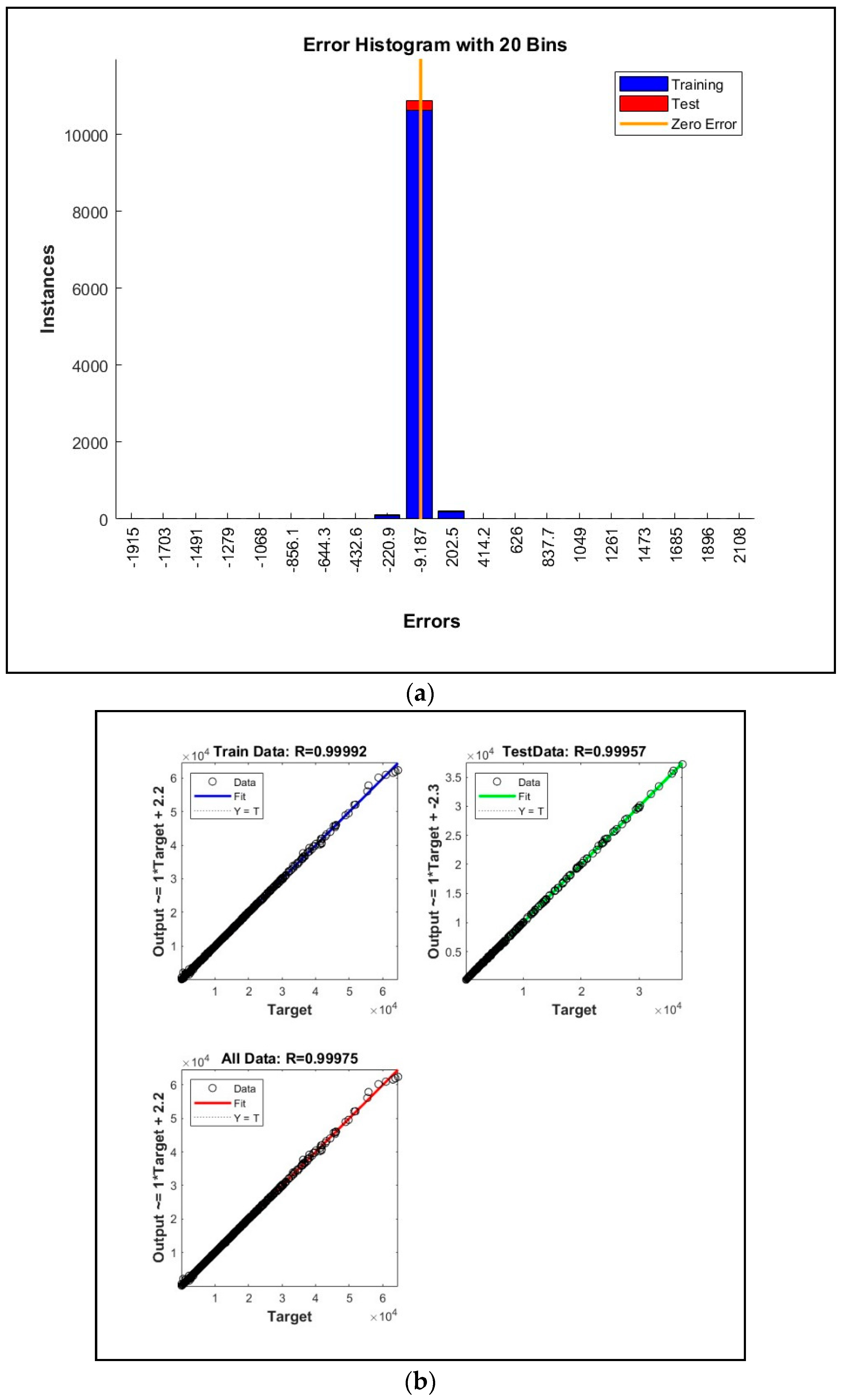