Abstract
This article introduces Signal Tables as a format to exchange data associated with simulations based on dictionaries and multi-dimensional arrays. Typically, simulation results, as well as model parameters, reference signals, table-based input signals, measurement data, look-up tables, etc., can be represented by a Signal Table. Applications can extend the format to add additional data and metadata/attributes, for example, as needed for a credible simulation process. The format follows a logical view based on a few data structures that can be directly mapped to data structures available in programming languages such as Julia, Python, and Matlab. These data structures can be conveniently used for pre- and post-processing in these languages. A Signal Table can be stored on file by mapping the logical view to available textual or binary persistent file formats, for example, JSON, HDF5, BSON, and MessagePack. A subset of a Signal Table can be imported in traditional tables, for example, in Excel, CSV, pandas, or DataFrames.jl, by flattening multi-dimensional arrays and not storing parameters. The format has been developed and evaluated with the Open Source Julia packages SignalTables.jl and Modia.jl.
1. Introduction
In [1] the authors analyzed how to improve the development of credible models based on Modelica Association standards such as the Modelica language [2] (https://github.com/modelica/ModelicaSpecification, accessed on 30 July 2022) or FMI (Functional Mock-up Interface) [3,4,5] (https://fmi-standard.org/downloads/, accessed on 30 July 2022). Their analysis showed that there are various areas where improvements are needed. One of these areas is the exchange of simulation results data between tools, with the overall goal of storing the result of a simulation in a standardized (non-proprietary) format on file, in order that all essential information is available to reproduce simulation runs. Such data should be useable both by post-processing tools and for archiving it, e.g., for traceable quality measures as needed for a credible simulation process. Currently, no satisfactory standardized format of this kind is known; see the analysis in Section 2 (a slightly improved version of Section 4.4 of [1]). There are further requirements that current formats do not support:
- Clocked variables are only defined at clock ticks, and are undefined otherwise.
- In the recently published FMI 3.0 [5], array sizes can change at event points.
- In certain experimental simulators, variables can appear and disappear during a simulation; see for example [6,7].
These requirements mean that variables or variable elements are not defined over all time instants of a simulation. Furthermore, the result of a simulation often undergoes additional processing. As a simple use case, the absolute difference of two variables shall be computed, and one or both variables or variable elements are not defined at all time instants. It would be very helpful if simple standard operations in programming languages, e.g., array subtraction, could be used to express such actions.
2. Overview of Existing Formats
Simulation results are usually stored in a file in binary or ASCII format. This includes reference data as input for a model as well as reference results that a simulation should reproduce within some tolerance. Most simulators have their own proprietary storage format. For example, Simulink (https://www.mathworks.com/help/simulink/, accessed on 30 July 2022) can store simulation data in various ways in the proprietary MAT-file format (https://www.mathworks.com/help/simulink/ug/export-simulation-data-1.html, accessed on 30 July 2022). Simpack (https://www.3ds.com/products-services/simulia/products/simpack/, accessed on 30 July 2022) stores simulation data in its proprietary Simpack Binary Result file format, SBR. Nearly all simulators offer an export of simulation results in CSV format; see the discussion in Section 2.1. When exporting simulation data on file, also other standard serialization formats are in use; see the discussion in Section 3.5.
This section provides a short overview of existing solutions that are typically used or have been proposed for Modelica Association standards to store data from simulation of a Modelica [2] or FMI model [3,4] in a standardized manner. Hereby, compression techniques are utilized that are useful for object-oriented models.
2.1. CSV Format
When results need to be exchanged, such as reference results of the Modelica Standard Library (https://github.com/modelica/ModelicaStandardLibrary, accessed on 30 July 2022) or of an FMI model, they are often stored in CSV format (https://en.wikipedia.org/wiki/Comma-separated_values, accessed on 30 July 2022) thanks to its widespread support in tools. Hereby, a result data set is seen as a table, where every column has a name (optionally with “.” marks to indicate hierarchical structures and “[..]” to mark elements of an array) and represents a time series. The first column contains the monotonically increasing values of the independent variable, usually Time). A discontinuity is indicated by two identical time instants; for an example, see Listing 1.
| Listing 1. Example of a CSV file with a time event at 0.1 s. |
 |
The essential advantage of this format is its simplicity and its widespread support. However, there are numerous drawbacks. In particular, it is not suited for the large data sets needed to archive simulation results. Also, additional data cannot be stored, such as parameters or simulation metadata.
2.2. DSRES Format
The DSRES (Dynamic System RESult) storage format was developed in 1996 for larger result data sets of object-oriented models by the author of this article. It is supported by Dymola (https://www.3ds.com/products-services/catia/products/dymola/, accessed on 30 July 2022), OpenModelica (https://openmodelica.org/doc/OpenModelicaUsersGuide/latest/technical_details.html#the-matv4-result-file-format, accessed on 30 July 2022), Wolfram System Modeler (https://reference.wolfram.com/system-modeler/UserGuide/SimulationCenterSimulationResultFiles.html#92254, accessed on 30 July 2022), and other tools. There are several importing and exporting scripts available, especially for MATLAB and Python (https://github.com/jraedler/DyMat/, https://github.com/kdavies4/ModelicaRes, accessed on 30 July 2022). The DSRES-format consists of a set of matrices that are either stored in MATLAB’s MAT v4 binary format (https://www.mathworks.com/products/matlab.html, accessed on 30 July 2022) or in a textual format. The logical view is as follows:
- The string vector name contains the names of the signals. An index i of this vector characterizes the corresponding signal i. An array variable is flattened into scalar variables. For example, a vector v of length 3 with name "v" is flattened into three signals: name = ["v[1]", "v[2]", "v[3]"].
- The string vector description contains a description text for every signal. The unit of a variable is stored at the end of every description text, e.g., "…[N*m]".
- The integer matrix dataInfo[:,4] contains information on where and how a signal is stored. A signal i is stored:
- in matrix data_j (see next item) with j = dataInfo[i,1];
- in column |k| of matrix data_j with sign(k) as a sign where k=dataInfo[i,2];
- with an interpolation type dataInfo[i,3] (0: linear interpolation);
- with an extrapolation type dataInfo[i,4] (=: undefined outside matrix, 0: keep first/last value outside matrix, 1: linear interpolation through first/last two points outside matrix).
- The core data is stored in the matrices data_j, where every column of a matrix contains the time series of one signal. The first column is the independent variable. Different matrices can have different time axes, that is, a different number of rows. Typically, two data matrices are present: one matrix with two rows that stores the parameters as time series with the first and the last time points, and one matrix with the time-varying signal data, which corresponds to the data stored in CSV file format.
Due to the connector definition, a Modelica model typically has many variables that are identical or have opposite signs. The time series of these signals are stored in a compact way with the DSRES format, as the actual time series of variables that are related by the equations are stored in one column of a data matrix. If all variables of a Modelica model are stored in a result file, the size of the file can often be reduced by a factor of four to five using this technique.
A drawback of this format is that only floating point numbers are defined (integers and Booleans need to be mapped to floating-point numbers, and string values cannot be stored; it would be easy to generalize this format by storing the type of a variable while storing the values of every variable type in a separate data_j matrix; however, this was not done); furthermore, additional attributes and metadata cannot be stored. MATLAB MAT v4 is a very old format that is seldom used today. The DSRES format was not designed (and is not suited) for use inside a program to directly perform convenient post-processing operations on simulation results.
2.3. HDF5-Based Formats
There have been a few attempts to define a standardized time series file format based on HDF5 (https://www.hdfgroup.org/solutions/hdf5/, accessed on 30 July 2022), an open source file format that supports large, complex, and heterogeneous data along with meta-information stored hierarchically in one binary file, in particular, the MTSF format (Modelica Association Time Series File Format) [8] and the SDF format (Scientific Data Format) (https://github.com/ScientificDataFormat, accessed on 30 July 2022). In [8], it was reported that simulation results up to 200 GB could be stored and retrieved in HDF5 format on file. Although, HDF5 appears attractive for scientific data sets, especially simulation result data, it has practical drawbacks: it is complex, there is essentially only one reference implementation in C, and it is not suited for today’s cloud services. For a more detailed discussion, see Section 1 in [9].
2.4. Recon Format
A more modern design is the recon format [9] (https://github.com/xogeny/recon, accessed on 30 July 2022), in which simulation results, additional attributes and other metadata are stored in a network-friendly way in either of two ways. Hereby, the core data is packed with msgpack (https://msgpack.org/, accessed on 30 July 2022) with additional structure on top of it based on the JSON data model (https://www.json.org/json-en.html, accessed on 30 July 2022). In [9], tests were conducted to compare the recon format with the DSRES format. The few tests performed indicate that the recon format needs about less storage, writes data about faster, and reads data about faster than the DSRES format, meaning that the recon format outperforms the DSRES format. The recon format is not designed (and is not suited) for use inside a program to perform convenient post-processing operations on simulation results.
3. Signal Tables
A Signal Table is basically a standard table in which the table columns can be multi-dimensional arrays and additional attributes can be stored with every array and with the table. In this section, a Signal Table is defined with a combination of ordered dictionaries (ordered key/value pairs), multi-dimensional arrays, and scalars (string, floating-point, integer, Boolean, etc., variables). This view can be directly mapped to data structures available in programming languages such as Julia [10] (https://julialang.org/, accessed on 30 July 2022), Python (https://www.python.org/, accessed on 30 July 2022), and MATLAB (https://www.mathworks.com/products/matlab.html, accessed on 30 July 2022). Below, the notation is used by which a variable means the variable of the underlying model from which a Signal Table is produced, while a signal of a Signal Table holds all the values of this model variable produced from one or more simulation runs, as well as all attributes associated with the model variable (such as its units).
First, a simple example of a Signal Table is provided in Section 3.1; then, the formal definition of a Signal Table is provided in Section 3.2.
3.1. Simple Example of a Signal Table
The Julia code in Listing 2 shows how the Julia language can be used to define a simple Signal Table consisting of the signal "time" (from the model variable ) and the signal "motor.angle" (from the model variable ).
| Listing 2. Simple Signal Table. |
 |
Here, SignalTable(..) is a constructor of a Julia dictionary in which key => value defines a new key and its value. The keys are defined with strings (e.g., "motor.angle"). Var(..) is a constructor of a Julia dictionary that holds the values and all attributes associated with a signal. As the keys of Var dictionaries are not hierarchical, it is more convenient for these dictionaries to use Julia symbol keys instead of string keys, as Julia has special support for them. When exporting to a file, string keys are used. For this reason, the value associated with the key "motor.angle" is defined as above and not as Var("values" => sin.(t), "unit" => "rad", …). The command showInfo(sigTable1) generates the output shown in Listing 3.
| Listing 3. Information about simple Signal Table. |
 |
As can be seen, the "time" and "motor.angle" values vectors have a size of 101 (the key "values" of the signal "time" has the value [0.0, 0.1, 0.2, ..]; the key "values" of the signal "motor.angle" has the value [0.0, 0.99.., 0.19.., …]). The size of an array, and thus the sizes of all its dimensions, is provided as a vector of integers. The element type of these vectors, abbreviated as eltype, is Float64. The plot(..) call generates Figure 1.
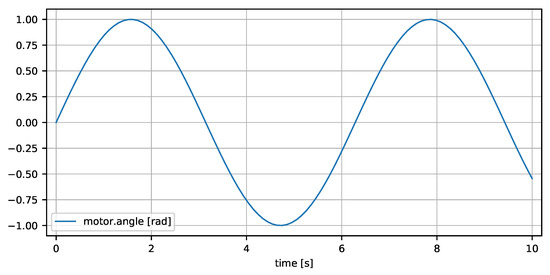
Figure 1.
Plot of simple Signal Table of Listing 2.
Below, the notation motor.angle[i] is the value of the variable at time[i], and is stored in the key "values". For example, motor.angle[3] = sin(time[3]) = sin(0.2) = 0.198… is the value of the model variable at time[3] = 0.2. Here, it is assumed that the first value of a vector has an index of one (as in Julia and MATLAB) and not zero (as in Python).
3.2. Formal Definition of a Signal Table
A Signal Table is an ordered dictionary of signals with string keys that hold the hierarchical names of the signals (for example, key = "a.b.c") and with values that are either Var, Par, or Map dictionaries:
- A Var (=abbreviation for Variable) dictionary has a required key "values" with an associated value that is a multi-dimensional array of any element type and has one of the following formats (where is variable k and v_k is the associated value of the key "values"):
- −
- v_k is a vector within the i-th Var that has attribute "independent" = true:v_k[:] are the values of independent variable .
- −
- v_k is a vector with only one independent variable defined:v_k[i] is the value of scalar variable at independent variable .
- −
- v_k is a matrix with only one independent variable defined:v_k[i,j] is the value of at independent variable .
- −
- v_k is an array with two or more dimensions:v_k[i1,i2,…in,j1,j2,…jm] is the value ofat independent variables .
- A Par (=abbreviation for Parameter) dictionary has a required key "value" representing a parameter of any type and does not depend on the independent variables.
- A Map dictionary has no required keys, and collects attributes/metadata that are associated with a Signal Table or a Var or Par dictionary.
In all dictionary types, optional attributes can be stored with key/value pairs, for example, the keys "independent", "unit", "info", "start", variability", and "alias". The predefined attributes are defined in Appendix A. Applications can add additional attributes.
The Var, Par and Map dictionaries have been derived from the concepts developed by Hilding Elmqvist for the modeling language Modia [11]. In particular, every Modia Var, Par, and Map dictionary is a subset of the corresponding Signal Table dictionary (with exception of unit handling). Differences include that a Var dictionary in Modia does not have a "values" key and that units are stored via a separate "unit" key in a Signal Table, whereas units are associated directly with values in Modia via the Julia package Unitful.jl (https://github.com/PainterQubits/Unitful.jl, accessed on 30 July 2022).
In order to cope with undefined (missing) values, a value or element of an array can have a value that is called missing, which is the notation used by the Julia language. High-level programming languages support this concept in various forms; additional details are provided in Section 3.4. The basic goal is that operations of any type are supported for missing values. For example, the result of two operands is missing if one or both have a value of missing, e.g., is or is . Missing values are useful for supporting undefined values in any kind of operations in a convenient way.
If a Signal Table stores all variables with a start attribute, all parameters, a unique identification of the model, the attributes for the experiment setup, a tool identification (name,version), information to build the executable version of the model (e.g., name, version, options of compiler, make file, …), and the operating system (name,version), it is possible to reproduce the simulation run by
- using the tool and build information on the respective operating system,
- instantiating the corresponding model,
- initializing variables with the start attributes,
- using the values of the parameters from value,
- simulating with the attributes from Map experiment (see Table A3),
- setting absolute and relative tolerances with the help of the nominal, unbounded, tolerance attributes (for details, see FMI 3.0 [5]).
When used in this way, Signal Tables are one piece in a credible simulation process, because every simulation result contains enough information to reproduce it.
3.3. Examples
In this section, various examples are used to demonstrate the ways in which Signal Tables can be utilized. All of these examples have been defined and the results produced using the open source Julia package SignalTables.jl (https://github.com/ModiaSim/SignalTables.jl, accessed on 30 July 2022) based on the Julia programming language. Package SignalTables.jl provides about 35 functions operating on Signal Tables; see section Overview of Functions (https://modiasim.github.io/SignalTables.jl/stable/Functions/OverviewOfFunctions.html, accessed on 30 July 2022). Several of them are used below, accompanied by a short explanation.
In principle, these examples can be carried out in a similar way in other high-level programming languages such as Python and MATLAB.
3.3.1. Various Signal Table Types
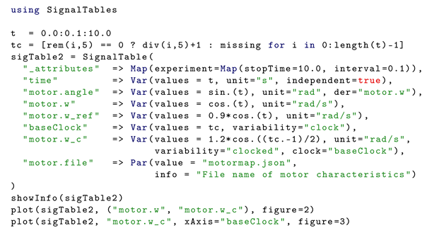
In the Signal Table of Listing 4, various different types of signals are defined.
Here, "_attributes" is a signal with attributes/metadata defined for the Signal Table. tc is an integer vector [1,missing,missing,missing,missing,2,missing,…] which holds the tick numbers of a clock (or is missing if the clock is not active). This vector is stored as "baseClock" with variability="clock" in the Signal Table. The signal "motor.w_c" is a Float64 signal that has a value at every clock tick. The attribute der="motor.w" of the signal "motor.angle" defines "motor.w" as being the derivative of "motor.angle" with respect to the independent variable "time". The signal "motor.file" is a string parameter. The command showInfo(sigTable2) generates the output shown in Listing 5.
| Listing 4. Signal Table with various types. |
 |
| Listing 5. Information about Signal Table with various types. |
 |
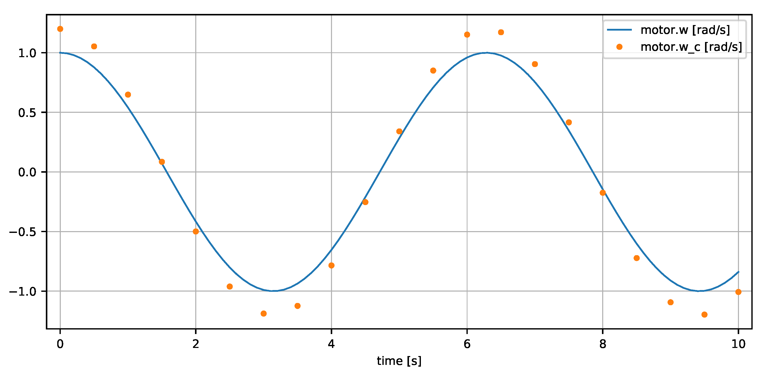
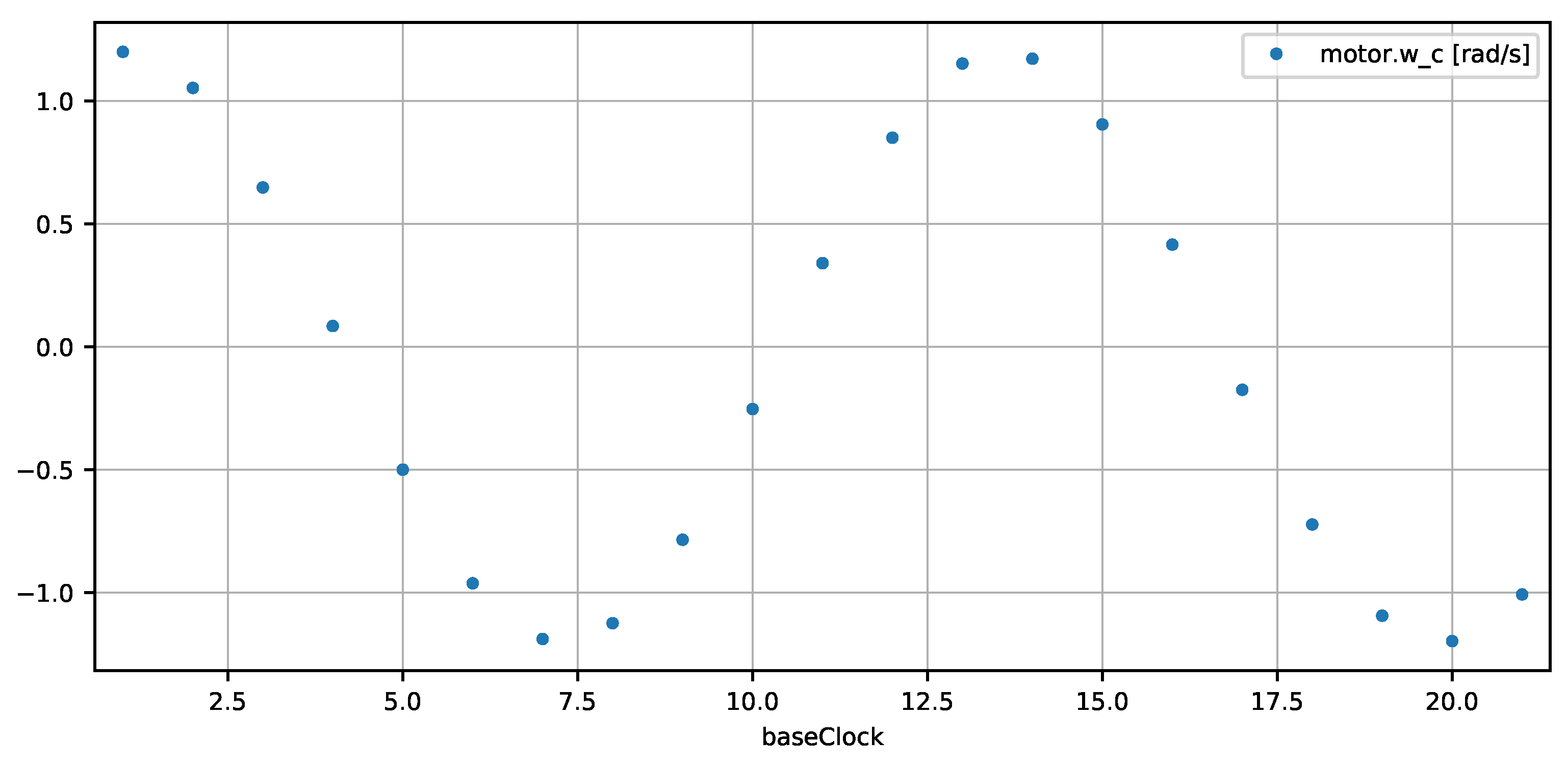
If an array has missing values, its Julia element type is Union{Missing,XXX}, meaning that this type includes all instances of any of its argument types as objects. The plot(..) commands generate Figure 2.
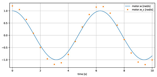
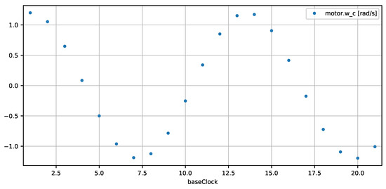
Figure 2.
Plot of Signal Table with various types.
In the first plot, the continuous signal "motor.w" and the clocked signal "motor.w_c" are shown. As missing values are ignored in a plot, the missing values of "motor.w_c" are not shown. The second plot(..) call has the signal "baseClock" as the x-axis, thus, an integer vector with the numbers 1,2,…,21 of the clock ticks.
Because signal values are arrays, array operations can be conveniently used for post-processing. An example is shown in Listing 6.
| Listing 6. Post-processing of Signal Table with various types. |
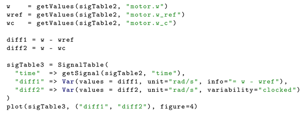 |
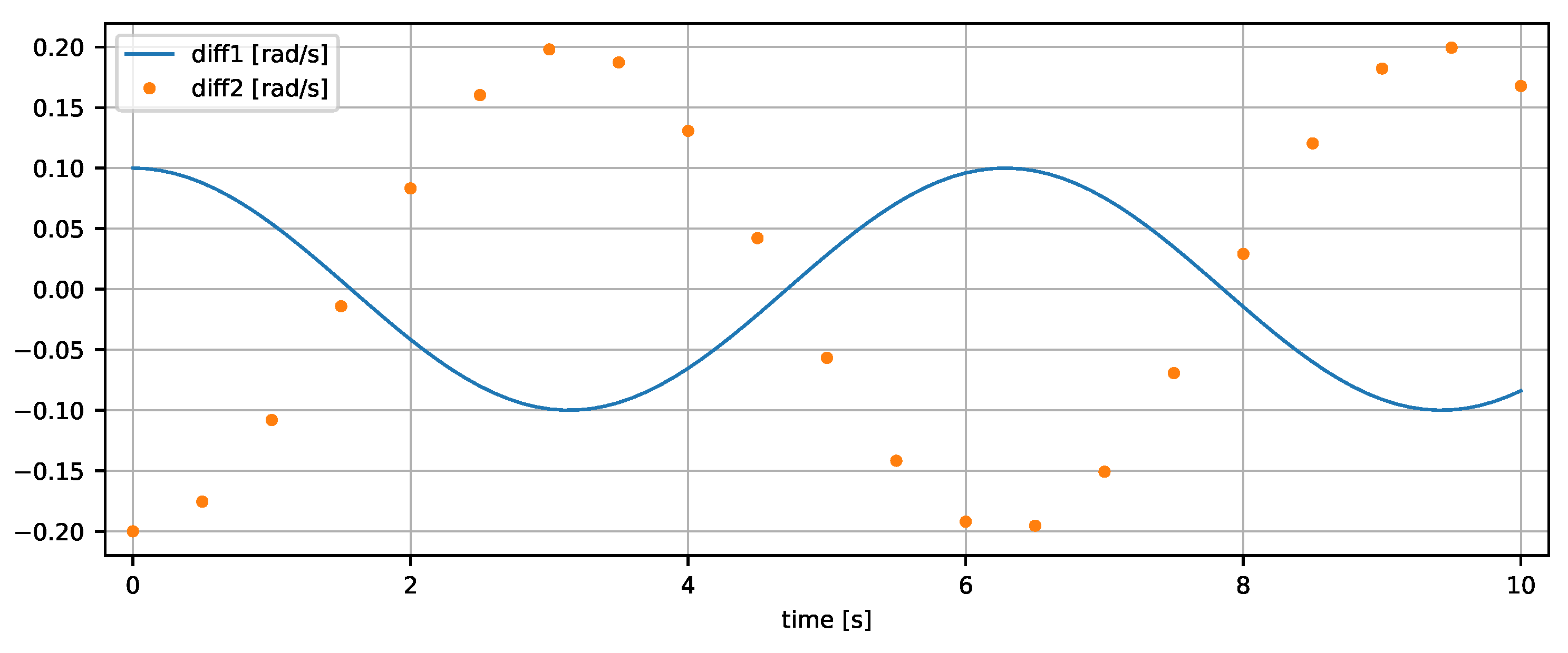
In this example, the differences of the continuous signals "motor.w" and "motor.w_ref" as well as the differences of the continuous signal "motor.w" and the clocked signal "motor.w_c" (which has missing values) are computed and plotted. The result is shown in Figure 3.
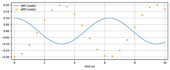
Figure 3.
Plot of post-processed signals of Signal Table with various types.
3.3.2. Transient Simulation
To demonstrate various aspects of simulation result handling, the very simple first order system defined in Equation (1) is simulated below in various ways.
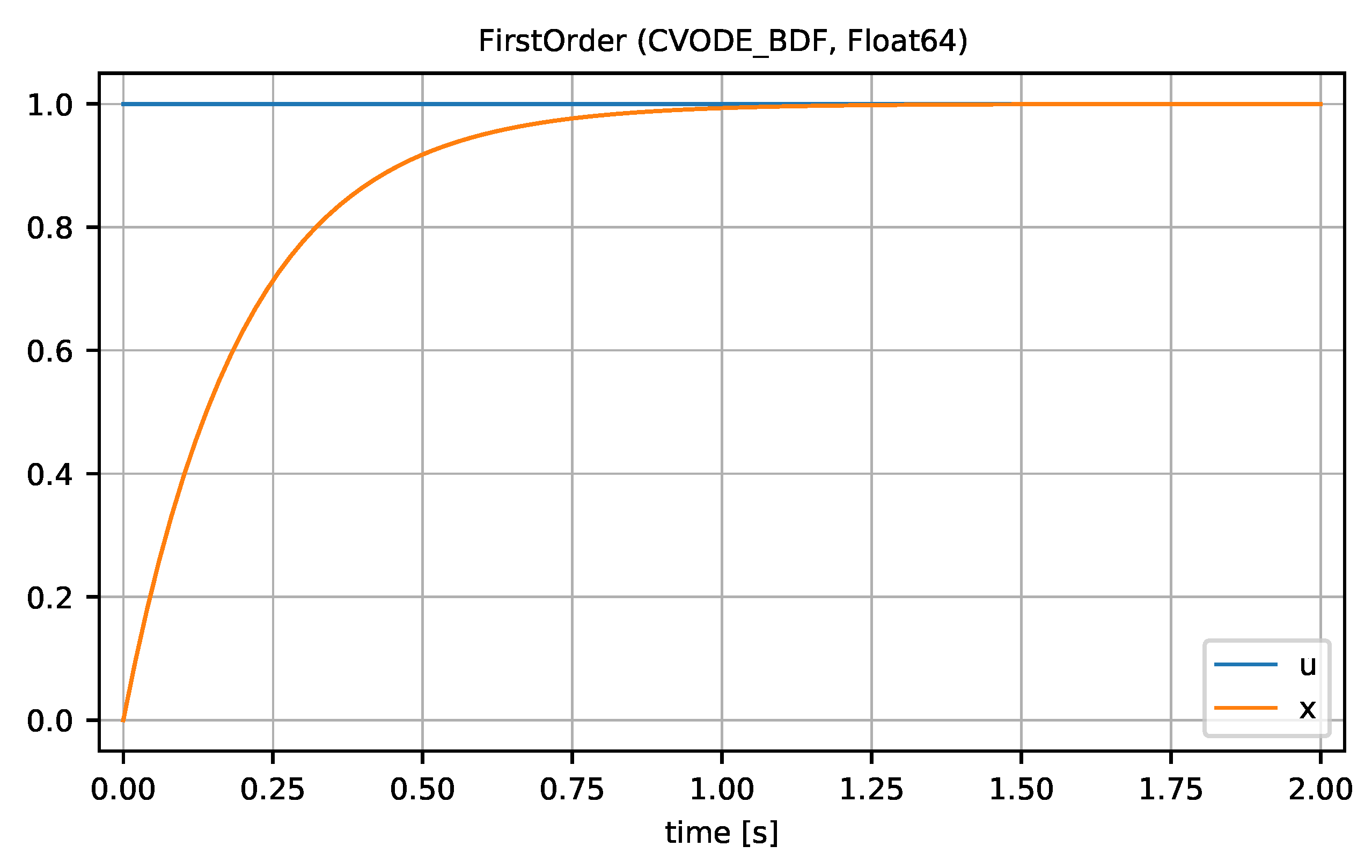
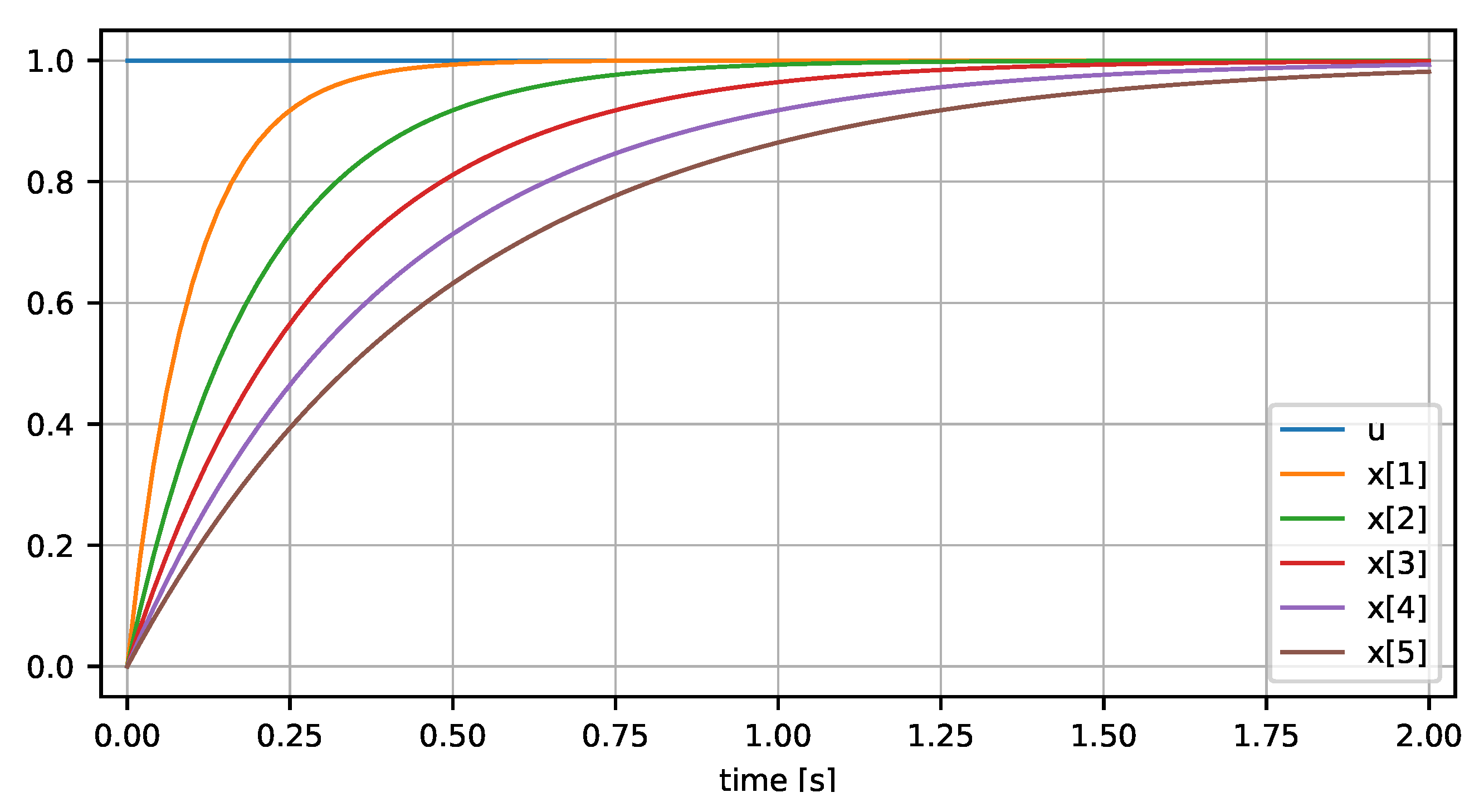
Here, is a state with the initial value , is an input, and are parameters. Modia [11] is used to define and simulate this system with , , , and . Simulation results are shown as Signal Table in Listing 7 and a plot of "u" and "x" is shown in Figure 4.
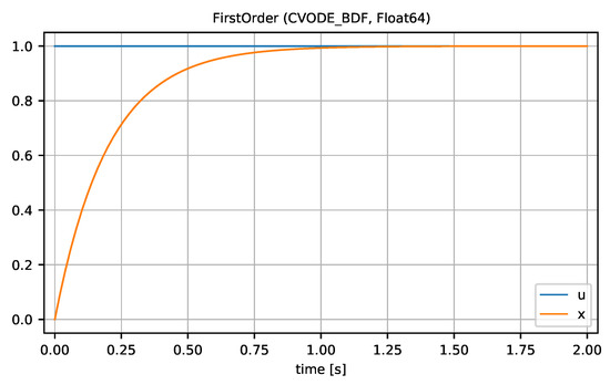
Figure 4.
Simulation result of one simulation with , , , and .
| Listing 7. Signal Table of one simulation of model firstOrder. |
 |
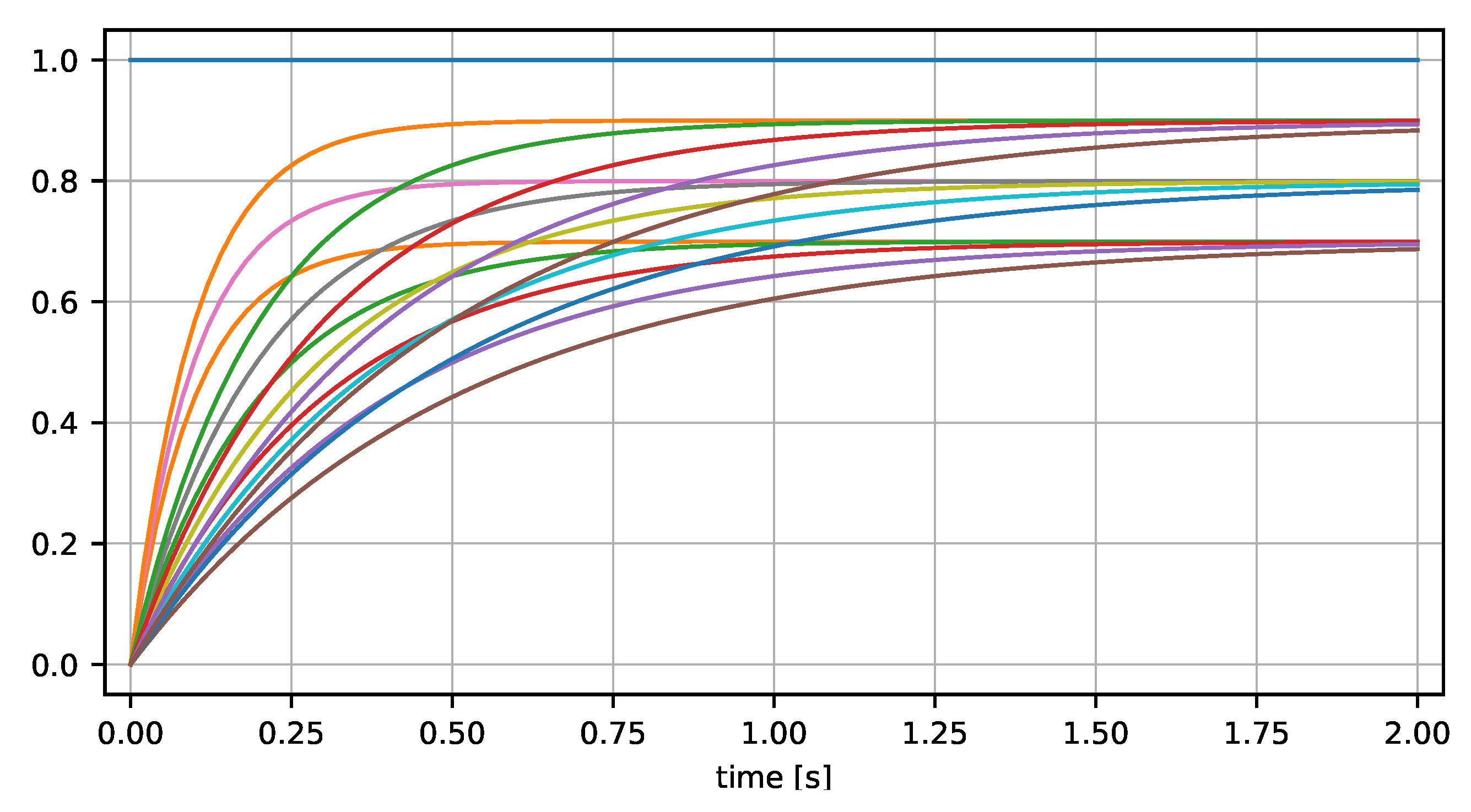
Simulations can be carried out for various values of T and collected together in one Signal Table; see Listing 8.
| Listing 8. Parameter variation of model firstOrder resulting in one Signal Table based on five simulations where the first independent variable is "time" and the second independent variable is "T" with values = 0.1, 0.2, 0.3, 0.4, 0.5. |
 |
Because "T" is varied, this signal is no longer a parameter and is instead an independent variable defined as a vector with five elements: . The other variables have a size of [101,5] instead of [101], as they are functions of two independent variables ("time", "T"). Note that the complete information of the parameter variation is stored in this Signal Table, and therefore the parameter variation can be reproduced, for example, as needed for a credible simulation process. A plot of "u" and "x" is shown in Figure 5.
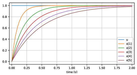
Figure 5.
Parameter variation of model firstOrder with , , , and .
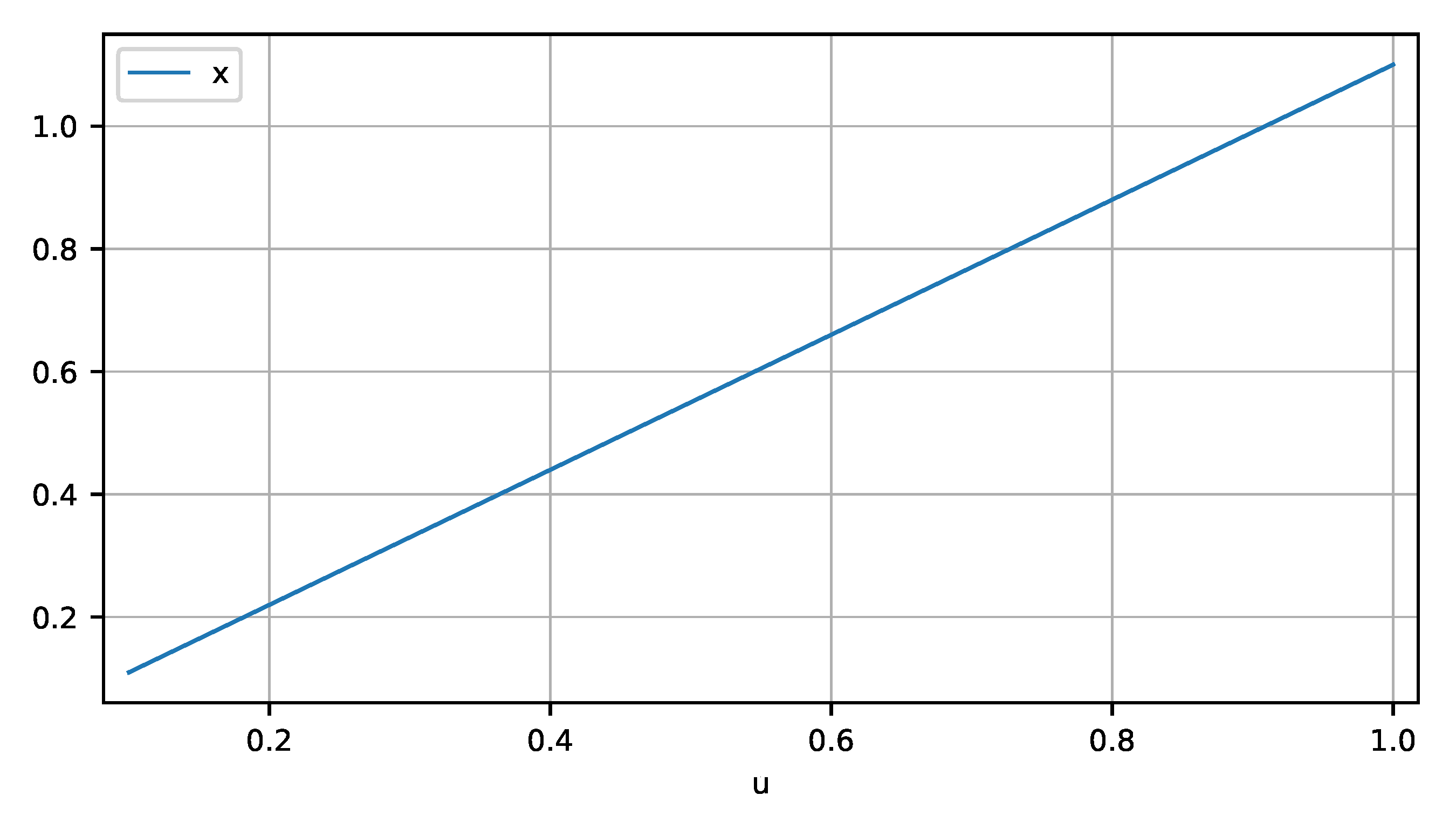
Additionally, two or more parameters can be varied. This is demonstrated by additionally varying k with the values , leading to a Signal Table with three independent variables; see Listing 9.
| Listing 9. Parameter variation of model firstOrder resulting in one Signal Table based on 5 × 3 simulations in which the first independent variable is "time", the second independent variable is "T" with values = 0.1, 0.2, 0.3, 0.4, 0.5, and the third independent variable is "k" with values = 0.7, 0.8, 0.9. |
 |
Because the result of the complete parameter variation simulations is stored in one Signal Table, post-processing is again convenient, as array operations can be directly applied on the signal variables, which in this case are three-dimensional arrays. A plot of "u" and "x" is shown in Figure 6. The legend is no longer displayed in the plot, as there are too many curves, although the legend remains available via the plot toolbar.

Figure 6.
Parameter variation of model firstOrder with , , , and .
Monte Carlo simulation, worst case optimization, multi-criteria optimization, etc., could be handled in a similar way as shown above for parameter variations. However, this would not be practical because many more independent variables are present and not all combinations of the independent variables are evaluated. Such applications are treated by enumerating the respective simulations with an integer and having this integer as a second independent variable. For example, the parameter variation with T and k can be performed as shown in Listing 10.
| Listing 10. Parameter variation of model firstOrder resulting in one Signal Table based on 15 simulations in which the first independent variable is "time" and the second independent variable is "run" with values = 1, 2, …, 15. |
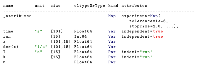 |
The difference is that there is a new independent variable, "run" (shorthand for number of simulation run), with the values 1, 2, …, 15, that enumerates all evaluated variations of T and k. All time-varying variables are a function of "time" and "run". For example, "x" has size [101,15] instead of [101,5,3] as in Listing 9. Furthermore, T and k are no longer Var signals, and instead are stored as Par signals "T", "k" with size [15], and their relationships to "run" are marked with the key index1 = "run" (e.g., k[i] is the value of k at run[i]). A plot of "x" results again in Figure 6 (only the legends are different, although this is not shown in the figure).
For Monte Carlo Simulation, worst case optimization, multi-criteria optimization, etc., additional data need to be defined. For example, assume that a Monte Carlo Simulation is performed in which T, k, and the start value of x are randomly selected. Assume that k is described by a uniform distribution. Then, this information can be stored together with k as shown in Listing 11.
| Listing 11. Signal Table of a Monte Carlo Simulation run where the parameter k is defined with a Uniform distribution in the range 0.7 . . . 1.1. |
 |
Additional details on defining uncertainty descriptions and other data for credible model descriptions are provided in the companion paper [12].
3.3.3. Steady-State Simulation
In a steady-state simulation, either the derivatives are set to zero and a (usually nonlinear) equation system is solved for the unknowns, or one simulation is carried out for a long time until there are no more variations in the states. In both cases, the result of one steady-state simulation is one value for every variable. With , the first order model is transformed to the (trivial) steady-state model of Equation (2):
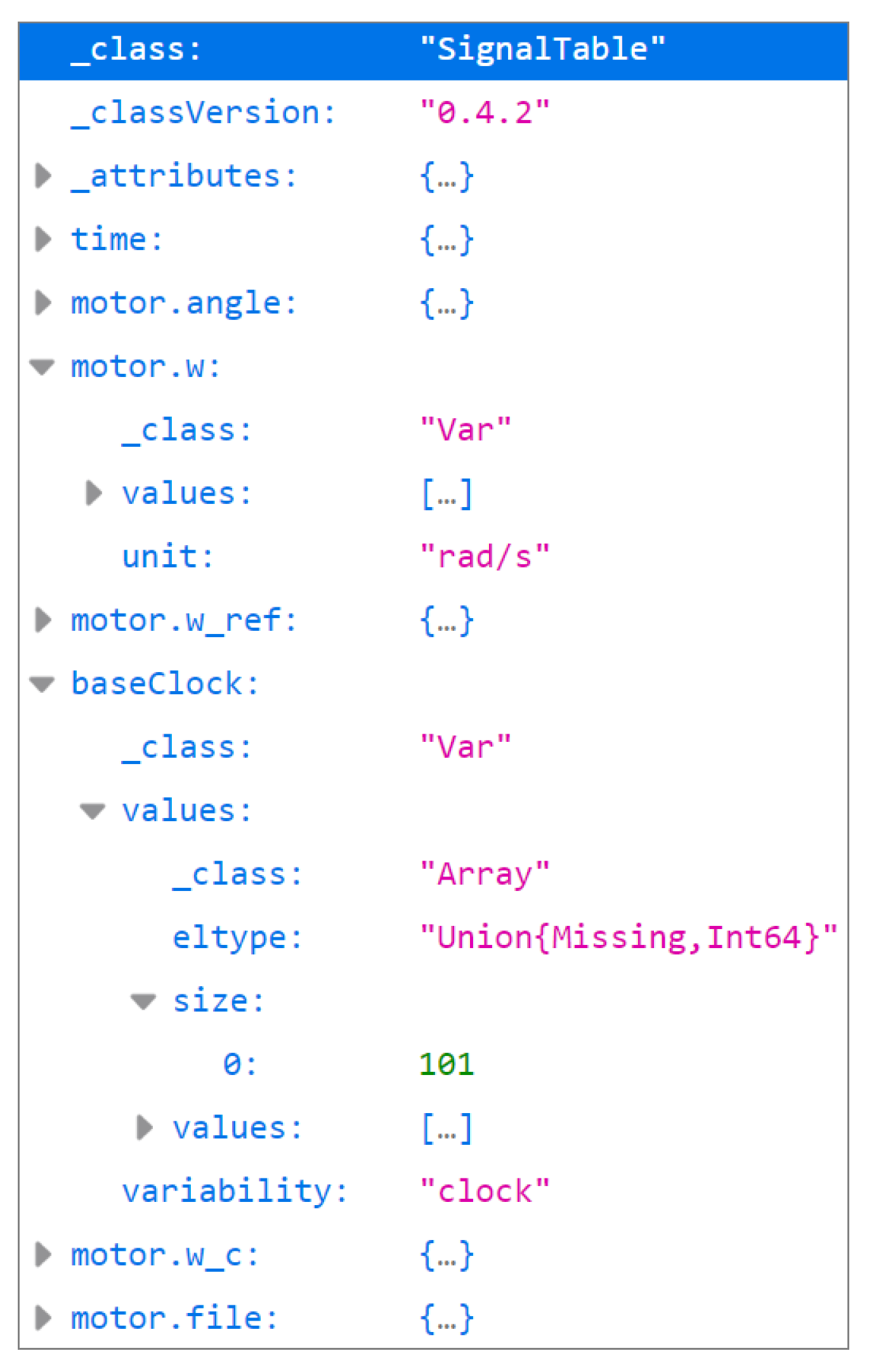
By varying u with values 0.1:0.1:1.0, again, one Signal Table is constructed; see Listing 12.
| Listing 12. Steady-state simulations of model firstOrder resulting in one Signal Table. |
 |
In a steady-state simulation, it is sometimes useful to add a signal "stopTime" containing the time instants when the underlying transient simulation reached its steady-state condition. A plot of "x" over "u" is shown in Figure 7.
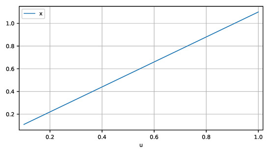
Figure 7.
Steady-state simulations of model firstOrder with and .
3.4. Missing Values
This section gives a brief overview of how missing values are handled in various programming languages and file formats:
- In the Julia language, a missing value of any type is represented by the value missing. The properties of this design (no efficiency degradation, small memory overhead) are discussed in a blog posting (https://julialang.org/blog/2018/06/missing/, accessed on 30 July 2022).
- In the R programming language (https://www.r-project.org/, accessed on 30 July 2022), a missing value is represented by the value NA (https://rlang.r-lib.org/reference/missing.html, accessed on 30 July 2022), which is converted to a type-specific missing value.
- In Python, there is no dedicated missing value; instead, NaN is used for floating-point types and None is used for Python objects (https://jakevdp.github.io/PythonDataScienceHandbook/03.04-missing-values.html, accessed on 30 July 2022). Certain packages, such as pandas, have special support to make this more convenient.
- In MATLAB, a missing value is supported for certain data types and is represented by the value missing, which is converted to a type-specific value (https://www.mathworks.com/help/matlab/data_analysis/missing-data-in-matlab.html, accessed on 30 July 2022).
- In JSON, a missing value of any type is represented by the value null.
When Signal Table data are passed to a C or C++ function, for example, when calling a plot function, these languages have no concept of missing values. Furthermore, line plot functions usually do not have support for three-dimensional or higher-dimensional arrays, and only support a limited set of types (for example, Bool types are often not supported). In order to cope with these issues, package SignalTables.jl provides a function getFlattenedSignal(signalTable,name) (https://modiasim.github.io/SignalTables.jl/stable/Functions/SignalTables.html#SignalTables.getFlattenedSignal, accessed on 30 July 2022) that returns a copy of a signal where the value or values are potentially flattened into a matrix and/or potentially transformed to Float64 and missing values transformed to NaN; the transformed "values" or "value" are stored in the new key "flattenedValues" and the description is stored in the new key "legend".
For example, a Boolean signal with values=[true, missing, missing, false] receives a new key flattenedValues=[1.0, NaN, NaN, 0.0]. An array signal "myarray" with a size of [100,5,3] receives a new key flattenedValues with a matrix of size [100,15] and a new key
legend = ["myarray[1,1]", "myarray[2,1]", …, "myarray[5,3]"] that provides a meaningful legend for every column of this matrix. When a Signal Table is flattened with getFlattenedSignal, it can be imported in standard table formats such as Excel (https://en.wikipedia.org/wiki/Microsoft_Excel, accessed on 30 July 2022), CSV, pandas (https://pandas.pydata.org/, accessed on 30 July 2022), or DataFrames.jl (https://github.com/JuliaData/DataFrames.jl, accessed on 30 July 2022).
3.5. Signal Tables on File
An essential property of a Signal Table is that it can be stored on file or transported via a network protocol. Potentially, every standardized serialization format can be used for this purpose. Signal Tables are primarily designed for the widespread textual JSON format (https://www.json.org/json-en.html, accessed on 30 July 2022), and can in principle be transformed to any JSON-compatible binary serialization format (such as UPJSON, BSON, MessagePack). A recent comparison of serialization formats is provided in [13]. Furthermore, it is possible to store a Signal Table in HDF5 format (https://www.hdfgroup.org/solutions/hdf5/, accessed on 30 July 2022); see below. All these formats encode data when writing the data to file and decode data when reading the data from file.
Another approach is available via Apache Arrow (https://arrow.apache.org/, accessed on 30 July 2022) and Apache Parquet (https://parquet.apache.org/, accessed on 30 July 2022), in which data is used in a buffered way and communicated without encoding/decoding in order to take modern hardware acceleration into account. For certain large applications, a huge increase in speed is reported (https://voltrondata.com/news/arrow-columnar-analytics/, accessed on 30 July 2022). TileDB (https://github.com/TileDB-Inc/TileDB, accessed on 30 July 2022) builds on top of Apache Arrow for fast storage and accessing of large, dense, and sparse multi-dimensional arrays.
In the following examples, first evaluations of storing Signal Tables via the JSON format are shown. It is outside the scope of this article to perform a detailed analysis of performance when using the JSON format along with evaluation of other options. Tests with the conceptually similar recon format [9] have shown that better performance can be achieved, as with the DSRES format, if the data are compressed appropriately. The evaluation below uses the pure JSON format without compression.
When storing a Signal Table in JSON format, additional metadata are stored and transformations take place for types that cannot be directly represented in JSON to allow reading from such a file to completely restore the original data:
- A dictionary of type SignalTable, Var, Par, Map is stored as a JSON object with an additional element "_class":"<kind>", for example, "_class":"Var".
- An array with more than one dimension is stored as a JSON object with additional information. For example, a Float32 matrix with 4 rows and 2 columns and with values = [11 12; 21 22; 31 32; 41, 42] is stored as a JSON object as shown in Listing 13. Note, the elements of the matrix are stored in a vector in column-major ordering.
Listing 13. JSON object of a Float32 matrix with values = [11 12; 21 22; 31 32; 41, 42]. 
- The "values" and "value" elements of a signal are not written on file if the key "alias" is present. In Julia, the "values" and "value" data of alias signals are present only once and are referenced from corresponding alias signals. When writing to file, the parent alias "values" and "value" data is written on file, while the data of the child alias signals (identified by the "alias" key) are not stored on file. The compression is thus somewhat less than with the DSRES format sketched in Section 2.2 as negative alias signals are not specially handled. In object-oriented modeling, trivial equations of the form often occur. In the DSRES format, the data of one of these variables is stored. With a Signal Table, the data of two of these variables is stored (). This is similar to FMI 3.0 [5], in which negative alias variables are not supported in order to simplify the FMI description (in FMI 1 and FMI 2 [4], negative alias variables are supported).
As an example, sigTable2 from Listing 4 is stored on file "sigTable2.json" with the commands of Listing 14.
| Listing 14. Commands to store sigTable2 from Listing 4 in JSON format on file. |
 |
Several web browsers have special support for conveniently showing JSON files. For example, the result when inspecting the file "sigTable2.json" with Firefox (https://www.mozilla.org/en-US/firefox/, accessed on 30 July 2022) is shown in Figure 8. Inspecting such a file is therefore easy and convenient without additional tool support.
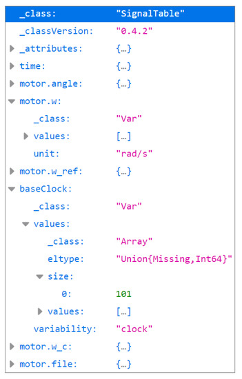
Figure 8.
View of the file sigTable2.json in Firefox. The hierarchy of the JSON objects can be interactively expanded or folded.
Julia has various packages that can be used to store data on file. In particular, the package JLD.jl (https://github.com/JuliaIO/JLD.jl, accessed on 30 July 2022) allows lossless storage of any Julia object in HDF5 format by automatically adding attributes and naming conventions to preserve type information for each object. A Signal Table can be stored with this package with the commands of Listing 15.
| Listing 15. Commands to store sigTable2 from Listing 4 in HDF5 format on file. |
 |
4. Conclusions and Outlook
In this paper, a new format has been proposed for exchanging data associated with simulations based on dictionaries and multi-dimensional arrays. One design goal of this format is that simulation runs become reproducible; that is, all information necessary to redo a run or related runs can be stored. This is one important building block for a credible simulation process. Furthermore, the simple format allows for very convenient post-processing with standard array operations available in high-level languages such as Julia, Python, and MATLAB.
In [9], two formats of the recon file format were proposed, namely, the “Wall” format for writing data as a series of “bricks” in the order that data appear during simulation, and the “Meld” format for writing data in rearranged form such that individual signals can be easily extracted. The “Signal Table” format is similar in spirit to the “Meld” format, and has the same advantages [9]: As simulation moves to cloud based systems, it will be come increasingly cumbersome to move entire files back and forth between the cloud and the desktop/browser. Having a format that supports "pulling" just the information that is required on demand facilitates utilizing cloud/remote storage solutions which will lead to more responsive interfaces and better data management practices and capacity. The meld format is designed for this use case.
There are various possibilities for improvements to the Signal Table format. In particular, a compressed format could be defined such that missing values are not stored, only non-missing values. For example, the values of clocked signals could be stored in separate vectors without missing values together with the information about the underlying clock. If variables are only defined in various phases of a simulation (and are otherwise missing), then only these phases can be stored. This approach is essentially used internally in Modia [11]; although it makes little sense to expose such a complex internal data structure to the user. The high-level view should still be the logical view presented in this article. This is similar to the handling of sparse matrices, for which the user can conveniently perform efficient array operations despite the complexity of their internal data structures.
Currently, Signal Tables can be stored on file in JSON or HDF5 format. It should be possible to reduce the file size of the network-friendly JSON format using compression techniques from recon, e.g., by compressing the values with the msgpack format. An evaluation is needed with respect to the file size and read/write time of large simulation data of the various ways in which a Signal Table can be stored on file. The results should be compared with current simulation result file formats, especially the DSRES and CSV formats.
To enable widespread use, the Signal Table format needs to be supported by many simulation tools. In this respect, it is important to begin discussion with interested tool vendors. Fine-tuning iteration might be needed to more precisely define all pieces of the format as well as to eventually adapt corner cases and define further standardized attributes.
Funding
This work was organized within the European ITEA3 Call6 project UPSIM (https://itea3.org/project/upsim.html, accessed on 30 July 2022)—Unleash Potentials in Simulation, grant number 19006. This work was partially funded by the German Federal Ministry of Education and Research (BMBF), grant number 01IS20072H.
Data Availability Statement
The Julia package SignalTables is publicly available from https://github.com/ModiaSim/SignalTables.jl (accessed on 30 July 2022) under the MIT open source license.
Acknowledgments
I would like to thank Andreas Pfeiffer, Leo Gall, Hilding Elmqvist, and Jakub Tobolář for their constructive improvement proposals.
Conflicts of Interest
The author declares no conflict of interest.
Appendix A. Predefined Attributes of a Signal Table
In the following Table A1, Table A2 and Table A3, the predefined attributes of the respective dictionary types are summarized. Most keys in these tables are identical (or similar) to the attributes defined in Sections 4.8 and 18.4.1 in the Modelica Specification 3.5 [2] and the attributes defined in Sections 2.4.6 and 2.4.7 in the Functional Mock-up Interface Specification 3.0 [5], with the exception that the Modelica/FMI attribute description is called info.

Table A1.
Predefined attributes for Var dictionaries. Either "values" or "alias" must be present. During the construction of a signal table, all Var with the attribute "alias" are automatically processed and obtain a "values" key that references the "values" key of the alias variable. As a result, "values" is present for all Var dictionaries after the construction of a Signal Table. All other keys are optional.
| Key | Value | Value |
|---|---|---|
| Type | Description | |
| "info" | String | Short description of signal. |
| "independent" | Bool | = true, if independent variable (i-th independent variable is i-th Var in signal
table with "independent" = true). If not present, "independent" = false. |
| "values" | Any | See Section 3.2. Elements have units defined with attribute "unit". |
| "alias" | String | Key of alias signal (see caption). |
| "unit" | String | Unit of all signal elements, e.g., "kg*m*s^2". |
| String Array | unit is unit of variable element . | |
| "displayUnit" | String | Display "values" with respect to "displayUnit". using "displayUnit" for all signal elements. |
| String Array | displayUnit is display unit of variable element . | |
| "start" | Any | Initial value of variable. |
| "fixed" | Bool | = true, if the variable value is "start" after initialization. = false, if the variable value is "start" before initialization (default = false). |
| "nominal" | Float64 | Nominal value of all variable elements. |
| "unbounded" | Bool | = true indicates that during time integration, the variable gets values much larger than its nominal value. Typically, relative tolerance is set to zero to increase numerical stability, see FMI 3.0 [5] (default = "false"). For example, the rotation angle of a vehicle shaft would be typically defined with "unbounded=true". |
| "variability" | String | = "continuous", "clocked", "clock", "discrete" or "tunable". "tunable" is similar to "discrete" but characterizes a parameter that is changed/tuned during simulation (default = "continuous"). |
| "state" | Bool | = true, if signal is a (continuous, clocked or discrete) state (default = false). |
| "der" | String | Key of variable that is the derivative of the variable with respect to the first independent variable. |
| "previous" | String | Key of variable that is the previous value of the variable at the current clock tick. ("variability" must be "clocked" or "clock"). |
| "clock" | String | Key of clock associated with variable (values is only defined at clock ticks and otherwise is missing). |
| "interpolation" | String | Interpolation of signal points (= "linear" or "none"). If not provided, "interpolation" is deduced from "variability" and otherwise it is "linear". |
| "extrapolation" | String | Extrapolation outside the values of the independent signal (= "none", "HoldLastPoint", "LastTwoPoints"; default = "none"). |
In object-oriented modeling, trivial equations of the form , , often occur. For a Signal Table, the data of two of these variables is typically stored, for example, , and variables are defined as aliases of , and variable is defined as an alias of variable . This is similar to FMI 3.0 [5], in which alias variables are defined, as opposed to the negative alias variables used in FMI 1 and FMI 2 [4], simplifying the FMI description and its usage.
Units are defined as strings. There is no accepted standard for a string representation of units. In a Signal Table, units are stored in the format of the generation tool. When using the Julia package SignalTables, units are stored according to the string representation of the Julia package Unitful, for example, unit="kg*m*s^2". Unitful has a precise and coherent type system of units, and all operations can be carried out with units; for example, 0.5u"m" + 20u"cm" results in 0.7u"m". When using a Modelica tool, units are stored according to the Modelica unit definition, for example, unit = "kg.m.s-2". The used unit format is defined in a Signal Table with the attribute "unitFormat" in the Map "attributes"; see Table A3. The string representation of units in Unitful is similar to the string representation of units of the Modelica Specification 3.5 [2] in Section 19, with the following essential differences:
- Multiplication is characterized by "*" in Unitful and by "." in Modelica.
- Exponentiation is characterized by "^" in Unitful and without a symbol in Modelica.
- Degree is characterized by "°" in Unitful and by "deg" in Modelica.
For example, "kg*m*s^-2" in Unitful is represented in Modelica as "kg.m.s-2". If necessary, it is therefore straightforward to convert between string representations in Modelica and in Julia/Unitful.

Table A2.
Predefined attributes for Par dictionaries. Either "value" or "alias" must be present. During the construction of a signal table, all Par with the attribute "alias" are automatically processed and obtain a "value" key that references the "value" key of the alias variable. As a result, "value" is present for all Par dictionaries after the construction of a Signal Table. All other keys are optional.
| Key | Value | Value |
|---|---|---|
| Type | Description | |
| "info" | String | Short description of signal. |
| "value" | Any | Value of any type (does not depend on independent signals). |
| "alias" | String | Key of alias signal (see caption). |
| "unit" | String | Unit of all signal elements, e.g., "kg*m*s^2". |
| String Array | unit[j1,j2,…] is unit of variable element . | |
| "displayUnit" | String | Display "value" with respect to "displayUnit". using "displayUnit" for all signal elements. |
| String Array | displayUnit[j1,j2,…] is display unit of variable element . | |
| "index1" | String | See example of Listing 10. |

Table A3.
Predefined attributes for Map dictionaries. A Signal Table can have an optional key "attributes" that is a Map with the optional attributes below.
Table A3.
Predefined attributes for Map dictionaries. A Signal Table can have an optional key "attributes" that is a Map with the optional attributes below.
| Key | Value | Value |
|---|---|---|
| Type | Description | |
| "unitFormat" | String | Format of the string representation of units(= "Unitful", "Modelica" or a tool specific format). |
| "model" | Map | Attributes defining the model that was used to generate
the Signal Table. Example for Modia: model = Map(name="FirstOrder", url="https://github.com/ModiaSim/Modia.jl/blob/main/test/TestFirstOrder.jl", line=16, commit="abd3f4ca053775e288e0fd1eff7b9b2ab3b2a372" Example for Modelica: model=Map(name="Modelica.Blocks.Examples.PID_Controller", url="https://github.com/modelica/ModelicaStandardLibrary/blob/master/Modelica/Blocks/package.mo", line=12, commit="8d090810980e1e2e51559721cdd4c267a4c849ae"). A model might use models from other libraries and also other resources like configuration files, tables, files defining the reference motion etc. All this information should be included with additional tool specific attributes. |
| "instantiation" | Map | Attributes defining the instantiation of the model with tool
specific attributes. Example for Modia: instantiation = Map(FloatType="Float64", evaluateParameters=true, logCode=true, logTiming=true) |
| "experiment" | Map | Attributes defining the setup of one simulation run. Example for Modia: experiment = Map(startTime=0.0, stopTime=10.0, interval=0.02, tolerance=1e-6, algorithm="CVODE_BDF", dtmax=0.1, log=true). Attributes startTime, stopTime, interval, tolerance are standardized. startTime, stopTime, interval are with respect to the unit defined for the first independent variable. tolerance is the relative tolerance. All other attributes are tool specific. |
| "statistics" | Map | The statistics of the simulation run or the
simulation runs that produced the Signal Table in form of
tool specific attributes. Example for Modia: statistics = Map(nResults = 501, nf_total = 1248, nf_integrator = 745, nf_zeroCrossings = 0, …) |
| "tool" | Map | Attributes defining the tool that was used to
simulate the model. Example for Modia: tool = Map(name="Modia", version="0.9.2", uuid="cb905087-75eb-5f27-8515-1ce0ec8e839e", url="https://github.com/ModiaSim/Modia.jl/releases/tag/v0.9.2", commit="2948cdd8d57c977ddbbb73bc806670a014572652") Example for OpenModelica: tool = Map(name="OpenModelica", version="1.19.2", url="https://build.openmodelica.org/omc/builds/windows/releases/1.19/2/64bit/OpenModelica-v1.19.2-64bit.exe"). |
| "environment" | Map | Attributes defining the environment in which the tool was used.
Example for Julia: environment = Map(name="Julia", version="1.7.3", url="https://julialang-s3.julialang.org/bin/winnt/ x64/1.7/julia-1.7.3-win64.zip") |
| "system" | Map | Attributes defining the operating system and the processor. Example: system = Map(name="Microsoft Windows 10 Enterprise", build="10.0.19044", processor="Intel64 Family 6 Model 142 1919 MHz", RAM="32.575 MB"). |
References
- Gall, L.; Otter, M.; Reiner, M.; Schäfer, M.; Tobolář, J. Continuous Development and Management of Credible Modelica Models. In Proceedings of the 14th International Modelica Conference, Linköping, Sweden, 20–24 September 2021; pp. 359–372. [Google Scholar] [CrossRef]
- Modelica Association. Modelica—A Unified Object-Oriented Language for Systems Modeling. Language Specification Version 3.5. 2021. Available online: https://specification.modelica.org/maint/3.5/MLS.pdf (accessed on 30 July 2022).
- Blochwitz, T.; Otter, M.; Akesson, J.; Arnold, M.; Clauss, C.; Elmqvist, H.; Friedrich, M.; Junghanns, A.; Mauss, J.; Neumerkel, D.; et al. Functional Mockup Interface 2.0: The Standard for Tool independent Exchange of Simulation Models. In Proceedings of the 9th International Modelica Conference, München, Germany, 3–5 September 2012; pp. 173–184. [Google Scholar] [CrossRef]
- Modelica Association. Functional Mock-up Interface for Model Exchange and Co-Simulation—Version 2.0.3. 2021. Available online: https://github.com/modelica/fmi-standard/releases/download/v2.0.3/FMI-Specification-2.0.3.pdf (accessed on 30 July 2022).
- Modelica Association. Functional Mock-up Interface Specification—Version 3.0. 2022. Available online: https://fmi-standard.org/docs/3.0/ (accessed on 30 July 2022).
- Zimmer, D. Equation-Based Modeling of Variable-Structure Systems. Ph.D. Thesis, ETH Zürich, Zürich, Switzerland, 2010. [Google Scholar] [CrossRef]
- Tinnerholm, J.; Pop, A.; Sjölund, M. A Modular, Extensible, and Modelica-Standard-Compliant OpenModelica Compiler Framework in Julia Supporting Structural Variability. Electronics 2022, 11, 1772. [Google Scholar] [CrossRef]
- Pfeiffer, A.; Bausch-Gall, I.; Otter, M. Proposal for a Standard Time Series File Format in HDF5. In Proceedings of the 9th International Modelica Conference, Munich, Germany, 3–5 September 2012; pp. 495–505. [Google Scholar] [CrossRef]
- Tiller, M.; Harman, P. Recon—Web and network friendly simulation data formats. In Proceedings of the 10th International Modelica Conference, Lund, Sweden, 10–12 March 2014; pp. 1081–1093. [Google Scholar] [CrossRef]
- Bezanson, J.; Edelman, A.; Karpinski, S.; Shah, V.B. Julia: A fresh approach to numerical computing. SIAM Rev. 2017, 59, 65–98. [Google Scholar] [CrossRef]
- Elmqvist, H.; Otter, M.; Neumayr, A.; Hippmann, G. Modia—Equation Based Modeling and Domain Specific Algorithms. In Proceedings of the 14th International Modelica Conference, Linköping, Sweden, 20–24 September 2021; pp. 73–86. [Google Scholar] [CrossRef]
- Otter, M.; Reiner, M.; Tobolář, J.; Gall, L.; Schäfer, M. Towards Modelica Models with Credibility Information. Electronics 2022, 11, 2728. [Google Scholar] [CrossRef]
- Viotti, J.C.; Kinderkhedia, M. A Survey of JSON-compatible Binary Serialization Specifications. arXiv 2022, arXiv:2201.02089. [Google Scholar] [CrossRef]
Publisher’s Note: MDPI stays neutral with regard to jurisdictional claims in published maps and institutional affiliations. |
© 2022 by the author. Licensee MDPI, Basel, Switzerland. This article is an open access article distributed under the terms and conditions of the Creative Commons Attribution (CC BY) license (https://creativecommons.org/licenses/by/4.0/).


