

Traffic Management: Multi-Scale Vehicle Detection in Varying Weather Conditions Using YOLOv4 and Spatial Pyramid Pooling Network


Abstract
1. Introduction
2. Approaches to Object Detection
2.1. Object Detection Using Machine Learning
2.2. Object Detection Using Deep Learning
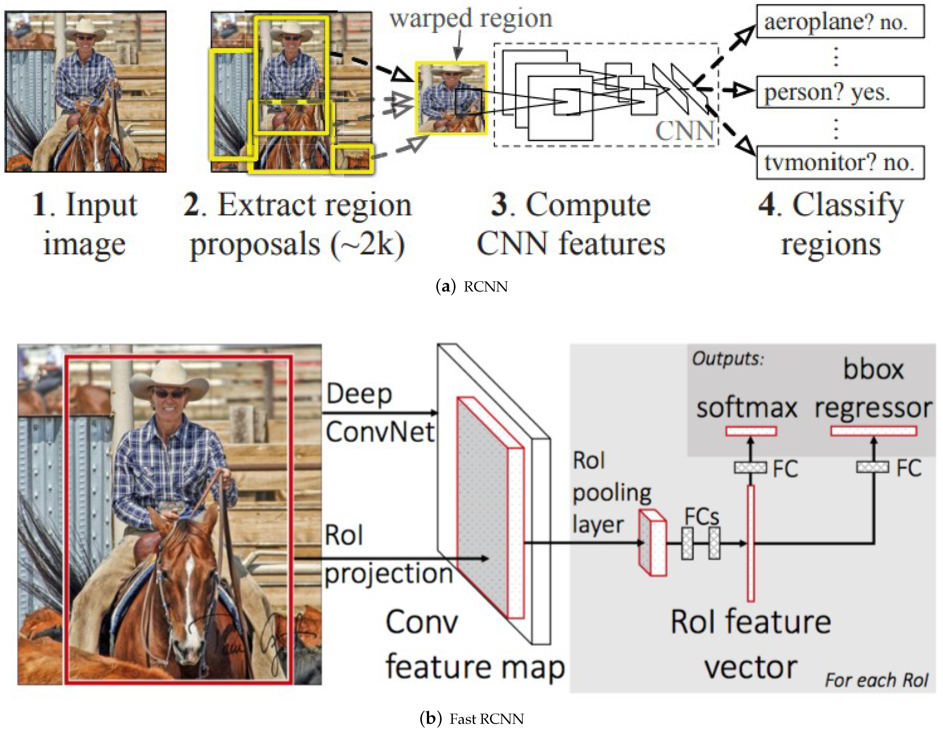
2.2.1. RCNN Family
2.2.2. YOLO Family
- BackBone: It consists of a convolutional neural network that gathers and generates visual features of various sizes and shapes. The feature extractors employed are classification models such as ResNet, VGG, and EfficientNet.
- Neck: A group of layers that combine and mix traits before sending them to the prediction layer.
- Head: Combines the predictions from the bounding box with features from the neck. The features and bounding box coordinates are subjected to classification and regression in order to complete the detection procedure. normally produces 4 values, including width, height, and x, y coordinates.
- YOLOv2: [96] overcomes the limitations in the previous version by replacing the backbone architecture with DarkNet19 which results in faster detection with mAP of 78.6% on 544 × 544 resolution images from PASCAL VOC 2007 dataset. Moreover, out of the some improvements in this version compared to the predecessor, the first one is the addition of batch normalization layer for enhanced stability in the network. Secondly, the replacement of grid boxes with anchor box which allows the prediction of multiple objects. The ratio of overlap over union IoU between the predetermined anchor box and the anticipated bounding box is calculated. The IoU value is a threshold used to determine whether or not the likelihood of the identified object is high enough to make a forecast.
- YOLOv3: The same authors published their updated algorithm [103] in 2018. The Darknet-53 architecture served as its foundation. Newer version introduced the idea of Feature Pyramid Network (FPN) for multiple feature extraction for an image.
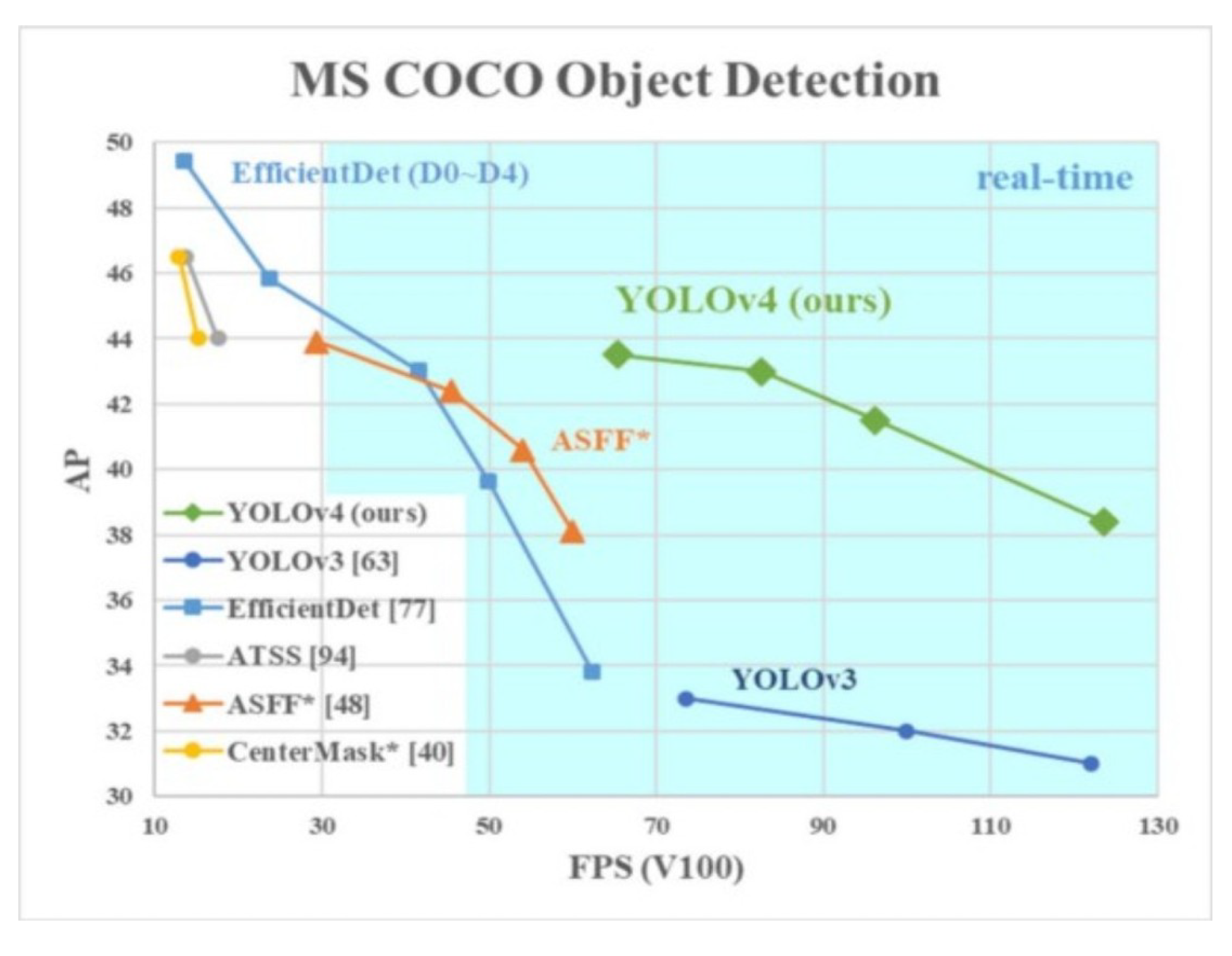
- YOLOv4: The bag of freebies and bag of specials concepts were introduced in YOLOv4 [104] as methods for improving model performance without raising the cost of inference. However, the author of YOLOv4 did experiment on three different backbone architectures including, CSPDarknet533, CSPResNext50 and EfficientNet-B3. The bag of specials allows the selection of additional modules in the neck such as Special Attention Module (SAM), Special Pyramid Pooling (SPP) and Path Aggregation Network (PAN).
2.2.3. RetinaNet
3. Literature Review
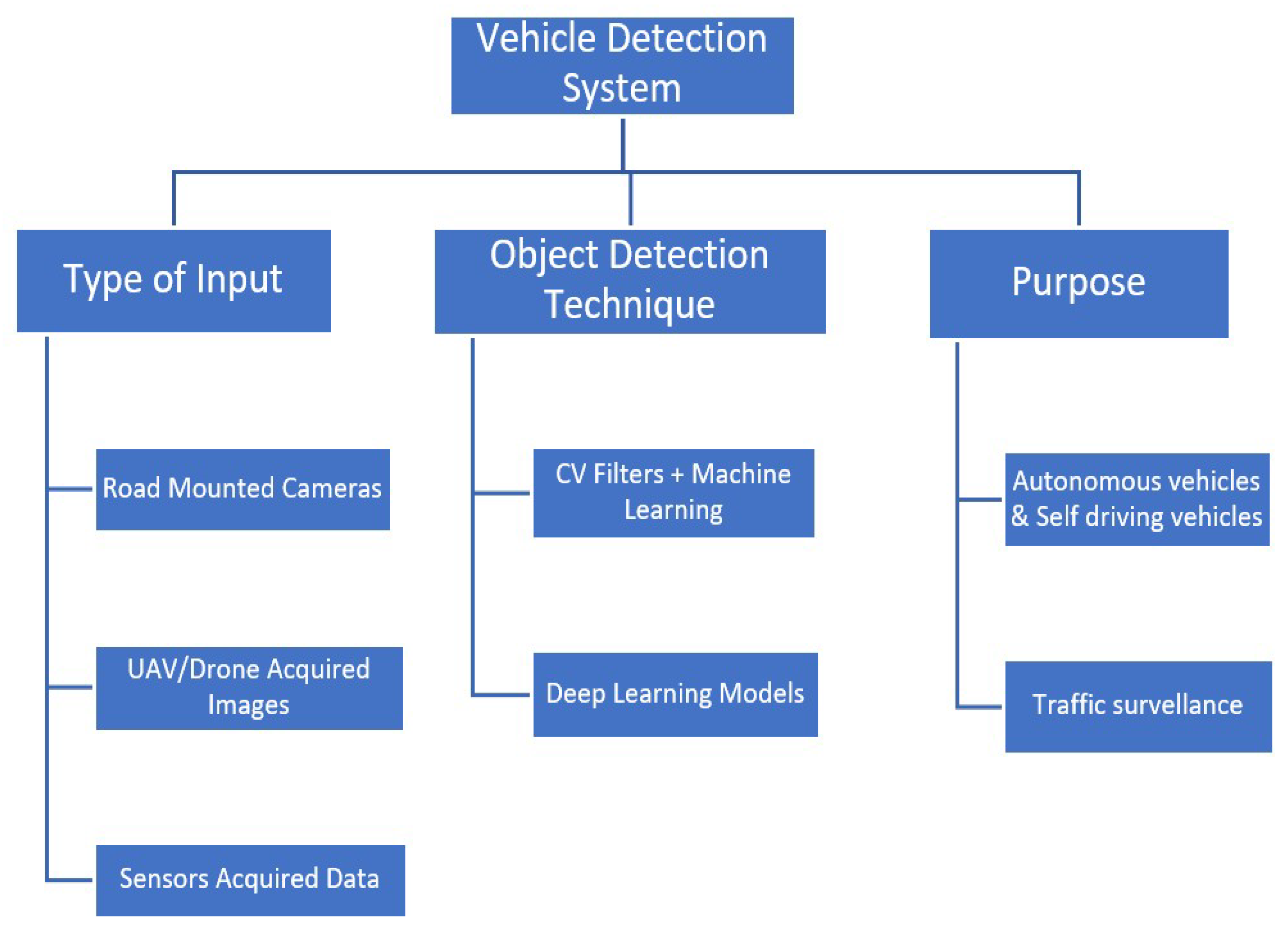
- Classification based on type of input:
- (a)
- surveillance cameras acquired images and videos;
- (b)
- UAV acquired images and videos;
- (c)
- sensors acquired data (e.g., Lidar and Radar).
- Classification based on object detection techniques:
- (a)
- detection using Image processing with machine learning;
- (b)
- deep learning-based systems.
- i
- Two Stage Detector;
- ii
- One Stage Detector;
- iii
- Hybrid Models.
- Classification based on purpose
- (a)
- Autonomous Vehicles and Self driving vehicles
- (b)
- Traffic Surveillance
- We address the problem of vehicle detection in varying and harsh weather condition where the problem of low visibility is addressed by using a image restoration module.
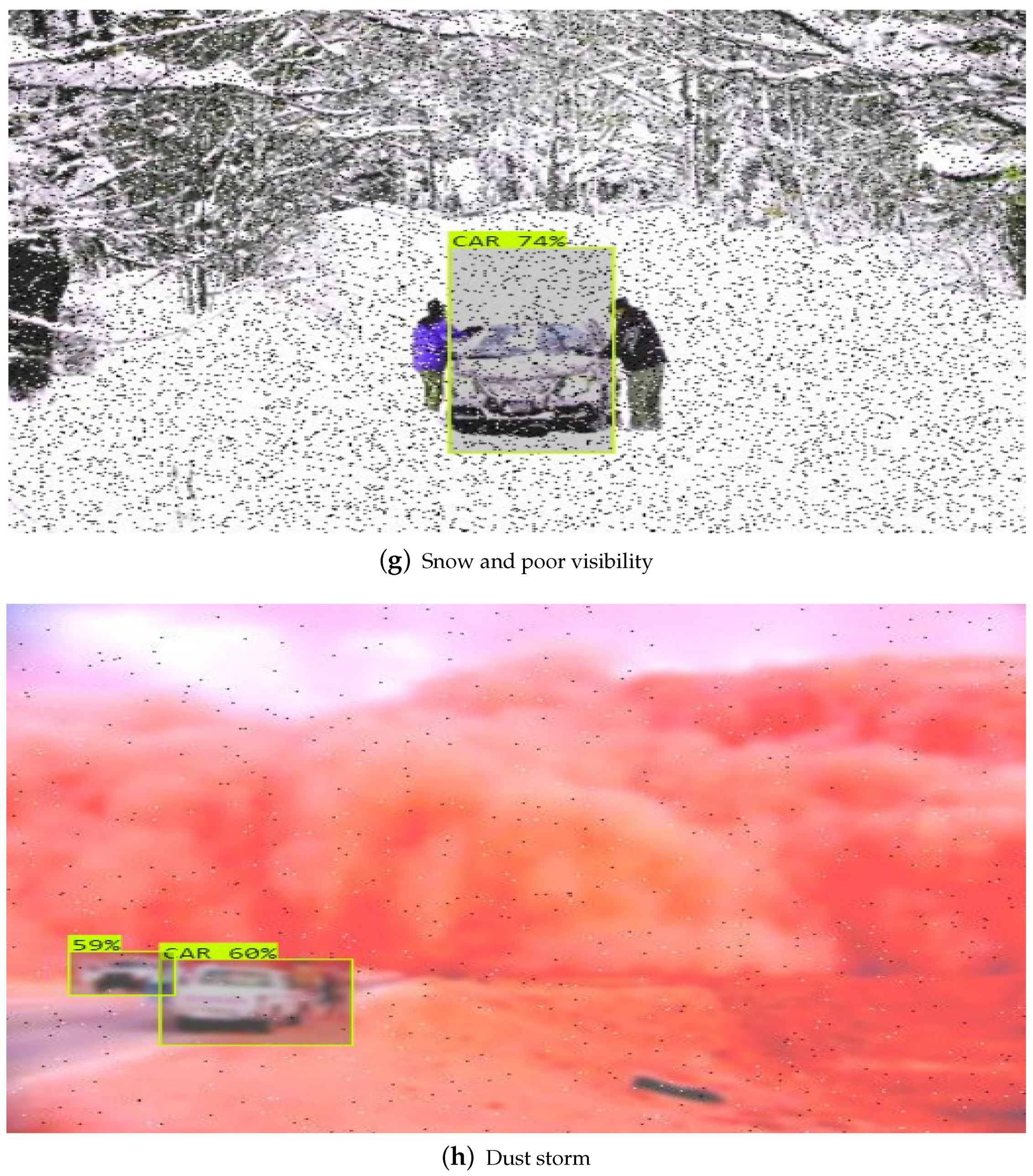
- We use YOLOv4 as backbone architecture for the detection of vehicles in six difficult weather conditions including haze, sandstorm, snowstorm, fog, dust, rain both in day and night.
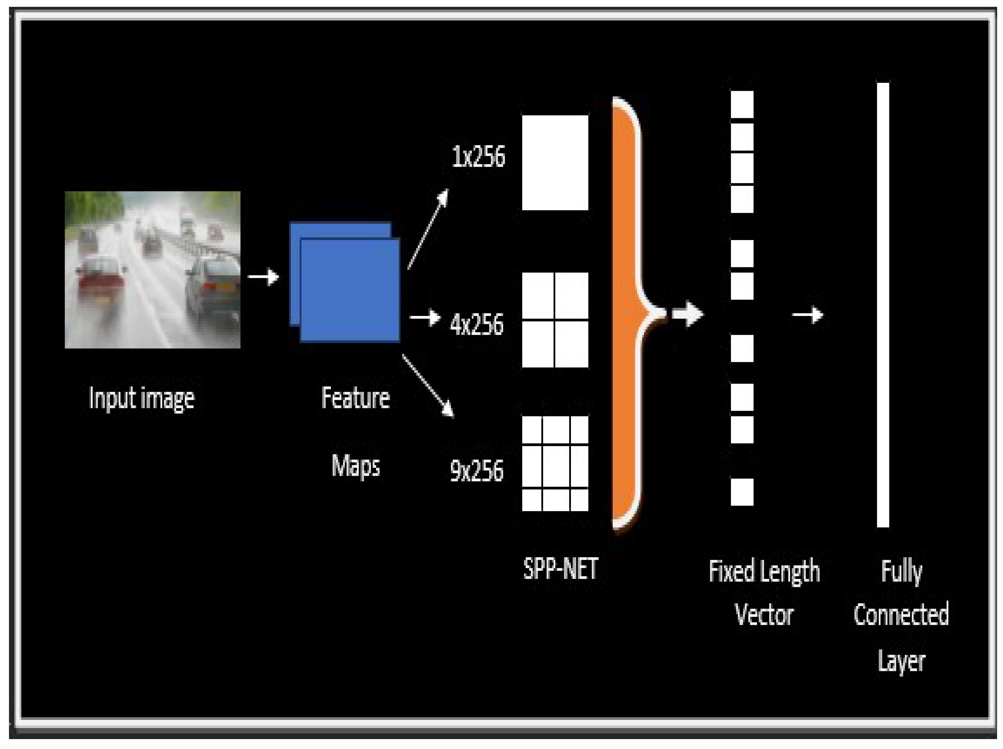
- We address the problem of detection far away and small size vehicles through the addition of double Spatial Pyramid Pooling Network after the last convolution layer [122].
- For capturing vehicle’s fine grained information we add an extra attention module before the convolution layer in the backbone architecture.
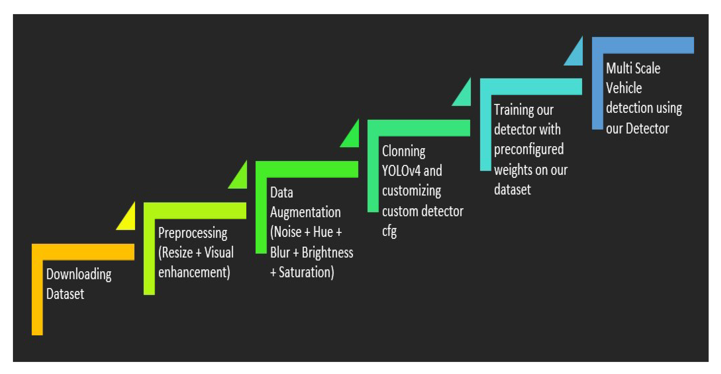
4. Materials and Methods
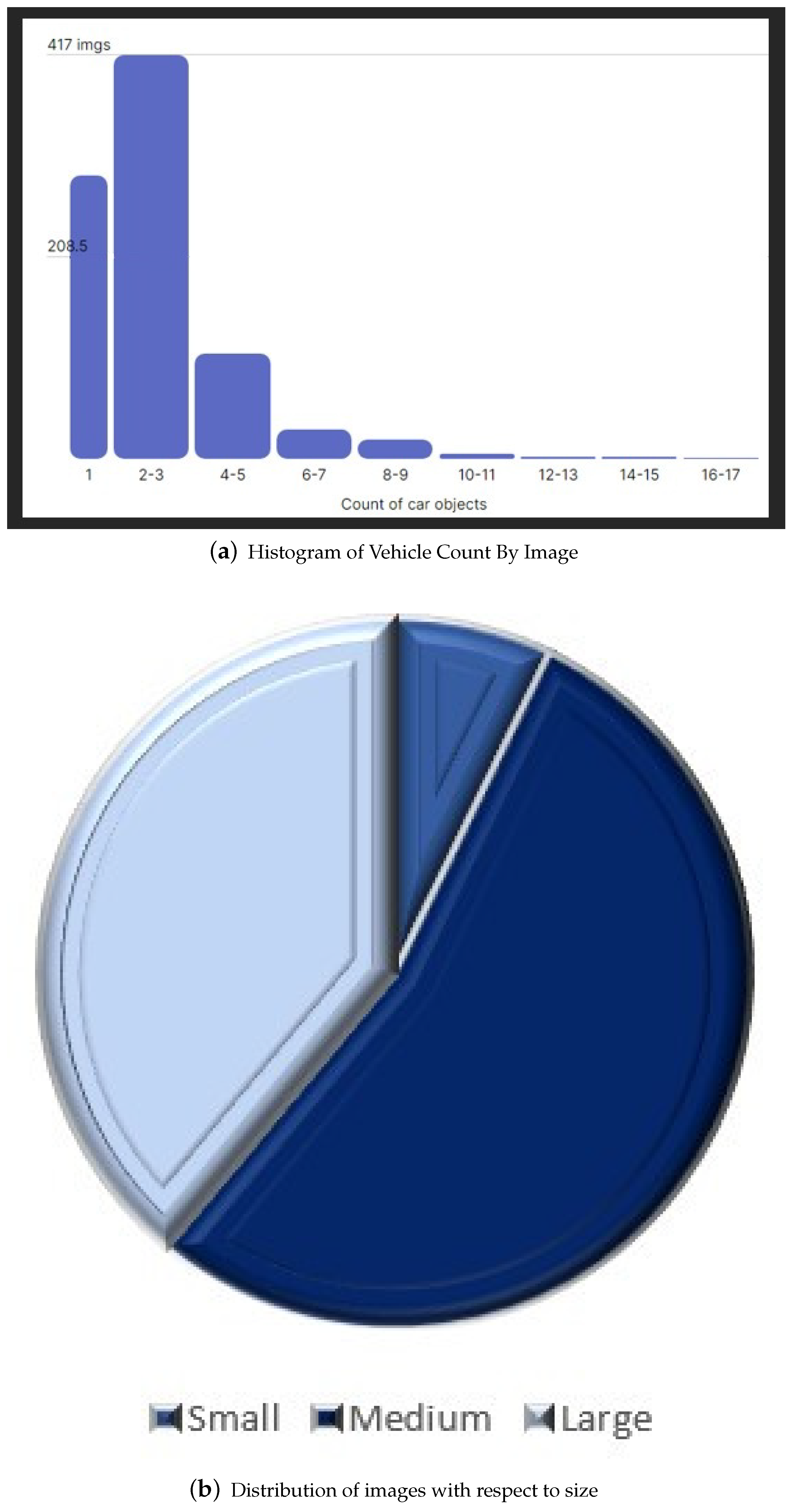
4.1. Dataset
4.2. Data Annotation
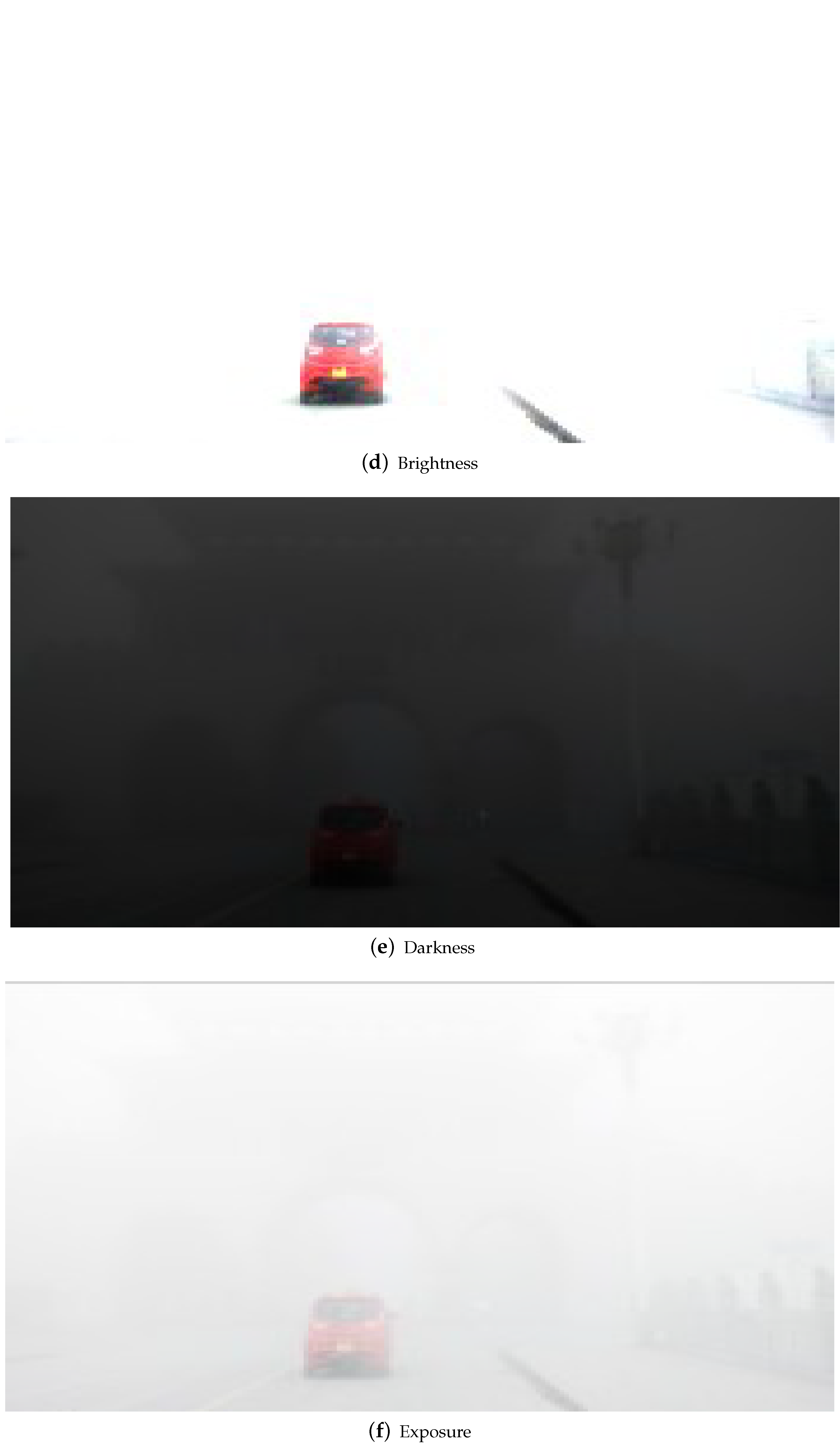
4.3. Data Augmentation
4.3.1. Hue
4.3.2. Saturation
4.3.3. Brightness
4.3.4. Exposure
4.3.5. Blur
4.3.6. Noise
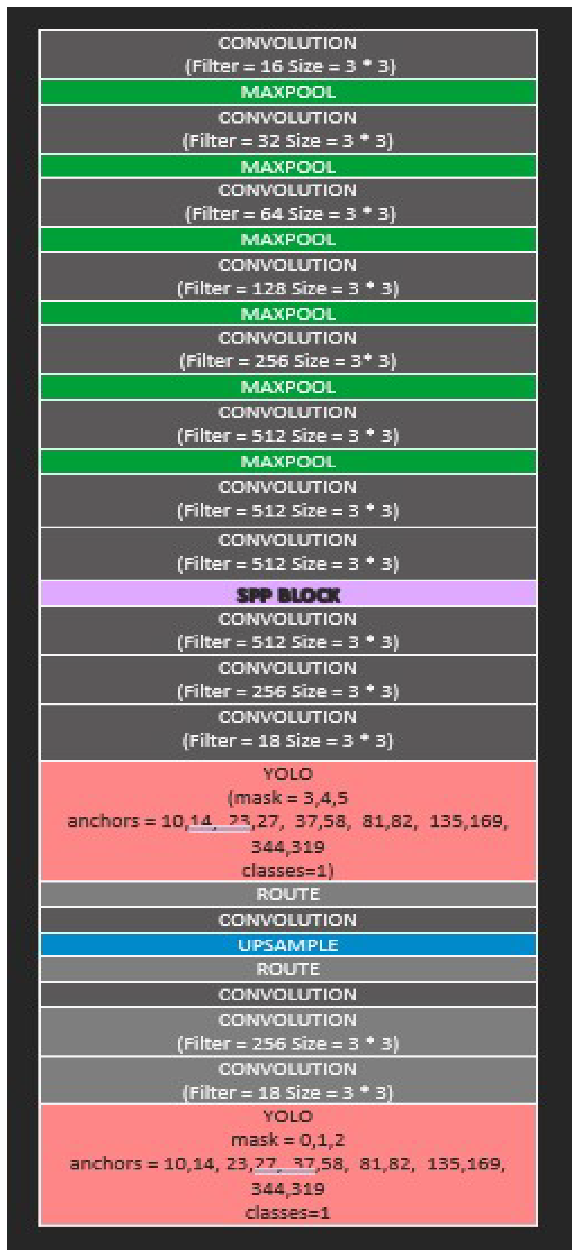
4.4. Customized Yolov4 Detector
4.4.1. Overall Model Design
4.4.2. CSPDarknet53 as Backbone Network
4.4.3. Adding Spatial Pyramid Pooling Block
4.4.4. Removing Batch Normalization
5. Experimental Analysis
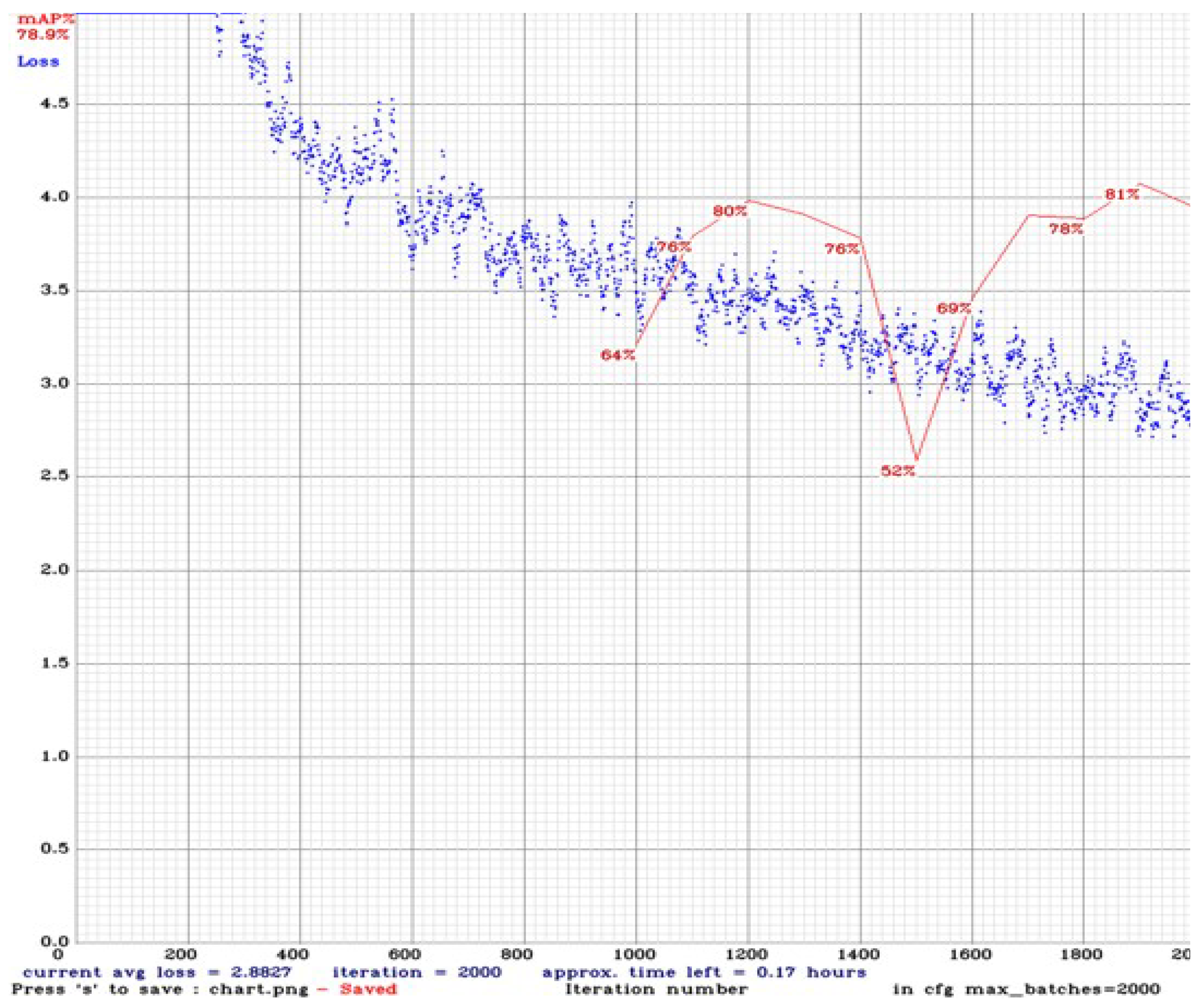
5.1. Training Setup
5.2. Evaluation of the Detector
- Confidence Score: It displays the likelihood that bounding box holds a vehicle. It is predicted by the last layer of the detector, i.e., a classifier.
- Intersection over Union (IoU): This metric counts the area encompassed by Actual bounding box (Ba) and predicted bounding box (Bp), We used a predefined threshold value of 0.5 for single class to classify if the prediction is false or true positive.
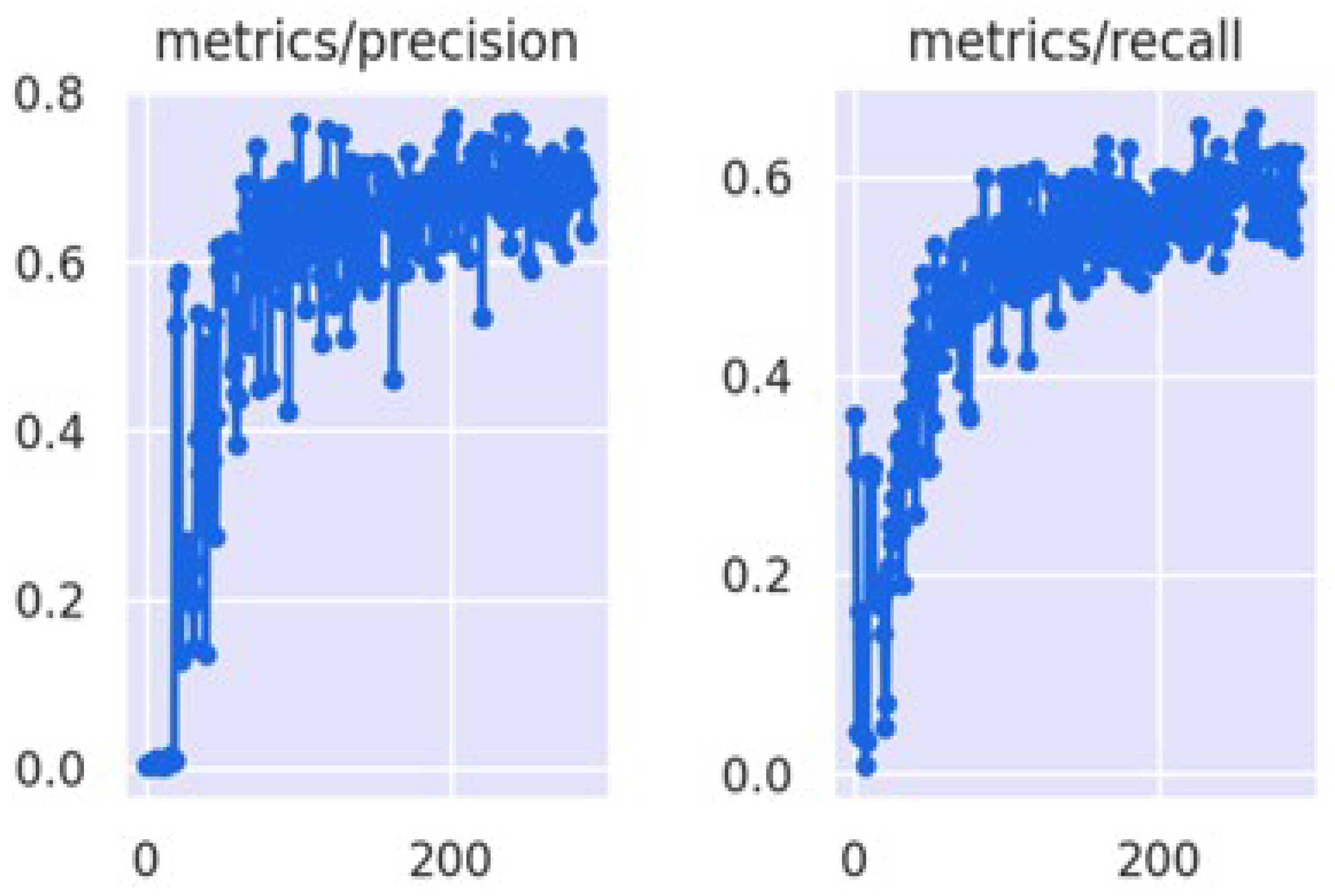
- Precision: is the ratio of total true positive and sum of true positive and false positive.
- Recall: is the ratio of true positives and sum of true positive and false negative.
- Minimum Average Precision (mAP@0.5):
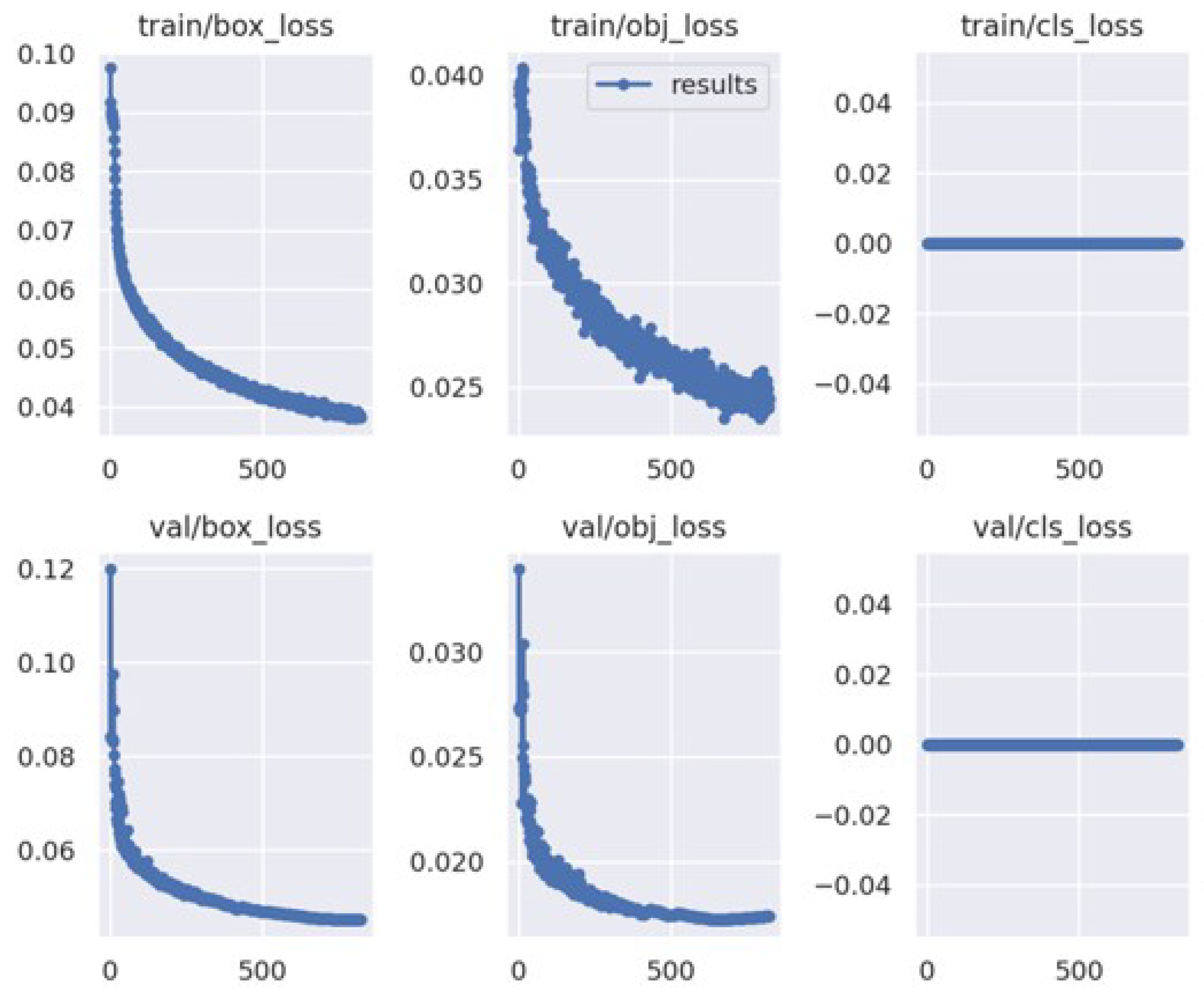
5.2.1. Results
5.2.2. Result Comparison and Discussion
6. Conclusions
Author Contributions
Funding
Institutional Review Board Statement
Informed Consent Statement
Data Availability Statement
Conflicts of Interest
References
- Chen, L.; Li, S.; Bai, Q.; Yang, J.; Jiang, S.; Miao, Y. Review of image classification algorithms based on convolutional neural networks. Remote. Sens. 2021, 13, 4712. [Google Scholar] [CrossRef]
- Khairandish, M.; Sharma, M.; Jain, V.; Chatterjee, J.; Jhanjhi, N. A hybrid CNN-SVM threshold segmentation approach for tumor detection and classification of MRI brain images. IRBM 2021, 43, 290–299. [Google Scholar] [CrossRef]
- Humayun, M.; Sujatha, R.; Almuayqil, S.N.; Jhanjhi, N. A Transfer Learning Approach with a Convolutional Neural Network for the Classification of Lung Carcinoma. Healthcare 2022, 10, 1058. [Google Scholar] [CrossRef]
- He, T.; Zhang, Z.; Zhang, H.; Zhang, Z.; Xie, J.; Li, M. Bag of tricks for image classification with convolutional neural networks. In Proceedings of the IEEE/CVF Conference on Computer Vision and Pattern Recognition, Nashville, TN, USA, 20–25 June 2019; pp. 558–567. [Google Scholar]
- Mahmood, A.; Bennamoun, M.; An, S.; Sohel, F.A.; Boussaid, F.; Hovey, R.; Kendrick, G.A.; Fisher, R.B. Deep image representations for coral image classification. IEEE J. Ocean. Eng. 2018, 44, 121–131. [Google Scholar] [CrossRef]
- Yap, J.; Yolland, W.; Tschandl, P. Multimodal skin lesion classification using deep learning. Exp. Dermatol. 2018, 27, 1261–1267. [Google Scholar] [CrossRef] [PubMed]
- Sharma, R.; Singh, A.; Kavita; Jhanjhi, N.; Masud, M.; Jaha, E.S.; Verma, S. Plant Disease Diagnosis and Image Classification Using Deep Learning. CMC Comput. Mater. Contin. 2022, 71, 2125–2140. [Google Scholar] [CrossRef]
- Khalid, N.; Shahrol, N.A. Evaluation the accuracy of oil palm tree detection using deep learning and support vector machine classifiers. In Proceedings of the IOP Conference Series: Earth and Environmental Science, Tashkent, Uzbekistan, 18–20 May 2022; IOP Publishing: Bristol, UK, 2022; Volume 1051, p. 12028. [Google Scholar]
- Saeed, S.; Jhanjhi, N.Z.; Naqvi, M.; Humyun, M.; Ahmad, M.; Gaur, L. Optimized Breast Cancer Premature Detection Method with Computational Segmentation: A Systematic Review Mapping. Approaches Appl. Deep. Learn. Virtual Med. Care 2022, 24–51. [Google Scholar] [CrossRef]
- Khalil, M.I.; Humayun, M.; Jhanjhi, N.; Talib, M.; Tabbakh, T.A. Multi-class segmentation of organ at risk from abdominal CT images: A deep learning approach. In Intelligent Computing and Innovation on Data Science; Springer: Berlin/Heidelberg, Germany, 2021; pp. 425–434. [Google Scholar]
- Dash, S.; Verma, S.; Kavita; Jhanjhi, N.; Masud, M.; Baz, M. Curvelet Transform Based on Edge Preserving Filter for Retinal Blood Vessel Segmentation. CMC Comput. Mater. Contin. 2022, 71, 2459–2476. [Google Scholar] [CrossRef]
- Deng, J.; Zhong, Z.; Huang, H.; Lan, Y.; Han, Y.; Zhang, Y. Lightweight semantic segmentation network for real-time weed mapping using unmanned aerial vehicles. Appl. Sci. 2020, 10, 7132. [Google Scholar] [CrossRef]
- Hofmarcher, M.; Unterthiner, T.; Arjona-Medina, J.; Klambauer, G.; Hochreiter, S.; Nessler, B. Visual scene understanding for autonomous driving using semantic segmentation. In Explainable AI: Interpreting, Explaining and Visualizing Deep Learning; Springer: Berlin/Heidelberg, Germany, 2019; pp. 285–296. [Google Scholar]
- Tan, M.; Le, Q. Efficientnet: Rethinking model scaling for convolutional neural networks. In Proceedings of the International Conference on Machine Learning, Nanchang, China, 21–23 June 2019; pp. 6105–6114. [Google Scholar]
- Carion, N.; Massa, F.; Synnaeve, G.; Usunier, N.; Kirillov, A.; Zagoruyko, S. End-to-end object detection with transformers. In Proceedings of the European Conference on Computer Vision, Glasgow, UK, 23–28 August 2020; Springer: Berlin/Heidelberg, Germany, 2020; pp. 213–229. [Google Scholar]
- Gouda, W.; Sama, N.U.; Al-Waakid, G.; Humayun, M.; Jhanjhi, N.Z. Detection of Skin Cancer Based on Skin Lesion Images Using Deep Learning. Healthcare 2022, 10, 1183. [Google Scholar] [CrossRef]
- Ramamoorthy, M.; Qamar, S.; Manikandan, R.; Jhanjhi, N.Z.; Masud, M.; AlZain, M.A. Earlier Detection of Brain Tumor by Pre-Processing Based on Histogram Equalization with Neural Network. Healthcare 2022, 10, 1218. [Google Scholar] [CrossRef] [PubMed]
- Saeed, S.; Abdullah, A.; Jhanjhi, N.; Naqvi, M.; Nayyar, A. New techniques for efficiently k-NN algorithm for brain tumor detection. Multimed. Tools Appl. 2022, 81, 18595–18616. [Google Scholar] [CrossRef]
- Attaullah, M.; Ali, M.; Almufareh, M.F.; Ahmad, M.; Hussain, L.; Jhanjhi, N.; Humayun, M. Initial Stage COVID-19 Detection System Based on Patients’ Symptoms and Chest X-Ray Images. Appl. Artif. Intell. 2022, 36, 1–20. [Google Scholar] [CrossRef]
- Oh, S.W.; Lee, J.Y.; Xu, N.; Kim, S.J. Video object segmentation using space-time memory networks. In Proceedings of the IEEE/CVF International Conference on Computer Vision, Seoul, Korea, 27 October–2 November 2019; pp. 9226–9235. [Google Scholar]
- Sagues-Tanco, R.; Benages-Pardo, L.; López-Nicolás, G.; Llorente, S. Fast synthetic dataset for kitchen object segmentation in deep learning. IEEE Access 2020, 8, 220496–220506. [Google Scholar] [CrossRef]
- Wu, B.; Wan, A.; Yue, X.; Keutzer, K. Squeezeseg: Convolutional neural nets with recurrent crf for real-time road-object segmentation from 3d lidar point cloud. In Proceedings of the 2018 IEEE International Conference on Robotics and Automation (ICRA), Brisbane, QL, Australia, 21–25 May 2018; pp. 1887–1893. [Google Scholar]
- Liu, X.; Dai, B.; He, H. Real-time object segmentation for visual object detection in dynamic scenes. In Proceedings of the 2011 International Conference of Soft Computing and Pattern Recognition (SoCPaR), Dalian, China, 14–16 October 2011; pp. 423–428. [Google Scholar]
- Chen, Z.; Zhang, Z.; Bu, Y.; Dai, F.; Fan, T.; Wang, H. Underwater object segmentation based on optical features. Sensors 2018, 18, 196. [Google Scholar] [CrossRef]
- Gu, J.; Bellone, M.; Sell, R.; Lind, A. Object segmentation for autonomous driving using iseAuto data. Electronics 2022, 11, 1119. [Google Scholar] [CrossRef]
- Fukuda, M.; Okuno, T.; Yuki, S. Central Object Segmentation by Deep Learning to Continuously Monitor Fruit Growth through RGB Images. Sensors 2021, 21, 6999. [Google Scholar] [CrossRef]
- Kim, B.; Lee, J.; Kang, J.; Kim, E.S.; Kim, H.J. Hotr: End-to-end human-object interaction detection with transformers. In Proceedings of the IEEE/CVF Conference on Computer Vision and Pattern Recognition, Nashville, TN, USA, 20–25 June 2021; pp. 74–83. [Google Scholar]
- Yao, B.; Fei-Fei, L. Recognizing human-object interactions in still images by modeling the mutual context of objects and human poses. IEEE Trans. Pattern Anal. Mach. Intell. 2012, 34, 1691–1703. [Google Scholar]
- Zheng, C.; Zhu, S.; Mendieta, M.; Yang, T.; Chen, C.; Ding, Z. 3d human pose estimation with spatial and temporal transformers. In Proceedings of the IEEE/CVF International Conference on Computer Vision, Nashville, TN, USA, 20–25 June 2021; pp. 11656–11665. [Google Scholar]
- Tompson, J.J.; Jain, A.; LeCun, Y.; Bregler, C. Joint training of a convolutional network and a graphical model for human pose estimation. Adv. Neural Inf. Process. Syst. 2014, 27, 1799–1807. [Google Scholar]
- Araújo, V.M.; Shukla, A.; Chion, C.; Gambs, S.; Michaud, R. Machine-Learning Approach for Automatic Detection of Wild Beluga Whales from Hand-Held Camera Pictures. Sensors 2022, 22, 4107. [Google Scholar] [CrossRef]
- Sharma, N.; Scully-Power, P.; Blumenstein, M. Shark detection from aerial imagery using region-based CNN, a study. In Proceedings of the Australasian Joint Conference on Artificial Intelligence, Wellington, New Zealand, 11–14 December 2018; Springer: Berlin/Heidelberg, Germany, 2018; pp. 224–236. [Google Scholar]
- Tang, Y.; Wang, J.; Wang, X.; Gao, B.; Dellandréa, E.; Gaizauskas, R.; Chen, L. Visual and semantic knowledge transfer for large scale semi-supervised object detection. IEEE Trans. Pattern Anal. Mach. Intell. 2017, 40, 3045–3058. [Google Scholar] [CrossRef] [PubMed]
- Sujatha, R.; Chatterjee, J.M.; Jhanjhi, N.; Brohi, S.N. Performance of deep learning vs. machine learning in plant leaf disease detection. Microprocess. Microsyst. 2021, 80, 103615. [Google Scholar] [CrossRef]
- Asmar, D.C.; Zelek, J.S.; Abdallah, S.M. Seeing the trees before the forest [natural object detection]. In Proceedings of the 2nd Canadian Conference on Computer and Robot Vision (CRV’05), Victoria, BC, Canada, 9–11 May 2005; pp. 587–593. [Google Scholar]
- Oh, S.; Chang, A.; Ashapure, A.; Jung, J.; Dube, N.; Maeda, M.; Gonzalez, D.; Landivar, J. Plant counting of cotton from UAS imagery using deep learning-based object detection framework. Remote. Sens. 2020, 12, 2981. [Google Scholar] [CrossRef]
- Kusumo, B.S.; Heryana, A.; Mahendra, O.; Pardede, H.F. Machine learning-based for automatic detection of corn-plant diseases using image processing. In Proceedings of the 2018 International Conference on Computer, Control, Informatics and Its Applications (IC3INA), Tangerang, Indonesia, 1–2 November 2018; pp. 93–97. [Google Scholar]
- Khan, N.A.; Jhanjhi, N.; Brohi, S.N.; Usmani, R.S.A.; Nayyar, A. Smart traffic monitoring system using unmanned aerial vehicles (UAVs). Comput. Commun. 2020, 157, 434–443. [Google Scholar] [CrossRef]
- Alkinani, M.H.; Almazroi, A.A.; Jhanjhi, N.; Khan, N.A. 5G and IoT based reporting and accident detection (RAD) system to deliver first aid box using unmanned aerial vehicle. Sensors 2021, 21, 6905. [Google Scholar] [CrossRef]
- Song, H.; Liang, H.; Li, H.; Dai, Z.; Yun, X. Vision-based vehicle detection and counting system using deep learning in highway scenes. Eur. Transp. Res. Rev. 2019, 11, 1–16. [Google Scholar] [CrossRef]
- Arabi, S.; Haghighat, A.; Sharma, A. A deep-learning-based computer vision solution for construction vehicle detection. Comput. Aided Civ. Infrastruct. Eng. 2020, 35, 753–767. [Google Scholar] [CrossRef]
- Wang, H.; Wang, H.; Xu, K. Evolutionary recurrent neural network for image captioning. Neurocomputing 2020, 401, 249–256. [Google Scholar] [CrossRef]
- Alzubi, J.A.; Jain, R.; Nagrath, P.; Satapathy, S.; Taneja, S.; Gupta, P. Deep image captioning using an ensemble of CNN and LSTM based deep neural networks. J. Intell. Fuzzy Syst. 2021, 40, 5761–5769. [Google Scholar] [CrossRef]
- Amirian, S.; Rasheed, K.; Taha, T.R.; Arabnia, H.R. Image captioning with generative adversarial network. In Proceedings of the 2019 International Conference on Computational Science and Computational Intelligence (CSCI), Las Vegas, NV, USA, 5–7 December 2019; pp. 272–275. [Google Scholar]
- Shi, H.; Li, P.; Wang, B.; Wang, Z. Image captioning based on deep reinforcement learning. In Proceedings of the 10th International Conference on Internet Multimedia Computing and Service, Nanjing, China, 17–19 August 2018; pp. 1–5. [Google Scholar]
- Ullah, A.; Ishaq, N.; Azeem, M.; Ashraf, H.; Jhanjhi, N.; Humayun, M.; Tabbakh, T.A.; Almusaylim, Z.A. A survey on continuous object tracking and boundary detection schemes in IoT assisted wireless sensor networks. IEEE Access 2021, 9, 126324–126336. [Google Scholar] [CrossRef]
- Wang, Q.; Zhang, L.; Bertinetto, L.; Hu, W.; Torr, P.H. Fast online object tracking and segmentation: A unifying approach. In Proceedings of the IEEE/CVF Conference on Computer Vision and Pattern Recognition, Nashville, TN, USA, 20–25 June 2019; pp. 1328–1338. [Google Scholar]
- Meinhardt, T.; Kirillov, A.; Leal-Taixe, L.; Feichtenhofer, C. Trackformer: Multi-object tracking with transformers. In Proceedings of the IEEE/CVF Conference on Computer Vision and Pattern Recognition, Nashville, TN, USA, 20–25 June 2022; pp. 8844–8854. [Google Scholar]
- Kristan, M.; Leonardis, A.; Matas, J.; Felsberg, M.; Pflugfelder, R.; Kämäräinen, J.K.; Danelljan, M.; Zajc, L.Č.; Lukežič, A.; Drbohlav, O.; et al. The eighth visual object tracking VOT2020 challenge results. In Proceedings of the European Conference on Computer Vision, Glasgow, UK, 23–28 August 2020; Springer: Berlin/Heidelberg, Germany, 2020; pp. 547–601. [Google Scholar]
- Wang, Y.; Xu, Z.; Wang, X.; Shen, C.; Cheng, B.; Shen, H.; Xia, H. End-to-end video instance segmentation with transformers. In Proceedings of the IEEE/CVF Conference on Computer Vision and Pattern Recognition, Nashville, TN, USA, 20–25 June 2021; pp. 8741–8750. [Google Scholar]
- Tian, Z.; Shen, C.; Chen, H. Conditional convolutions for instance segmentation. In Proceedings of the European Conference on Computer Vision, Glasgow, UK, 23–28 August 2020; Springer: Berlin/Heidelberg, Germany, 2020; pp. 282–298. [Google Scholar]
- Bolya, D.; Zhou, C.; Xiao, F.; Lee, Y.J. Yolact: Real-time instance segmentation. In Proceedings of the IEEE/CVF International Conference on Computer Vision, Seoul, Korea, 27 October–2 November 2019; pp. 9157–9166. [Google Scholar]
- Yang, Y.; Li, G.; Wu, Z.; Su, L.; Huang, Q.; Sebe, N. Reverse perspective network for perspective-aware object counting. In Proceedings of the IEEE/CVF Conference on Computer Vision and Pattern Recognition, Seattle, WA, USA, 13–19 June 2020; pp. 4374–4383. [Google Scholar]
- Rahutomo, R.; Perbangsa, A.S.; Lie, Y.; Cenggoro, T.W.; Pardamean, B. Artificial intelligence model implementation in web-based application for pineapple object counting. In Proceedings of the 2019 International Conference on Information Management and Technology (ICIMTech), Jakarta, Indonesia, 19–20 August 2019; Volume 1, pp. 525–530. [Google Scholar]
- Zhang, S.; Li, H.; Kong, W. Object counting method based on dual attention network. IET Image Process. 2020, 14, 1621–1627. [Google Scholar] [CrossRef]
- Dirir, A.; Ignatious, H.; Elsayed, H.; Khan, M.; Adib, M.; Mahmoud, A.; Al-Gunaid, M. An Advanced Deep Learning Approach for Multi-Object Counting in Urban Vehicular Environments. Future Internet 2021, 13, 306. [Google Scholar] [CrossRef]
- Chayeb, A.; Ouadah, N.; Tobal, Z.; Lakrouf, M.; Azouaoui, O. HOG based multi-object detection for urban navigation. In Proceedings of the 17th International IEEE Conference on Intelligent Transportation Systems (ITSC), Qingdao, China, 8–11 October 2014; pp. 2962–2967. [Google Scholar] [CrossRef]
- Yamauchi, Y.; Matsushima, C.; Yamashita, T.; Fujiyoshi, H. Relational HOG feature with wild-card for object detection. In Proceedings of the 2011 IEEE International Conference on Computer Vision Workshop (ICCV Workshops), Venice, Italy, 22–29 October 2011; pp. 1785–1792. [Google Scholar] [CrossRef]
- Dong, L.; Yu, X.; Li, L.; Hoe, J.K.E. HOG based multi-stage object detection and pose recognition for service robot. In Proceedings of the 2010 11th International Conference on Control Automation Robotics & Vision, Singapore, 7–10 December 2010; pp. 2495–2500. [Google Scholar]
- Cheng, G.; Zhou, P.; Yao, X.; Yao, C.; Zhang, Y.; Han, J. Object detection in VHR optical remote sensing images via learning rotation-invariant HOG feature. In Proceedings of the 2016 4th International Workshop on Earth Observation and Remote Sensing Applications (EORSA), Guangzhou, China, 4–6 July 2016; pp. 433–436. [Google Scholar] [CrossRef]
- Ren, H.; Li, Z.N. Object detection using edge histogram of oriented gradient. In Proceedings of the 2014 IEEE International Conference on Image Processing (ICIP), Paris, France, 27–30 October 2014; pp. 4057–4061. [Google Scholar]
- Han, F.; Shan, Y.; Cekander, R.; Sawhney, H.S.; Kumar, R. A two-stage approach to people and vehicle detection with hog-based svm. In Proceedings of the Performance Metrics for Intelligent Systems 2006 Workshop, Washington, DC, USA, 11–13 October 2006; pp. 133–140. [Google Scholar]
- Dalal, N.; Triggs, B. Histograms of oriented gradients for human detection, 2005. In Proceedings of the IEEE Computer Vision and Pattern Recognition, San Diego, CA, USA, 21–23 September 2005. [Google Scholar]
- Viola, P.; Jones, M. Rapid object detection using a boosted cascade of simple features. In Proceedings of the 2001 IEEE Computer Society Conference on Computer Vision and Pattern Recognition, CVPR 2001, Kauai, HI, USA, 8–14 December 2001; Volume 1, p. 1. [Google Scholar]
- Li, Y.L.; Wang, S. HAR-Net: Joint learning of hybrid attention for single-stage object detection. arXiv 2019, arXiv:1904.11141. [Google Scholar] [CrossRef] [PubMed]
- Soo, S. Object Detection Using Haar-Cascade Classifier; Institute of Computer Science, University of Tartu: Tartu, Estonia, 2014; Volume 2, pp. 1–12. [Google Scholar]
- Jalled, F.; Voronkov, I. Object detection using image processing. arXiv 2016, arXiv:1611.07791. [Google Scholar]
- Cuimei, L.; Zhiliang, Q.; Nan, J.; Jianhua, W. Human face detection algorithm via Haar cascade classifier combined with three additional classifiers. In Proceedings of the 2017 13th IEEE International Conference on Electronic Measurement & Instruments (ICEMI), Yangzhou, China, 20–23 October 2017; pp. 483–487. [Google Scholar]
- Pawełczyk, M.; Wojtyra, M. Real world object detection dataset for quadcopter unmanned aerial vehicle detection. IEEE Access 2020, 8, 174394–174409. [Google Scholar] [CrossRef]
- Whitehill, J.; Omlin, C.W. Haar features for FACS AU recognition. In Proceedings of the 7th International Conference on Automatic Face and Gesture Recognition (FGR06), Southampton, UK, 10–12 April 2006; p. 5. [Google Scholar]
- Haselhoff, A.; Kummert, A. A vehicle detection system based on haar and triangle features. In Proceedings of the 2009 IEEE Intelligent Vehicles Symposium, Xi’an, China, 3–5 June 2009; pp. 261–266. [Google Scholar]
- Chen, D.S.; Liu, Z.K. Generalized Haar-like features for fast face detection. In Proceedings of the 2007 International Conference on Machine Learning and Cybernetics, Cincinnati, OH, USA, 13–15 December 2007; Volume 4, pp. 2131–2135. [Google Scholar]
- Yun, L.; Peng, Z. An automatic hand gesture recognition system based on Viola-Jones method and SVMs. In Proceedings of the 2009 Second International Workshop on Computer Science and Engineering, Qingdao, China, 28–30 October 2009; Volume 2, pp. 72–76. [Google Scholar]
- Sawas, J.; Petillot, Y.; Pailhas, Y. Cascade of boosted classifiers for rapid detection of underwater objects. In Proceedings of the European Conference on Underwater Acoustics, Istambul, Turkey, 5 July 2010; Volume 164. [Google Scholar]
- Nguyen, T.; Park, E.; Han, J.; Park, D.C.; Min, S.Y. Object detection using scale invariant feature transform. In Genetic and Evolutionary Computing; Springer: Berlin/Heidelberg, Germany, 2014; pp. 65–72. [Google Scholar]
- Geng, C.; Jiang, X. SIFT features for face recognition. In Proceedings of the 2009 2nd IEEE International Conference on Computer Science and Information Technology, Beijing, China, 8–11 August 2009; pp. 598–602. [Google Scholar]
- Piccinini, P.; Prati, A.; Cucchiara, R. Real-time object detection and localization with SIFT-based clustering. Image Vis. Comput. 2012, 30, 573–587. [Google Scholar] [CrossRef]
- Zhao, W.L.; Ngo, C.W. Flip-invariant SIFT for copy and object detection. IEEE Trans. Image Process. 2012, 22, 980–991. [Google Scholar] [CrossRef]
- Najva, N.; Bijoy, K.E. SIFT and tensor based object detection and classification in videos using deep neural networks. Procedia Comput. Sci. 2016, 93, 351–358. [Google Scholar] [CrossRef][Green Version]
- Sun, S.W.; Wang, Y.C.F.; Huang, F.; Liao, H.Y.M. Moving foreground object detection via robust SIFT trajectories. J. Vis. Commun. Image Represent. 2013, 24, 232–243. [Google Scholar] [CrossRef]
- Sakai, Y.; Oda, T.; Ikeda, M.; Barolli, L. An object tracking system based on sift and surf feature extraction methods. In Proceedings of the 2015 18th International Conference on Network-Based Information Systems, Washington, DC, USA, 2–4 September 2015; pp. 561–565. [Google Scholar]
- Chen, Z.; Chen, K.; Chen, J. Vehicle and pedestrian detection using support vector machine and histogram of oriented gradients features. In Proceedings of the 2013 International Conference on Computer Sciences and Applications, Kunming, China, 21–23 September 2013; pp. 365–368. [Google Scholar]
- Anwar, M.A.; Tahir, S.F.; Fahad, L.G.; Kifayat, K.K. Image Forgery Detection by Transforming Local Descriptors into Deep-Derived Features. Available online: https://papers.ssrn.com/sol3/papers.cfm?abstract_id=4134079 (accessed on 3 July 2022).
- Patil, S.; Patil, Y. Face Expression Recognition Using SVM and KNN Classifier with HOG Features. In Proceedings of the International Conference on Computing in Engineering & Technology, Virtual, 12–13 February 2022; Springer: Berlin/Heidelberg, Germany, 2022; pp. 416–424. [Google Scholar]
- Gao, S.; Wei, Y.; Xiong, H. Pedestrian detection algorithm based on improved SLIC segmentation and SVM. In Proceedings of the 2022 IEEE 10th Joint International Information Technology and Artificial Intelligence Conference (ITAIC), Chongqing, China, 17–19 June 2022; Volume 10, pp. 771–775. [Google Scholar]
- Tseng, H.H.; Yang, M.D.; Saminathan, R.; Hsu, Y.C.; Yang, C.Y.; Wu, D.H. Rice Seedling Detection in UAV Images Using Transfer Learning and Machine Learning. Remote. Sens. 2022, 14, 2837. [Google Scholar] [CrossRef]
- Yousef, N.; Parmar, C.; Sata, A. Intelligent inspection of surface defects in metal castings using machine learning. Mater. Today Proc. 2022. [Google Scholar] [CrossRef]
- Sharma, V.; Jain, M.; Jain, T.; Mishra, R. License plate detection and recognition using openCV–python. In Recent Innovations in Computing; Springer: Berlin/Heidelberg, Germany, 2022; pp. 251–261. [Google Scholar]
- Girshick, R.; Donahue, J.; Darrell, T.; Malik, J. Region-based convolutional networks for accurate object detection and segmentation. IEEE Trans. Pattern Anal. Mach. Intell. 2015, 38, 142–158. [Google Scholar] [CrossRef] [PubMed]
- Girshick, R. Fast r-cnn. In Proceedings of the IEEE International Conference on Computer Vision, Santiago, Chile, 7–13 December 2015; pp. 1440–1448. [Google Scholar]
- He, K.; Zhang, X.; Ren, S.; Sun, J. Spatial pyramid pooling in deep convolutional networks for visual recognition. IEEE Trans. Pattern Anal. Mach. Intell. 2015, 37, 1904–1916. [Google Scholar] [CrossRef] [PubMed]
- Ren, S.; He, K.; Girshick, R.; Sun, J. Faster r-cnn: Towards real-time object detection with region proposal networks. Adv. Neural Inf. Process. Syst. 2015, 28. [Google Scholar] [CrossRef] [PubMed]
- He, K.; Zhang, X.; Ren, S.; Sun, J. Deep residual learning for image recognition. In Proceedings of the IEEE Conference on Computer Vision and Pattern Recognition, Las Vegas, NV, USA, 27–30 June 2016; pp. 770–778. [Google Scholar]
- Lin, T.Y.; Dollár, P.; Girshick, R.; He, K.; Hariharan, B.; Belongie, S. Feature pyramid networks for object detection. In Proceedings of the IEEE Conference on Computer Vision and Pattern Recognition, Honolulu, HI, USA, 21–26 July 2017; pp. 2117–2125. [Google Scholar]
- Cai, Z.; Vasconcelos, N. Cascade r-cnn: Delving into high quality object detection. In Proceedings of the IEEE Conference on Computer Vision and Pattern Recognition, Salt Lake City, UT, USA, 18–23 June 2018; pp. 6154–6162. [Google Scholar]
- Redmon, J.; Divvala, S.; Girshick, R.; Farhadi, A. You only look once: Unified, real-time object detection. In Proceedings of the IEEE Conference on Computer Vision and Pattern Recognition, Las Vegas, NV, USA, 27–30 June 2016; pp. 779–788. [Google Scholar]
- Peng, Q.; Luo, W.; Hong, G.; Feng, M.; Xia, Y.; Yu, L.; Hao, X.; Wang, X.; Li, M. Pedestrian detection for transformer substation based on gaussian mixture model and YOLO. In Proceedings of the 2016 8th International Conference on Intelligent Human-Machine Systems and Cybernetics (IHMSC), Zhejiang, China, 11–12 September 2016; Volume 2, pp. 562–565. [Google Scholar]
- Liu, C.; Tao, Y.; Liang, J.; Li, K.; Chen, Y. Object detection based on YOLO network. In Proceedings of the 2018 IEEE 4th Information Technology and Mechatronics Engineering Conference (ITOEC), Chongqing, China, 14–16 December 2018; pp. 799–803. [Google Scholar]
- Fang, W.; Wang, L.; Ren, P. Tinier-YOLO: A real-time object detection method for constrained environments. IEEE Access 2019, 8, 1935–1944. [Google Scholar] [CrossRef]
- Tao, J.; Wang, H.; Zhang, X.; Li, X.; Yang, H. An object detection system based on YOLO in traffic scene. In Proceedings of the 2017 6th International Conference on Computer Science and Network Technology (ICCSNT), Dalian, China, 21–22 October 2017; pp. 315–319. [Google Scholar]
- He, W.; Huang, Z.; Wei, Z.; Li, C.; Guo, B. TF-YOLO: An improved incremental network for real-time object detection. Appl. Sci. 2019, 9, 3225. [Google Scholar] [CrossRef]
- Shafiee, M.J.; Chywl, B.; Li, F.; Wong, A. Fast YOLO: A fast you only look once system for real-time embedded object detection in video. arXiv 2017, arXiv:1709.05943. [Google Scholar] [CrossRef]
- Redmon, J.; Farhadi, A. Yolov3: An incremental improvement. arXiv 2018, arXiv:1804.02767. [Google Scholar]
- Bochkovskiy, A.; Wang, C.Y.; Liao, H.Y.M. Yolov4: Optimal speed and accuracy of object detection. arXiv 2020, arXiv:2004.10934. [Google Scholar]
- Lin, T.Y.; Goyal, P.; Girshick, R.; He, K.; Dollár, P. Focal loss for dense object detection. In Proceedings of the IEEE International Conference on Computer Vision, Venice, Italy, 22–29 October 2017; pp. 2980–2988. [Google Scholar]
- Liu, S.; Wang, J.; Wang, Z.; Yu, B.; Hu, W.; Liu, Y.; Tang, J.; Song, S.L.; Liu, C.; Hu, Y. Brief industry paper: The necessity of adaptive data fusion in infrastructure-augmented autonomous driving system. In Proceedings of the 2022 IEEE 28th Real-Time and Embedded Technology and Applications Symposium (RTAS), Milano, Italy, 4–6 May 2022; pp. 293–296. [Google Scholar]
- Yang, X.; Zou, Y.; Chen, L. Operation analysis of freeway mixed traffic flow based on catch-up coordination platoon. Accid. Anal. Prev. 2022, 175, 106780. [Google Scholar] [CrossRef]
- Munroe, D.T.; Madden, M.G. Multi-class and single-class classification approaches to vehicle model recognition from images. Proc. AICS 2005, 1–11. [Google Scholar]
- Tang, Y.; Zhang, C.; Gu, R.; Li, P.; Yang, B. Vehicle detection and recognition for intelligent traffic surveillance system. Multimed. Tools Appl. 2017, 76, 5817–5832. [Google Scholar] [CrossRef]
- Sang, J.; Wu, Z.; Guo, P.; Hu, H.; Xiang, H.; Zhang, Q.; Cai, B. An improved YOLOv2 for vehicle detection. Sensors 2018, 18, 4272. [Google Scholar] [CrossRef]
- Arora, N.; Kumar, Y.; Karkra, R.; Kumar, M. Automatic vehicle detection system in different environment conditions using fast R-CNN. Multimed. Tools Appl. 2022, 81, 18715–18735. [Google Scholar] [CrossRef]
- Othmani, M. A vehicle detection and tracking method for traffic video based on faster R-CNN. Multimed. Tools Appl. 2022, 1–19. [Google Scholar] [CrossRef]
- Nguyen, V.; Tran, D.; Tran, M.; Nguyen, N.; Nguyen, V. Robust vehicle detection under adverse weather conditions using auto-encoder feature. Int. J. Mach. Learn. Comput 2020, 10, 549–555. [Google Scholar] [CrossRef]
- Singh, A.; Kumar, D.P.; Shivaprasad, K.; Mohit, M.; Wadhawan, A. Vehicle detection and accident prediction in sand/dust storms. In Proceedings of the 2021 International Conference on Computing Sciences (ICCS), Phagwara, India, 4–5 December 2021; pp. 107–111. [Google Scholar]
- Hassaballah, M.; Kenk, M.A.; Muhammad, K.; Minaee, S. Vehicle detection and tracking in adverse weather using a deep learning framework. IEEE Trans. Intell. Transp. Syst. 2020, 22, 4230–4242. [Google Scholar] [CrossRef]
- Kenk, M.A.; Hassaballah, M.; Hameed, M.A.; Bekhet, S. Visibility enhancer: Adaptable for distorted traffic scenes by dusty weather. In Proceedings of the 2020 2nd Novel Intelligent and Leading Emerging Sciences Conference (NILES), Giza, Egypt, 24–26 October 2020; pp. 213–218. [Google Scholar]
- Al-Haija, Q.A.; Gharaibeh, M.; Odeh, A. Detection in Adverse Weather Conditions for Autonomous Vehicles via Deep Learning. AI 2022, 3, 303–317. [Google Scholar] [CrossRef]
- Iandola, F.N.; Han, S.; Moskewicz, M.W.; Ashraf, K.; Dally, W.J.; Keutzer, K. SqueezeNet: AlexNet-level accuracy with 50x fewer parameters and< 0.5 MB model size. arXiv 2016, arXiv:1602.07360. [Google Scholar]
- Miao, Y.; Liu, F.; Hou, T.; Liu, L.; Liu, Y. A nighttime vehicle detection method based on YOLO v3. In Proceedings of the 2020 Chinese Automation Congress (CAC), Shanghai, China, 6–8 November 2020; pp. 6617–6621. [Google Scholar]
- Ghosh, R. On-road vehicle detection in varying weather conditions using faster R-CNN with several region proposal networks. Multimed. Tools Appl. 2021, 80, 25985–25999. [Google Scholar] [CrossRef]
- Hong, F.; Lu, C.H.; Liu, C.; Liu, R.R.; Wei, J. A traffic surveillance multi-scale vehicle detection object method base on encoder-decoder. IEEE Access 2020, 8, 47664–47674. [Google Scholar] [CrossRef]
- Du, Z.; Yin, J.; Yang, J. Expanding receptive field yolo for small object detection. J. Phys. Conf. Ser. 2019, 1314, 12202. [Google Scholar] [CrossRef]
- Tzutalin. LabelImg, Free Software, MIT License, 2015. Available online: https://github.com/tzutalin/labelImg (accessed on 3 July 2022).


| Hue | Saturation | Brightness | Exposure | Blur | Noise | |
|---|---|---|---|---|---|---|
| Foggy | - low saturation to create artificial fog | - high blur to show extreeme foggy day | ||||
| Sunny | - high brightness to show more day time light | - high gamma exposure to create clear visibility | ||||
| Windy | - adjust gaussian blur to show wind storm | |||||
| Rainy | - adding Blur to show low visibility during rain | - adding line noise to show falling rain effect | ||||
| Snowy | - very high brightness to create synthetic snow on road | -adding dot noise to show snow flakes or rain drops | ||||
| Dusty | - adjust color changes to show dust storm | - low saturation to show poor visibility in dust storm by changing color more vivid | ||||
| Shady/ Dark | - low brightness to show shade, e.g., underpass, another vehicle shadow | - low gamma exposure to show less visibility at night | ||||
| Cloudy | -low brightness to show cloudy day | |||||
| color change | - sunrise - sunset - road illumination and reflection | - lowest values to show night time |
| Training Set | Validation Set | Testing Set | |
|---|---|---|---|
| Number of images | 1500 | 424 | 213 |
| Percentage | 70 | 20 | 10 |
| Number of car instances | 2048 | 235 | 101 |
| Name | Value |
|---|---|
| batch | 64 |
| subdivisions | 24 |
| momentum = 0.949 | 0.949 |
| decay = 0.0005 | 0.005 |
| learning_rate = 0.001 | 0.001 |
| max_batches = 2000 | 2000 |
| steps | 1600.0, 1800.0 |
| Fog | Snow | Rain | Sand | |
|---|---|---|---|---|
| Average IoU | 0.892 | 0.914 | 0.966 | 0.972 |
| Yolo v2 Hour | Tiny Yolov3 | Yolov4 | Customized Yolo v4 | |
|---|---|---|---|---|
| Training Time hours | 6 | 1.5 | 4 | 2.5 |
| mAP@0.5 (%) | 79 | 64 | 89 | 82 |
| Small Vehicles | Medium Size Vehicles | Large Size Vehicles | |
|---|---|---|---|
| Fog | 78.43 | 76.45 | 78.32 |
| Sand | 76.35 | 77.62 | 79.81 |
| Rain | 75.88 | 76.61 | 77.34 |
| Snow | 77.51 | 77.23 | 78.32 |
Publisher’s Note: MDPI stays neutral with regard to jurisdictional claims in published maps and institutional affiliations. |
© 2022 by the authors. Licensee MDPI, Basel, Switzerland. This article is an open access article distributed under the terms and conditions of the Creative Commons Attribution (CC BY) license (https://creativecommons.org/licenses/by/4.0/).
Share and Cite
Humayun, M.; Ashfaq, F.; Jhanjhi, N.Z.; Alsadun, M.K. Traffic Management: Multi-Scale Vehicle Detection in Varying Weather Conditions Using YOLOv4 and Spatial Pyramid Pooling Network. Electronics 2022, 11, 2748. https://doi.org/10.3390/electronics11172748
Humayun M, Ashfaq F, Jhanjhi NZ, Alsadun MK. Traffic Management: Multi-Scale Vehicle Detection in Varying Weather Conditions Using YOLOv4 and Spatial Pyramid Pooling Network. Electronics. 2022; 11(17):2748. https://doi.org/10.3390/electronics11172748
Chicago/Turabian StyleHumayun, Mamoona, Farzeen Ashfaq, Noor Zaman Jhanjhi, and Marwah Khalid Alsadun. 2022. "Traffic Management: Multi-Scale Vehicle Detection in Varying Weather Conditions Using YOLOv4 and Spatial Pyramid Pooling Network" Electronics 11, no. 17: 2748. https://doi.org/10.3390/electronics11172748
APA StyleHumayun, M., Ashfaq, F., Jhanjhi, N. Z., & Alsadun, M. K. (2022). Traffic Management: Multi-Scale Vehicle Detection in Varying Weather Conditions Using YOLOv4 and Spatial Pyramid Pooling Network. Electronics, 11(17), 2748. https://doi.org/10.3390/electronics11172748