An Optimized Algorithm for Dangerous Driving Behavior Identification Based on Unbalanced Data

Abstract

It is of great significance to identify dangerous driving behavior by extracting vehicle trajectory through video monitoring to ensure highway traffic safety. At present, there is no suitable method to identify dangerous driving vehicles accurately based on trajectory data. This paper aims to develop a detection algorithm for identifying dangerous driving behavior based on the road scene, which is mainly composed of imbalanced dangerous driver detection and labeling, extraction of driving behavior characteristics and the establishment of a recognition model about dangerous driving behavior. Firstly, this paper defines the risk index of the vehicle related to five types of dangerous driving behavior: dangerous following, lateral deviation, frequent acceleration and deceleration, frequent lane change, and forced insertion. Then, a variety of methods, including K-means clustering, local factor anomaly algorithm, isolation forest and OneClassSVM, are used to carry out anomaly detection on the risk indicators of drivers, and the optimal method is proposed to identify dangerous drivers. Then, the speed and acceleration of each vehicle are Fourier transformed to obtain the characteristics of the driver’s driving behavior. Finally, considering the imbalanced characteristic of the analyzed dataset with a very small proportion of dangerous drivers, this paper compares a variety of imbalanced classification algorithms to optimize the recognition performance of dangerous driving behavior. The results show that the OneClassSVM detection algorithm can be effectively applied to the identification of dangerous driving behavior. The improved Xgboost algorithm performs best for the extremely imbalanced data of dangerous drivers.

1. Introduction

The problem of road traffic safety has always been a serious social safety problem. Road traffic accidents bring huge property losses and serious personal safety threats to people. Some of the causes of road accidents include congestion-related collisions, distracted driving, improper taking of bends, unsafe changing of lanes, environmental disasters, and pedestrian or animal crossing [1]. Studies have shown that human factors are the most important factor leading to road traffic accidents [2]. Among them, the driver’s dangerous driving behavior is an important reason leading to a traffic accident. Dangerous driving behavior refers to the driving behavior that is far lower than the standard of qualified drivers and obviously has serious personal injury or property damage potential.

With the development of autonomous vehicles and advanced driver assistance systems (ADAS), more and more researchers have used smart sensors and artificial intelligence algorithms to identify driving risks and prevent traffic accidents. In recent years, many scholars have studied driver behavior through natural driving experiment methods. For example, some scholars obtain vehicle condition information (such as vehicle speed, engine speed, etc.) through the vehicle On board Unit (OBD) interface to identify the driver’s dangerous driving behavior [3]. Wu et al. used specific sensors (such as CCD cameras and gyroscopes) to obtain data, such as vehicle speed and acceleration, and identify driving behavior by extracting relevant features [4]. Many scholars also use driving simulators to carry out research on recognition modeling of dangerous driving behaviors [5,6]. Traffic accident data are often difficult to observe in the actual traffic flow operation process. Some researchers use highway surveillance cameras to monitor traffic flow at high altitude and extract vehicle trajectory data, as well as yaw rate, to classify dangerous driving behavior [7,8,9]. Some scholars use vehicle trajectory data to classify driving behavior through statistical methods or other data mining methods [10,11,12]. Many scholars used clustering methods to classify dangerous driving behaviors [13,14,15].

In the fields of outlier detection and abnormal data detection, unsupervised algorithms, such as local anomaly factor algorithm, OneClassSVM and independent forest, are widely used. However, there are relatively few applications of such anomaly detection algorithms in the research of identifying driving behavior. Ramyar et al. used OneClassSVM to distinguish between normal lane change and abnormal lane change only for lane change scenarios [16]. Matousek et al. used anomaly detection methods to identify aggressive driving behaviors, but the result about the effectiveness of recognition is not significant [17]. In addition, the methodology is only based on the data collected by driving simulator experiments.

It is noted that dangerous driver data obtained through clustering or anomaly detection often only occupies a small proportion. Imbalanced datasets will produce imbalanced recognition and classification effects on created prediction models, resulting in poorer prediction accuracy for categories with fewer data. This research focuses on identifying dangerous driving behavior, which is also a category with a small amount of data. Therefore, it is necessary to improve the classification effect of dangerous driving behavior on the prediction model through optimized methods. For the processing of imbalanced datasets, the pre-sampling method is usually used for data preprocessing to reduce the degree of data imbalance and thereby, improve the recognition performance of a small number of samples. Commonly used pre-sampling methods mainly include: random oversampling, random undersampling (rus, random undersampling), SMOTE (Synthetic Minority Oversampling Technique) and other methods. SMOTE was proposed by Chawla et al. [18]. By synthesizing more instances of the minority class in the “feature space”, he expanded the decision-making area of the minority class and balanced the proportion of classes. Some researchers have also proposed imbalanced lifting algorithms to process imbalanced data, such as Smoothboost, Rusboost, etc., but the recent imbalanced lifting algorithms are rarely applied in the transportation field [19,20]. Adaboost (Adaptive Boosting) is a commonly used boosting algorithm, proposed by Yoav Freund and Robert Schapire in 1995. In recent years, the Xgboost algorithm has been proposed and will be widely used in various scenarios and has shown good recognition performance [21]. For imbalanced data, scholars in other fields have proposed an imbalanced improved Xgboost [22]. The improved algorithm’s recognition performance for dangerous driving behaviors needs further research.

Based on the trajectory data of high-altitude vehicle monitoring on highways, from the perspective of dangerous driving behavior on highways, this paper defines five risk evaluation indicators for dangerous driving behaviors, including dangerous car following, lateral deviation, frequent acceleration and deceleration, frequent lane changes, and forced insertion. This evaluation index is used to identify dangerous driving behavior. This paper analyzes and compares four unsupervised anomaly detection methods for the anomaly detection and calibration of dangerous driving behavior, and proposes an evaluation method to verify the effectiveness and practicability of the anomaly detection algorithm. After that, this paper performs frequency domain feature extraction of vehicle trajectory parameters on the calibrated vehicle trajectory data and compares and analyzes multiple recognition and classification models to obtain the model with the best prediction performance. The innovation of this paper is that in the research of driving behavior recognition based on video surveillance, aiming at the unsupervised anomaly detection algorithm, a dangerous driving behavior detection method based on risk index is proposed to ensure the effectiveness of dangerous vehicle trajectory detection. In addition, combined with the imbalance processing means, this paper identifies and analyzes the extremely unbalanced dangerous driving behavior data, which can effectively improve the accuracy of dangerous driving behavior recognition.

2. Methodology

The modeling algorithm of this article can be divided into four steps. The first part mainly elaborates the calculation method of index that defines dangerous driving behavior. The second part proposes how to establish an anomaly detection model to calibrate dangerous drivers. The third part uses Discrete Fourier Transform (DFT) method to convert the given time series into signal amplitude in the frequency domain, thereby revealing the driving characteristics hidden in the vehicle trajectory data. The fourth part compares and analyzes a variety of imbalance recognition and classification algorithms and their performance indicators. The specific technical route is shown in Figure 1.

2.1. Dangerous Driving Behavior Indicators

This article defines the following five dangerous driving behaviors based on ordinary driving scenarios on the highway: dangerous car following, lateral deviation, frequent acceleration and deceleration, frequent lane changes, and forced insertion. As shown in

Table 1. Calculation method of MOR on highway.

Number	Category of Dangerous Driving Behaviour	Related Parameters	MOR
1	Dangerous car following	Front and rear car speed vf, vp, front and rear workshop interval D(t)	$\frac{{\mathrm{v}}_{\mathrm{f}}-{\mathrm{v}}_{\mathrm{p}}}{\mathrm{D}\left(\mathrm{t}\right)}$
2	Lateral deviation	Travel offset center line cumulative distance X, travel distance D	$\frac{{{\displaystyle \sum }}^{}\left|\mathrm{X}\right|}{\mathrm{D}}$
3	Frequent acceleration and deceleration	The vehicle speed v, STD: Standard deviation	$\frac{\mathrm{std}\left(\mathrm{v}\right)}{\mathrm{mean}\left(\mathrm{v}\right)}$
4	Frequently change lanes	D: Multi-lane lane change distance; T: lane change times	$\frac{\mathrm{T}}{\mathrm{D}}$
5	Forced insertion	x0: Lane change vehicle insertion position; v0: lane change vehicle speed; x1: front vehicle position; v1: front vehicle speed; x2: rear vehicle position; v2: rear vehicle speed	$\max \left\{\frac{{\mathrm{v}}_0-{\mathrm{v}}_1}{{\mathrm{x}}_1-{\mathrm{x}}_0},\frac{{\mathrm{v}}_2-{\mathrm{v}}_0}{{\mathrm{x}}_0-{\mathrm{x}}_2}\right\}$

, the measure of driving risk (MOR) of the five dangerous driving behaviors is quantified and expressed by the values of MOR1~MOR5. Among them, according to the formula definition in the table, the greater the MOR value, the greater the risk of the vehicle. Due to the large difference in the range of the MOR indicators for various dangerous driving behaviors, this article standardizes the dispersion of the various MOR indicators and converts the characteristic value data into dimensionless data. The five MOR values range from 0 to 1.

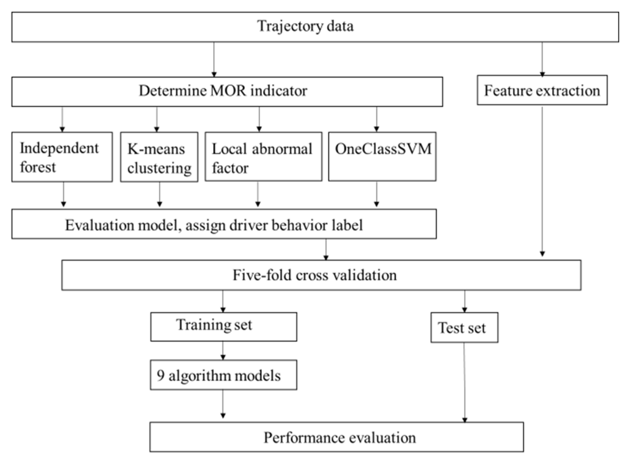
2.2. Classification of Dangerous Driving Behaviors

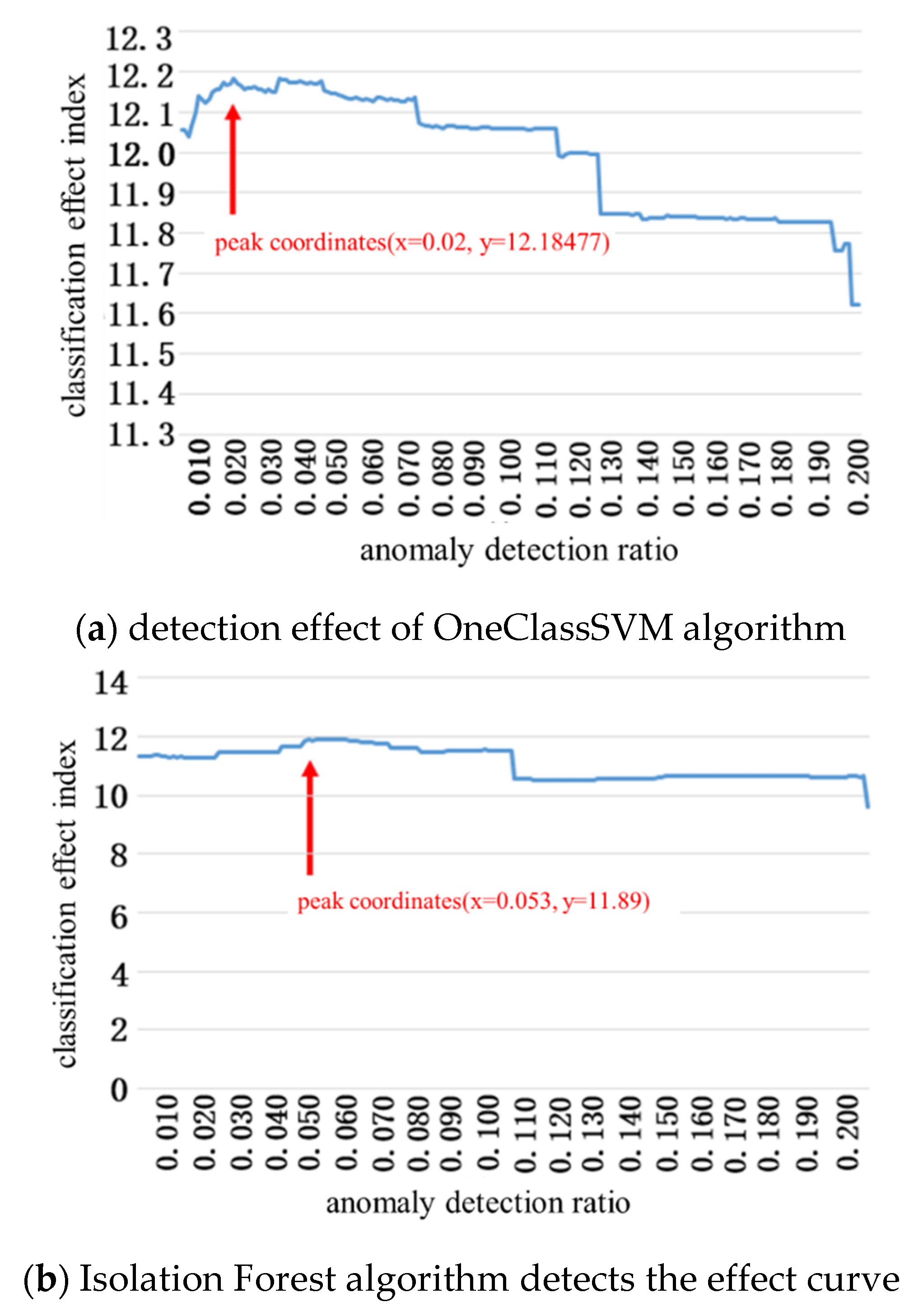
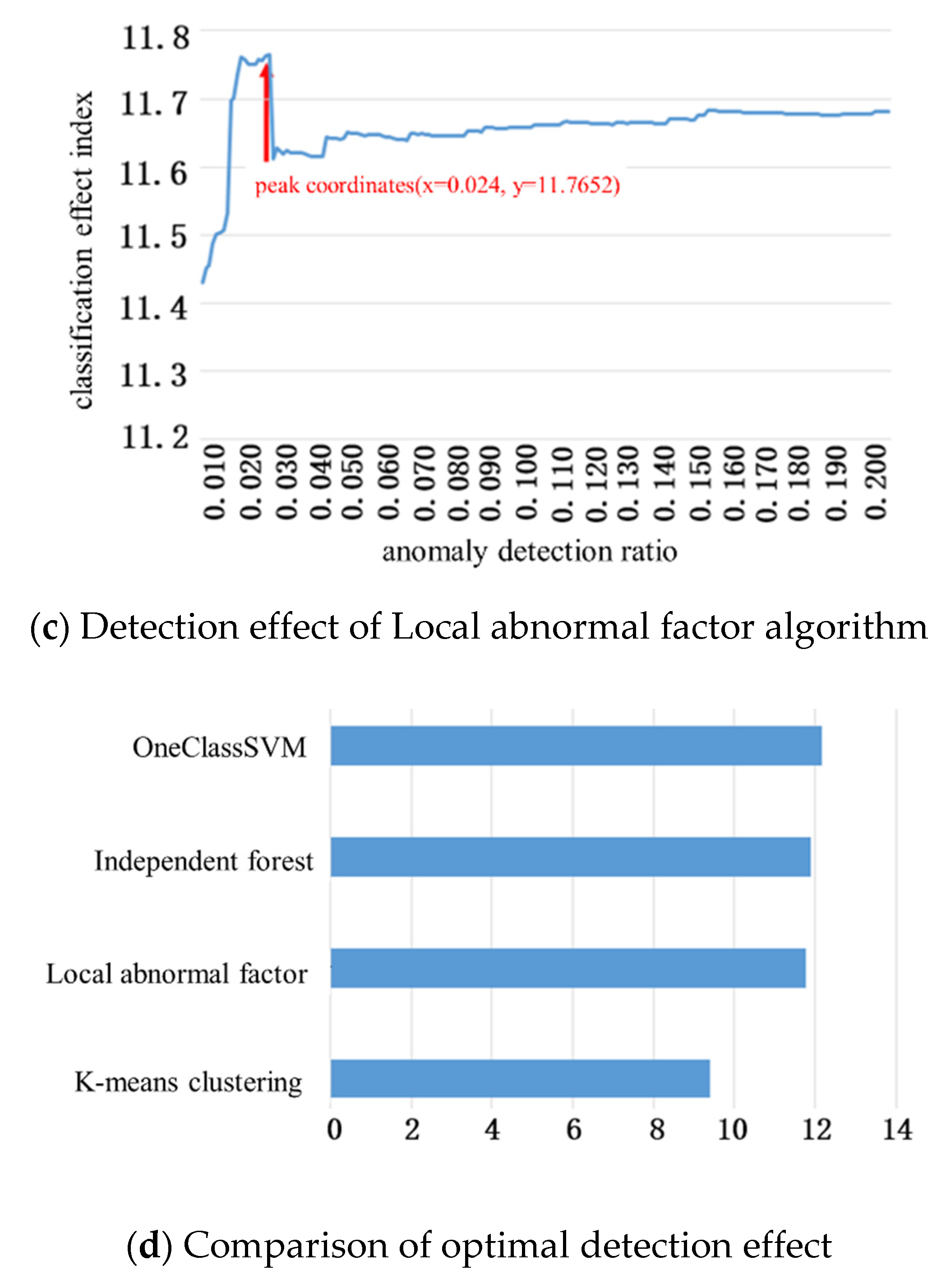
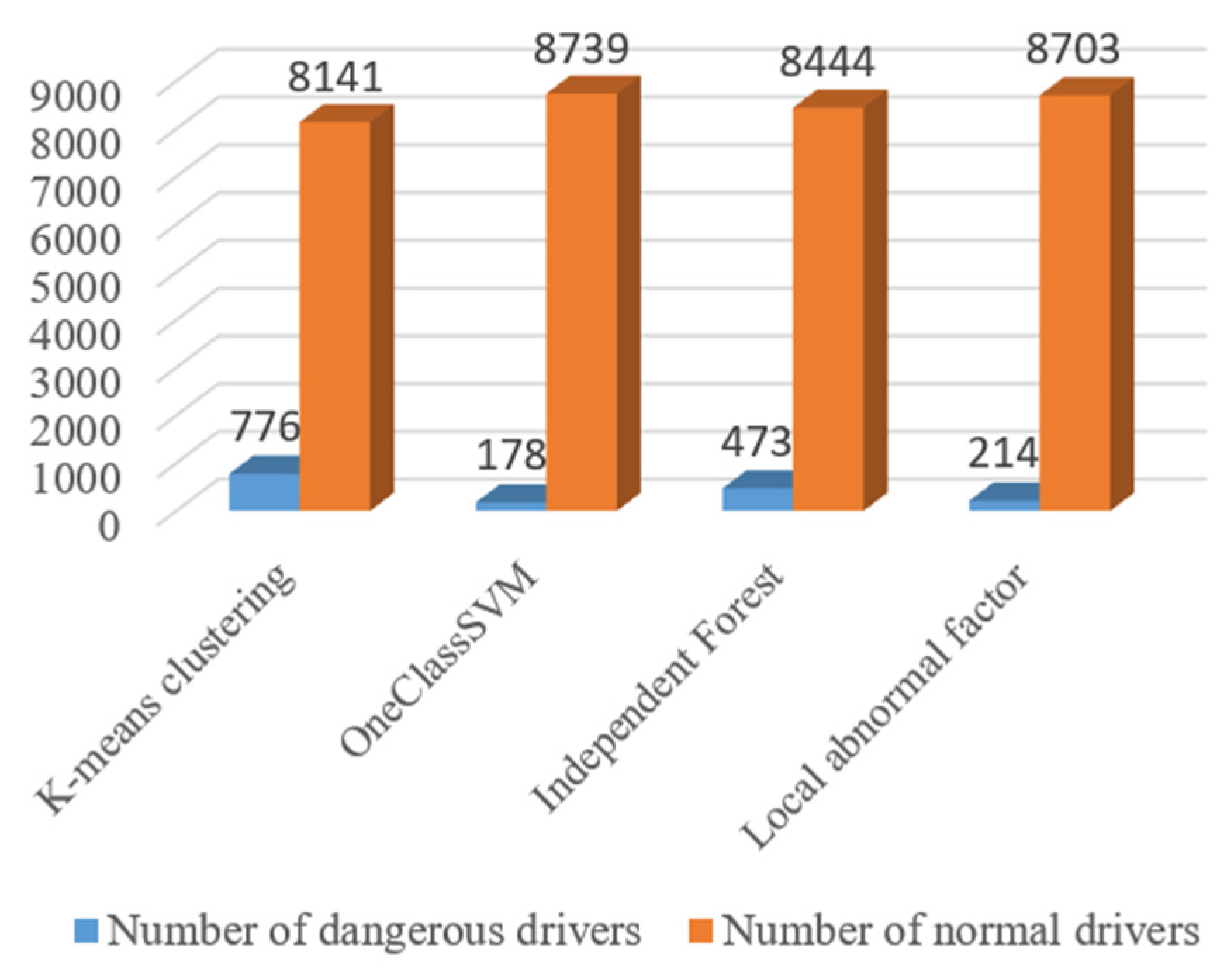
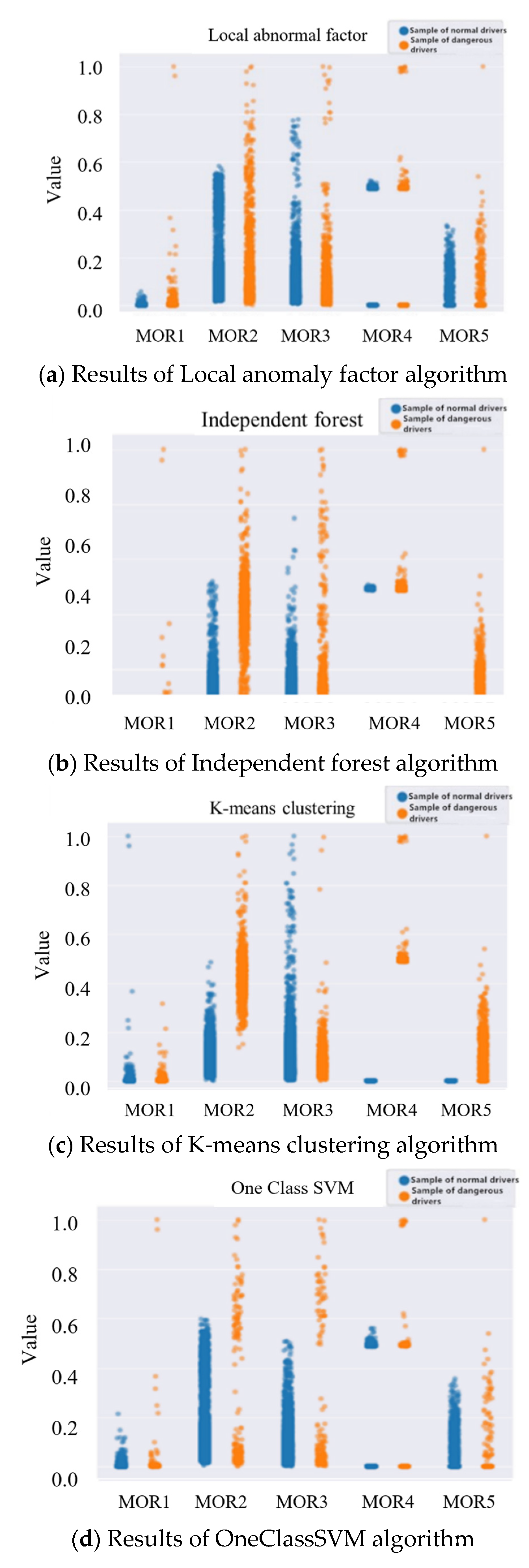
2.2.1. Anomaly Detection Method

Previous studies have shown that the commonly used methods about the determination of threshold values of dangerous driving behavior indicators include statistical methods based on data distribution, clustering methods and abnormal detection methods.

In this paper, four methods including K-means clustering, local factor anomaly algorithm, Isolation Forest and OneClassSVM are employed to analyze dangerous driving behavior. Based on the vehicle’s five dangerous driving behavior characteristics indicators, clustering to find samples with similar data characteristics or outlier abnormal samples by anomaly detection method can distinguish between normal drivers and dangerous drivers.

K-means clustering is a commonly used unsupervised learning method and can be used to identify and detect abnormal points. Given a set of observations (x₁, x₂, ..., x_n), where xi is a d-dimensional real vector. The purpose of K-means clustering is to divide n observations into k clusters {C₁, C₂, ..., C_k} so as to minimize the sum of variance within the cluster. The objective function of K-means clustering is as follows:

$$\mathrm{Min}\mathrm{E}={\displaystyle \sum }_{\mathrm{i}=1}^{\mathrm{k}}{\displaystyle \sum }_{\mathrm{x}\in {\mathrm{C}}_{\mathrm{i}}}{\left|\left|\mathrm{x}-{\mathsf{\mu }}_{\mathrm{i}}\right|\right|}^2$$

(1)

${\mathsf{\mu }}_{\mathrm{i}}=\frac{1}{\left|{\mathrm{C}}_{\mathrm{i}}\right|}{\displaystyle \sum }_{\mathrm{x}\in {\mathrm{C}}_{\mathrm{i}}}\mathrm{x}$ represents the vector mean of the C_i cluster.

Isolation Forest is an efficient anomaly detection algorithm, which has excellent applications in a variety of anomaly detection scenarios. The basic principle is to construct multiple random binary tree subtrees and find outliers by calculating the average path length of the sample to the leaf nodes in all trees. Among them, the abnormal score formula in the independent forest sample is as follows [22]:

$$\mathrm{S}\left(\mathrm{x},\mathsf{\phi }\right)=2^{-\frac{\mathrm{E}\left(\mathrm{h}\left(\mathrm{X}\right)\right)}{\mathrm{c}\left(\mathsf{\phi }\right)}}$$

(2)

E(h(X)) represents the average path length of sample x to the leaf node in multiple subtrees, φ represents the number of training samples of a single binary tree, and c(φ) represents the average path length of training samples. The larger the S value, the more abnormal the data.

The local anomaly factor (LOF) algorithm [23] is also an unsupervised anomaly detection method, which judges abnormal data points by identifying the data points that cross the local density with respect to its neighbors [24]. OneClassSVM is an unsupervised exception detection method [25]. The main implementation principle is to obtain the hypersphere boundary around the data in the feature space by constructing a hypersphere, and to minimize the hypersphere volume as the objective function, so as to identify the outliers.

Suppose the sample training set X = {x₁, x₂, ..., x_n}, ω is a normal vector for the classification hyperplane, v, δ_i is the variable, L is the number of samples, ρ is the constant of the origin relative to the classification surface, φ(x_i) is the mapping function, and the target function is as follows:

$$\min \frac{1}{2}\left||\mathsf{\omega }\right|{|}^2+\frac{1}{\mathrm{vl}}{{\displaystyle \sum }}_{\mathrm{i}=1}^{\mathrm{l}}{\mathsf{\delta }}_{\mathrm{i}}-\mathsf{\rho }$$

(3)

$$\mathrm{s}.\mathrm{t}.·\varnothing \left({\mathrm{x}}_{\mathrm{i}}\right)\ge \mathsf{\rho }-{\mathsf{\delta }}_{\mathrm{i}},{\mathsf{\delta }}_{\mathrm{i}}\ge 0$$

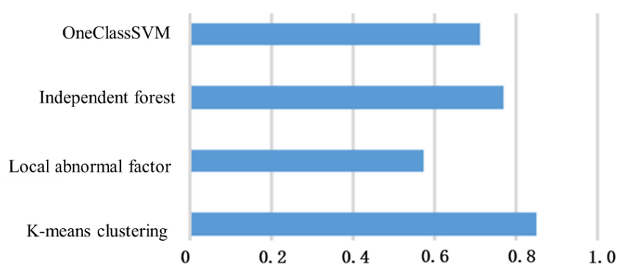
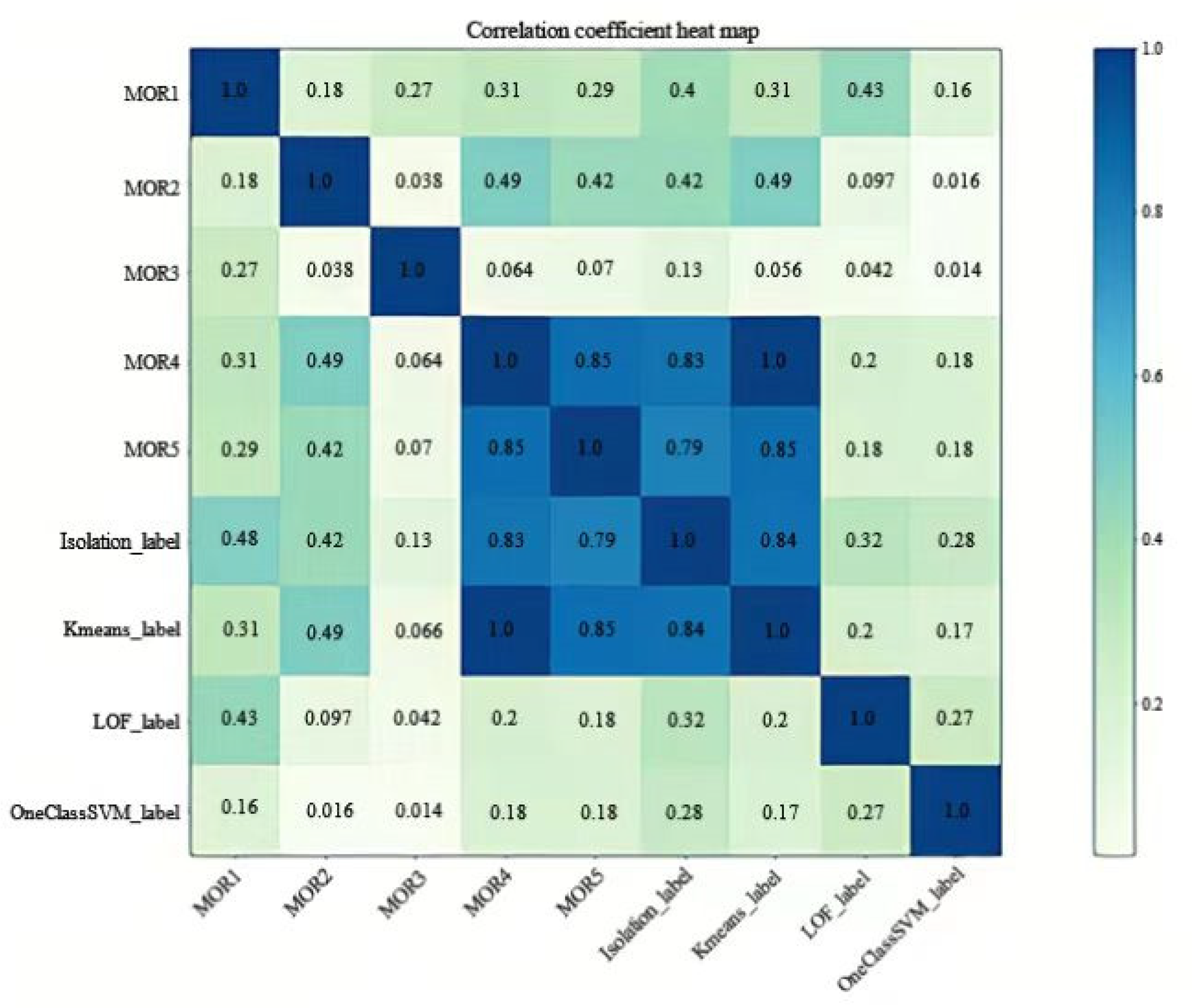
2.2.2. Evaluation of Classification Method

For the evaluation of classification methods, this paper applied contour coefficient, correlation coefficient and category feature analysis methods.

• Contour factor

The contour coefficient is usually used in clustering situations where the actual category information is unknown. For a single sample, suppose a is the average distance from other samples in the same category, and b is the average distance from samples in different categories. The contour coefficient is:

$$\mathrm{S}=\frac{\mathrm{b}-\mathrm{a}}{\max \left(\mathrm{a},\mathrm{b}\right)}$$

(4)

For a sample set, its contour coefficient is the average of the contour coefficients of all samples. The larger the coefficient value, the closer the distance between samples of the same type and the farther the distance between samples of different types.

• Correlation coefficient

This article uses Spearman’s rank correlation coefficient (spearman) to measure the correlation between driving risk index characteristics and driving behavior categories. Assuming that two data vectors in the sample are x (x₁, x₂, ..., x_n), y (y₁, y₂, ..., y_n), the correlation coefficient calculation formula is as follows:

$${\mathsf{\rho }}_{\mathrm{xy}}=\frac{{{\displaystyle \sum }}_{\mathrm{i}}({\mathrm{x}}_{\mathrm{i}}-\tilde{\mathrm{x}})({\mathrm{y}}_{\mathrm{i}}-\tilde{\mathrm{y}})}{\sqrt{{{\displaystyle \sum }}_{\mathrm{i}}{({\mathrm{x}}_{\mathrm{i}}-\tilde{\mathrm{x}})}^2{{\displaystyle \sum }}_{\mathrm{i}}{({\mathrm{y}}_{\mathrm{i}}-\tilde{\mathrm{y}})}^2}}$$

(5)

Among them, when ρ value < 0.05, it is considered that there is a significant correlation between the two vectors. The larger the value of the correlation coefficient ρ_xy, the stronger the correlation, and the positive value of ρ_xy represents the positive correlation between the two vectors.

• Category feature analysis

Unsupervised algorithms usually divide the data into several parts through clustering or anomaly detection, and the evaluation of the algorithm often requires observation of the data characteristics of these parts. Based on the dangerous driving behavior detection scenario, the detection algorithm (including clustering method and abnormal detection method) used in this paper divides the data into normal driving behavior and dangerous driving behavior, and proposes the detection effect index of dangerous driver. Suppose that based on an unsupervised detection algorithm, two driver sample categories are obtained. The normal driver sample is X (x₁, x₂, ..., x_n) and the dangerous driver sample is Y (y₁, y₂, ..., y_m). As shown in Formula (6), the detection effect index of the algorithm consists of the detection effect index of the data in MOR1 to MOR5, and F_ie represents the detection effect index of a certain detection algorithm result in the i-th MOR. As shown in Formula (7), the performance of detection result in the i-th MOR (i = 1, 2, ..., 5) index mainly considers three factors including the normal driver’s maximum MOR feature MOR_ix, the dangerous driver, the distribution shape feature dix and the normal driver distribution shape feature d_iy.

$${\mathrm{F}}_{\mathrm{e}}={{\displaystyle \sum }}_{\mathrm{i}=1}^5{\mathrm{F}}_{\mathrm{ie}}$$

(6)

$${\mathrm{F}}_{\mathrm{ie}}=\{\begin{array}{c}{\mathrm{part}}_{\mathrm{ix}},{\mathrm{MOR}}_{\mathrm{ix}}=0 \\ {\mathrm{K}}_1\ast \mathrm{sig}\left(\frac{1}{{\mathrm{MOR}}_{\mathrm{ix}}}\right)+{\mathrm{part}}_{\mathrm{ix}},{\mathrm{MOR}}_{\mathrm{ix}}\ne 0\end{array}$$

(7)

$${\mathrm{part}}_{\mathrm{ix}}={\mathrm{K}}_3\ast \mathrm{sig}({\mathrm{d}}_{\mathrm{ix}})+{\mathrm{K}}_2\ast \mathrm{sig}({\mathrm{d}}_{\mathrm{iy}})$$

(8)

$$\mathrm{sig}\left(\mathrm{x}\right)=\frac{1}{1+{\mathrm{e}}^{-\mathrm{x}}}$$

(9)

Among them, K₁, K₂, and K₃ are the weight of the maximum MOR characteristics of normal drivers, the distribution characteristics of dangerous drivers, and the distribution characteristics of normal drivers. This research considers the importance of these three to be the same, so this article takes the value k₁ = 1, k₂ = 1, k₃ = 1.

The normal driver’s maximum MOR eigenvalue (MOR_ix) represents the maximum value of the i-th MOR values of the normal driver sample obtained by the detection algorithm. The d_ix represents distribution of normal driver’s MOR value obtained by the detection algorithm in the i-th MOR value range. The specific definition is shown in Formula (10). The d_iy indicates the distribution of the dangerous driver’s MOR value obtained by the detection algorithm in the i-th MOR value range. The specific definition is shown in Formula (11).

$${\mathrm{d}}_{\mathrm{ix}}={{\displaystyle \sum }}_{\mathrm{k}=0.1}^{0.5}\mathrm{N}{\left(\mathrm{i}\right)}_{\mathrm{k}}$$

(10)

$${\mathrm{d}}_{\mathrm{iy}}=\frac{{\mathrm{N}}_{\mathrm{iy}\ge 0.5}}{{\mathrm{N}}_{\mathrm{iy}<0.5}},\mathrm{i}\in \left[1,5\right]$$

(11)

Among them, N_iy ≥ 0.5 represents the number of drivers whose i-th MOR eigenvalue of the dangerous driver sample is greater than 0.5; N_iy < 0.5 represents the drivers whose i-th MOR eigenvalue of the dangerous driver sample is less than 0.5. Assuming xi ∈ X(x₁, x₂, ..., x_n), N(i)_k is defined as shown in Formula (12).

$$\mathrm{N}{\left(\mathrm{i}\right)}_{\mathrm{k}}=\{\begin{array}{c}1 , \exists {\mathrm{x}}_{\mathrm{i}}\in \left[\mathrm{k}-0.1,\mathrm{k}\right) \\ 0 , \nexists {\mathrm{x}}_{\mathrm{i}}\in \left[\mathrm{k}-0.1,\mathrm{k}\right)\end{array}$$

(12)

2.3. Extraction of Characteristics of Driving Behavior

It is all about time series data for driving trajectory data, such as speed, acceleration and so on. The purpose of this research is to identify dangerous driving behaviors by extracting the characteristics of driving trajectory data. In the study of behavior recognition, the methods to obtain the characteristics of time series data mainly include extraction of characteristics in time domain and frequency domain. Because the number of observed frames of each vehicle in the experiment data is inconsistent, the time series of the speed and acceleration of each vehicle cannot be directly used as the input of the recognition model for identifying dangerous driving behavior.

In this paper, the time series of driving characteristics is converted into signal amplitude in the frequency domain, and the first 15 frequency domain components obtained from this characteristic are used as the new characteristic input model.

The DFT of a given time series (x₁, x₂, ..., x_n) is defined as N complex numbers (DFT₀, DFT₁, ..., DFT_N−1):

$${\mathrm{DFT}}_{\mathrm{k}}={\displaystyle \sum }_{\mathrm{n}=0}^{\mathrm{N}-1}{\mathrm{x}}_{\mathrm{n}}{\mathrm{e}}^{\left(-\frac{2\mathsf{\pi }\mathrm{i}}{\mathrm{N}}\mathrm{kn}\right)}$$

(13)

Among them, i is the imaginary unit and e is the base of the natural logarithm.

2.4. Recognition Model

2.4.1. Model Description

Based on the above modeling method, the driver’s driving behavior was labeled and the driving behavior characteristics of each driver were obtained. This section analyzes and compares several recognition models to improve the prediction accuracy. After analyzing the proportion of dangerous driving behaviors, it is found that the driving behavior recognition dataset studied in this paper is extremely imbalanced, so this paper compares multiple imbalanced recognition models for creating optimal algorithm.

All models of dangerous driving behavior recognition employed in this paper are shown in

Table 2. List of recognition models.

Recognition Model	Pretreatment Method	Algorithm Improvement
Adaboost [26,27]	None	None
Rus + Adaboost	Random under-sampling	None
Smote + Adaboost	Smote Oversampling	None
Rusboost [20]	None	Iterative combination Under-sampling
Smoteboost [19]	None	Iterative combination Smote
Xgboost [28]	None	None
Smote + Xgboost	Smote Oversampling	None
Rus + Xgboost	Random under-sampling	None
Imbalance-Xgboost [21]	None	Loss function improvement

, including Adaboost, Smooth + Adboost, Rus + Adaboost, Smoothboost, Rusboost, Xgboost, Smooth + Xgboost, Rus + Xgboost, Imbalance + Xgboost.

Among them, Adaboost and Xgboost are commonly used machine learning algorithms and the driving behavior data are directly recognized without imbalanced processing. “Smote+” means that the data are subjected to the imbalanced processing of the smooth method before training the driving behavior data. “Rus+” means that before using the machine learning model to train the driving behavior data, the data are subjected to the imbalanced processing of the random undersampling method. For example, “Smote + Adaboost” means that during the training of the Adaboost recognition model, the training dataset is processed by the smooth method. The amount of data in each category in the training set is consistent. The Smoteboost and Rusboost are imbalanced boosting algorithms. The standard Adaboost boosting algorithm assigns the same weight to the misclassified samples in each iteration, while the smooth sampling algorithm is used in each iteration in the Smoothboost algorithm to gradually improve the imbalanced ratio of minority samples. In the same way, Rusboost uses a random under-sampling method in each iteration.

To the best of the authors’ knowledge, the imbalance-based improvement of Xgboost in the field of dangerous driving behavior recognition has not been tried (15). The imbalance factor is introduced into the loss function of Xgboost, and the classification effect is adjusted by optimizing the value of the imbalance factor. The entire model can better improve the recognition performance of the minority category that is dangerous driving behavior.

2.4.2. Evaluation Index of Identification Model

For the evaluation of performance of the dangerous driving behavior recognition model, this paper employed four important performance indicators: correct rate, recall rate, F1 value and Auprc value.

The correct rate is defined as follows:

$$\mathrm{precision}=\frac{\mathrm{TP}}{\mathrm{TP}+\mathrm{FP}}$$

(14)

Among them, TP is the number of dangerous drivers who are correctly identified, and FP is the number of normal drivers who are mistakenly identified as dangerous drivers.

The recall rate is defined as follows:

$$\mathrm{Recall}=\frac{\mathrm{TP}}{\mathrm{TP}+\mathrm{FN}}$$

(15)

Among them, FN is the number of dangerous drivers mistakenly identified as normal drivers.

The F1 score is the harmonic average of the correctness rate and the recall rate, where the F1 score reaches the best value at 1 (perfect correctness rate and recall rate) and the worst value at 0. The F1 formula is defined as follows:

$$\mathrm{F}1=\frac{2\ast \mathrm{TP}\ast \mathrm{FN}}{\mathrm{TP}+\mathrm{FN}}$$

(16)

In general, when the observed values of each category are approximately equal, Receiver Operating Characteristic Curve (ROC curve) should be used. When there is imbalanced class, the correct recall rate curve should be used. The ROC curve of an imbalanced dataset may be deceptive and lead to misinterpretation of model performance [29]. Therefore, this research uses the area under the accuracy–recall curve (Auprc) to compare the performance of the algorithm, and calculates the area under the entire accuracy–recall curve as the evaluation index of the performance.

3. Data Description

The dataset is the natural driving vehicle trajectory data token by drones at high altitude on the expressway, and the positioning error is less than 10 cm. The road scene is a two-way four-lane highway, which is a straight road, and in the process of data preprocessing, the paper processes the vehicle trajectory parameters in two directions of the road, respectively. In the video detection process, the length of time that each vehicle is continuously detected and identified is different; that is, the number of frames of each vehicle is not consistent. Therefore, this article first conducts a statistical analysis on the number of frames that all vehicles appear in the video data. In all the collected data, most of the vehicles were identified and observed for more than 10 s (1 s = 10 frames) and the observation frames of the vehicles are basically between 250 and 550. In order to carry out the research on driver’s behavior recognition better, this study mainly focused on the vehicles with the number of observed frames greater than 300 frames. The research objects have a total of 8917 vehicles, including 836 large cars and 8081 small cars.

4. Results

This section may be divided by subheadings. It should provide a concise and precise description of the experimental results, their interpretation, as well as the experimental conclusions that can be drawn.

4.1. Test Results of Dangerous Driving Behavior

The clustering method usually does not impose a mandatory requirement on the number of clustered samples, but the use of anomaly detection algorithm to detect dangerous drivers needs to pre-determine the proportion of dangerous drivers. Based on the abovementioned modeling methods, this paper calculates the performance of an evaluation index of various dangerous driving behavior detection methods to determine the proportion of dangerous driving behavior in the detection algorithm. As shown in the subgraphs a, b, and c of Figure 2, the curves of the detection effects using three algorithms, including OneClassSVM, independent forest and local anomaly factor, under different proportions of dangerous drivers, are obtained. The results show that the classification effect of OneClassSVM is the best when the proportion of dangerous drivers is 0.02. The optimal proportion of dangerous drivers using independent forest is 0.053, and the proportion of optimal drivers using local anomaly factor is 0.024. The Figure 2d shows the optimal detection effect obtained by various detection methods, and the results show that the performance of OneClassSVM for dangerous driving behavior detection is the best.

Various methods for detecting dangerous driving behavior obtain different proportions of dangerous driving behaviors. As shown in Figure 3, the number of dangerous drivers is judged to be the largest based on K-means clustering methods. A total of 776 vehicles are judged as participating in dangerous driving behaviors. The OneClassSVM algorithm shows the least number of dangerous drivers, with a total of 178; the driver’s behavior was judged to be dangerous driving behavior.

Next, this paper uses contour coefficients commonly used in clustering methods to compare various dangerous driver detection methods. As shown in Figure 4, the K-means clustering method shows the largest contour coefficient, followed by independent forest and OneClassSVM. The results show that the contour coefficient obtained by the local anomaly factor is lower than the other three methods, based on the data. This shows that, compared with the local anomaly factor, the distances between samples of dangerous drivers obtained by the other three methods are closer, the distance between samples of dangerous drivers and normal drivers is longer, and the classification performance is relatively better. In addition, the samples of dangerous drivers do not necessarily have similarities in the MOR values, and further correlation analysis of the results and analysis of the MOR distribution of dangerous drivers are needed.

In order to verify the effectiveness of various detection algorithms, this paper uses Spearman’s correlation coefficient to analyze the correlation between category labels and feature variables. Figure 5 shows driving risk indicators (MOR1~MOR5) and the heat map of the correlation coefficient between the labeled data obtained by various detection methods. The legend on the right side of the heatmap shows the color depth, corresponding to different correlation coefficients. The Isolation_label obtained through the independent forest method, kmean_label obtained through the k-means method, LOF_label obtained through the local abnormal factor, and OneClassSVM_label obtained through OneClassSVM.

Among them, the data label is defined as a two-class label, where value 1 represents dangerous driving and value 0 represents normal driving. From the color of the heatmap, the closer it is to white, the weaker the correlation is, and the closer it is to blue, the stronger the correlation is. It can be seen from the figure that the correlation coefficients between the labels obtained by each detection method and the MOR value of the driving risk indicator are all positive, indicating that the greater the degree of driving risk, the more dangerous the driving tends to be, and the lowest correlation is 0.014. It can be seen that all these types of detection methods are effective. From the perspective of the color distribution on the heat map, the correlation between most labels and the mor value of driving risk index is not strong, for example, between MOR3 and the labels by all four algorithms. The data labels obtained by independent forest and k-means clustering have a strong correlation with MOR4 and MOR5, and the data labels obtained by the local anomaly factor and OneClassSVM have a strong correlation with MOR1, but the data labels obtained by local abnormal factor have very weak correlation with MOR1~MOR5. The p-values of all correlation coefficients are less than 0.01.

Finally, this paper compares the data characteristics from the results of two types of samples (normal drivers and dangerous drivers), obtained by various detection methods. Figure 6 shows the data feature distribution map obtained by the four detection methods. As shown in Figure 6a, the blue dots represent samples of normal drivers, and the orange dots represent samples of dangerous drivers. The abscissa represents five driving risk indicators (MOR1~MOR5) and the ordinate represents the value of MOR. Each driving risk indicator on the abscissa corresponds to two columns of distribution maps (normal driving samples and dangerous driving samples). From the abovementioned definition of dangerous driving behavior index, it can be seen that the characteristic of dangerous driving behavior should be that some or all the dangerous driving risk index are relatively large, and the MOR value of the normal driver data sample should be relatively small. Therefore, this research suggests that the range of eigenvalue for dangerous driving behavior is wider than that for normal driving behavior samples. The range of normal driving behavior needs to occupy a certain distribution and cannot be too large.

It can be seen from Figure 6c that, based on the k-means clustering to obtain the classification results, the value ranges of the feature values MOR1 and MOR3 for the normal driver sample points are almost evenly distributed across the entire value range. For drivers, the greater the MOR value, the greater the risk of dangerous driving, and the value of MOR in the normal driver sample obtained by this method is too high. Therefore, this research suggests that this classification method is not practical for identifying dangerous driving behavior. It can be seen from Figure 6b that in the data category of normal drivers obtained by the independent forest algorithm, the feature value of MOR5 is basically 0. Obviously, the classification method mainly refers to whether the lane change insertion feature behavior occurs. The MOR5 feature value is greater than 0, which means that the vehicle has been inserted into lanes. Normal drivers may also have lane-changing insertions. Dangerous driving behaviors should not be classified based on a certain feature. Therefore, the results obtained by this method cannot truly satisfy dangerous driving behavior recognition needs. In Figure 6, the eigenvalue distributions of the algorithm results of sub-Graphs a and d are relatively similar. However, the maximum value of the MOR3 characteristic value of the normal driver in sub-Graph a is higher than that of sub-Graph d. In addition, it can be clearly seen from the sub-Graphs that the eigenvalue range distribution of dangerous driving behavior is wider than that of normal driving behavior, and the MOR eigenvalues of normal driving behavior samples are mainly distributed below 0.6.

Combining the above evaluation methods, this article recommends using OneClassSVM method to calibrate dangerous drivers. This conclusion is consistent with the conclusion obtained from the analysis of the index about detection performance proposed in this paper.

4.2. Results of Dangerous Driving Behavior Recognition

Based on the abovementioned modeling methods, the OneClassSVM abnormality detection is performed on all the vehicle trajectory data to obtain the label of dangerous driver data. After that, the speed and acceleration of each vehicle are subjected to the Fourier transform feature extraction to obtain the parameters of driver behavior characteristics. The results of the comparative analysis of the recognition and classification models are shown in

Table 3. Algorithm performance table.

Algorithm	Correct Rate	Recall Rate	F1	Auprc
Adaboost	0.799	0.597	0.683	0.783
Rus + Adaboost	0.482	0.888	0.624	0.722
Smote + Adaboost	0.544	0.839	0.66	0.758
Rusboost	0.51	0.946	0.663	0.83
Smoteboost	0.531	0.888	0.664	0.791
Xgboost	0.84	0.651	0.733	0.839
Smote + Xgboost	0.621	0.893	0.732	0.811
Rus + Xgboost	0.541	0.918	0.681	0.777
Imblance-Xgboost	0.835	0.691	0.755	0.852

. The recognition process of each recognition model adopts a 5-fold hierarchical cross-validation method. The dataset is divided into five equally. One is selected, in turn, as the test set data, and the remaining four datasets are used as training data. After repeating cross validation five times, the evaluation results based on correctness rate, recall rate, F1 value and Auprc value of the five test set data are averaged to represent the comprehensive recognition performance of the entire algorithm model.

As shown in Table 3, the prediction accuracy of the imbalanced improved Xgboost algorithm is 83.5%, which is only lower than the 84% of Xgboost, indicating that only 16% of the dangerous drivers identified by the model are misjudged. Rusboost has the highest recall rate, which means that 94.6% of dangerous drivers are recognized. The imbalanced improved Xgboost recall rate is higher than that of Xgboost and Adaboost. The data results show that the F1 value and Auprc value obtained by the imbalanced modified Xgboost are the highest. In addition, considering the characteristics of imbalanced processing data, simply preprocessing the data structure through the sampling method cannot significantly improve the recognition performance of the algorithm for identifying dangerous driving behaviors. The other imbalanced promotion algorithm or the methods, including changing the loss function, will be helpful to improve the recognition performance, because the imbalanced promotion algorithm and loss function can change the weight of the model through iterative training and strengthen the learning of the characteristics of minority samples, which is better than the pre-sampling processing method.

5. Conclusions

Based on the real vehicle trajectory data collected based on different highway scenes, this paper defined crash risk indicators of dangerous driving behaviors for five types of driving behaviors, including dangerous car following, lateral deviation, frequent acceleration and deceleration, frequent lane changes, and forced insertion. Through these dangerous driving risk indicators, a variety of methods were employed and compared to detect abnormalities in vehicle trajectory data. An evaluation method for abnormal detection results is proposed to analyze and evaluate the classification results of dangerous drivers. The results show that the data spatial structure of the dangerous driver category obtained by OneClassSVM is more accurate, and the distribution of the MOR range is wider than that of the normal driver. The MOR range of the normal driver category is basically distributed in the low range of 0 to 0.6. Finally, OneClassSVM is used to detect and calibrate dangerous drivers. Aiming at solving the extremely imbalanced characteristics of the dangerous driver dataset, this paper uses a variety of processing methods for comparative analysis. The results show that the improved Xgboost algorithm has the best performance in identifying dangerous drivers, followed by the Xgboost algorithm, and the RusBoost imbalanced lifting algorithm. In summary, this paper proposes an algorithm for detecting dangerous driving behaviors based on vehicle trajectories, which can effectively identify dangerous driving behaviors in advance.

However, in real life, driving behaviors are complex and diverse. In this paper, only mor value is used to identify different driving behaviors. Next, more indicators can be selected for research. In addition, this paper only carries out the identification and analysis of dangerous driving behavior based on video surveillance. In the follow-up research, it can also carry out the research based on on on-board equipment, and conduct in-depth discussion in combination with the two scenes.

References

1. Zhao, L.; Jia, Y. Intelligent transportation system for sustainable environment in smart cities. Int. J. Electr. Eng. Educ. 2021. [Google Scholar] [CrossRef]
2. Borsos, A.; Birth, S.; Vollpracht, H.J. The Role of Human Factors in Road Design. In Proceedings of the IEEE International Conference on Cognitive Infocommunications, Wrocław, Poland, 16–18 October 2016; pp. 363–367. [Google Scholar]
3. Amarasinghe, M.; Muramudalige, S.R.; Kottegoda, S.; Arachchi, A.L.; Muramudalige, S.; Bandara, H.D.; Azeez, A. Cloud-based driver monitoring and vehicle diagnostic with OBD2 telematics. Int. J. Handheld Comput. Res. 2015, 6, 57–74. [Google Scholar] [CrossRef]
4. Wu, M.; Zhang, S.; Dong, Y. A novel model-based driving behavior recognition system using motion sensors. Sensors 2016, 16, 1746. [Google Scholar] [CrossRef] [PubMed] [Green Version]
5. Dula, C.S.; Martin, B.A.; Fox, R.T.; Leonard, R.L. Differing types of cellular phone conversations and dangerous driving. Accid. Anal. Prev. 2011, 43, 187–193. [Google Scholar] [CrossRef]
6. Xu, X. Identification of dangerous driving behaviors based on neural network and Bayesian filter. Adv. Mater. Res. 2013, 846–847, 1343–1346. [Google Scholar] [CrossRef]
7. Chiabaut, N.; Leclercq, L.; Buisson, C. From heterogeneous drivers to macroscopic patterns in congestion. Transp. Res. Part B Methodol. 2010, 44, 308. [Google Scholar] [CrossRef] [Green Version]
8. Hammit, B.E.; Ghasemzadeh, A.; James, R.M.; Ahmed, M.M.; Young, R.K. Evaluation of weather-related freeway car-following behavior using the SHRP2 naturalistic driving study database. Transp. Res. Part F Traffic Psychol. Behav. 2018, 59, 244–259. [Google Scholar] [CrossRef]
9. Xue, Q.W.; Wang, K.; Lu, J.; Liu, Y. Rapid driving style recognition in car-following using machine learning and vehicle trajectory data. J. Adv. Transp. 2019, 2019, 209–219. [Google Scholar] [CrossRef] [Green Version]
10. Agamennoni, G.; Ward, J.R.; Worrall, S.; Nebot, E.M. Anomaly Detection in Driving Behaviour by Road Profiling. In Proceedings of the IEEE Intelligent Vehicles Symposium Workshops, Gold Coast City, Australia, 23–26 June 2013. [Google Scholar]
11. Chen, X.; Xu, X.; Yang, Y.; Wu, H.; Tang, J.; Zhao, J. Augmented ship tracking under occlusion conditions from maritime surveillance videos. IEEE Access 2020, 8, 42884–42897. [Google Scholar] [CrossRef]
12. Chen, X.; Wang, S.; Shi, C.; Wu, H.; Zhao, J.; Fu, J. Robust ship tracking via multi-view learning and sparse representation. J. Navig. 2019, 72, 176–192. [Google Scholar] [CrossRef]
13. Zou, Y.; Lin, B.; Yang, X.; Wu, L.; Muneeb Abid, M.; Tang, J. Application of the Bayesian model averaging in analyzing freeway traffic incident clearance time for emergency management. J. Adv. Transp. 2021, 2021, 6671983. [Google Scholar] [CrossRef]
14. Chen, X.; Chen, H.; Yang, Y.; Wu, H.; Zhang, W.; Zhao, J.; Xiong, Y. Traffic flow prediction by an ensemble framework with data denoising and deep learning model. Phys. A Stat. Mech. Appl. 2021, 565, 125574. [Google Scholar] [CrossRef]
15. Chen, X.; Li, Z.; Yang, Y.; Qi, L.; Ke, R. High-resolution vehicle trajectory extraction and denoising from aerial videos. IEEE Trans. Intell. Transp. Syst. 2020, 22, 3190–3202. [Google Scholar] [CrossRef]
16. Ramyar, S.; Homaifar, A.; Karimoddini, A.; Tunstel, E. Identification of Anomalies in Lane Change Behavior Using One-Class SVM. In Proceedings of the IEEE International Conference on Systems, Budapest, Hungary, 9–12 October 2016. [Google Scholar]
17. Matousek, M.; Yassin, M.; Al-Momani, A.; Heijden, R.; Kargl, F. Robust Detection of Anomalous Driving Behavior. In Proceedings of the 2018 IEEE 87th Vehicular Technology Conference (VTC Spring), Porto, Portugal, 3–6 June 2018; pp. 1–5. [Google Scholar]
18. Chawla, N.V.; Bowyer, K.W.; Hall, L.O.; Kegelmeyer, W.P. SMOTE: Synthetic Minority Over-Sampling Technique. J. Artif. Intell. Res. 2002, 16, 321–357. [Google Scholar] [CrossRef]
19. Chawla, N.V.; Lazarevic, A.; Hall, L.O.; Bowyer, K.W. SMOTEBoost: Improving Prediction of the Minority Class in Boosting. In Proceedings of the Seventh European Conference Principles and Practice of Knowledge Discovery in Databases, Cavtat-Dubrovnik, Croatia, 22–26 September 2003; pp. 107–119. [Google Scholar]
20. Seiffert, C.; Khoshgoftaar, T.; Van Hulse, J.; Napolitano, A. Rusboost: A Hybrid Approach to Alleviating Class Imbalance. In IEEE Transactions on Systems, Man, and Cybernetics-Part A: Systems and Humans; IEEE: New York, NY, USA, 2010; Volume 40, pp. 185–197. [Google Scholar]
21. Chen, T.; Guestrin, C. XGBoost: A Scalable Tree Boosting System. In Proceedings of the 22nd ACM SIGKDD International Conference on Knowledge Discovery and Data Mining, San Francisco, CA, USA, 13–17 August 2016; Volume 1, pp. 785–794. [Google Scholar] [CrossRef] [Green Version]
22. Lin, T.Y.; Goyal, P.; Girshick, R.; He, K.; Dollár, P. Focal loss for dense object detection. IEEE Trans. Pattern Anal. Mach. Intell. 2017, 42, 2999–3007. [Google Scholar]
23. Breunig, M.M.; Kriegel, H.P.; Ng, R.T.; Sander, J. LOF: Identifying density-based local outliers. ACM Sigmod Rec. 2000, 29, 93–104. [Google Scholar] [CrossRef]
24. Liu, F.T.; Ting, K.; Zhou, Z. Isolation-based anomaly detection. ACM Trans. Knowl. Discov. Data 2012, 6, 3. [Google Scholar] [CrossRef]
25. Schölkopf, B.; Platt, J.; Shawe-Taylor, J.; Smola, A.J.; Williamson, R.C. Estimating support of a high-dimensional distribution. Neural Comput. 2001, 13, 1443–1471. [Google Scholar] [CrossRef]
26. Zhu, J.; Zou, H.; Rosset, S.; Hastie, T. Multi-class adaboost. Stat. Terface 2009, 2, 349–360. [Google Scholar]
27. Zhang, J.; Hu, Z.B.; Zhu, X.S. Real-time traffic accident prediction based on Adaboost classifier. J. Comput. Appl. 2017, 37, 284–288. [Google Scholar] [CrossRef]
28. Ma, W.Y.; Chang, R.S. Revision and reliability and validity test of prosocial and aggressive driving behavior scale. Ergonomics 2016, 22, 7–10. [Google Scholar]
29. Saito, T.; Rehmsmeier, M. The precision-recall plot is more informative than the roc plot when evaluating binary classifiers on imbalanced datasets. PLoS ONE 2015, 10, 0118432. [Google Scholar] [CrossRef] [PubMed] [Green Version]
Figure 1. Technical roadmap of Dangerous Driving Behavior Recognition.
Electronics 11 01557 g001
Figure 2. The Diagram of Detection effect analysis.
Electronics 11 01557 g002aElectronics 11 01557 g002b
Figure 3. The ratio of Dangerous drivers.
Electronics 11 01557 g003
Figure 4. Silhouette coefficient.
Electronics 11 01557 g004
Figure 5. The Heat map of Correlation coefficient.
Electronics 11 01557 g005
Figure 6. The distribution of MOR.
Electronics 11 01557 g006