Abstract
Incalculable numbers of patients in hospitals as a result of COVID-19 made the screening of heart patients arduous. Patients who need regular heart monitoring were affected the most. Telecardiology is used for regular remote heart monitoring of such patients. However, the resultant huge electrocardiogram (ECG) data obtained through regular monitoring affects available storage space and transmission bandwidth. These signals can take less space if stored or sent in a compressed form. To recover them at the receiver end, they are decompressed. We have combined telecardiology with automatic ECG arrhythmia classification using CNN and proposed an algorithm named TELecardiology using a Deep Convolution Neural Network (TELDCNN). Discrete cosine transform (DCT), 16-bit quantization, and run length encoding (RLE) were used for compression, and a convolution neural network (CNN) was applied for classification. The database was formed by combining real-time signals (taken from a designed ECG device) with an online database from Physionet. Four kinds of databases were considered and classified. The attained compression ratio was 2.56, and the classification accuracies for compressed and decompressed databases were 0.966 and 0.990, respectively. Comparing the classification performance of compressed and decompressed databases shows that the decompressed signals can classify the arrhythmias more appropriately than their compressed-only form, although at the cost of increased computational time.
1. Introduction
There are many abnormal untimely human deaths due to cardiac arrest. It is the biggest issue that needs to be managed now. The severity of the disease has increased to the extent that not only people from remote areas with limited access to health care utilities are affected, but also people living in urban areas with unhealthy lifestyles [1]. Apart from the mentioned causes, the true motivation of this study is to address the effects of over-flooded hospitals as a result of COVID-19 [2,3,4]. Many studies have shown the effects of COVID-19 on heart patients and vice versa. A heart patient is at the highest risk of infection, and COVID-19 patients are at an elevated risk of heart attacks [5,6]. This makes a real-time ECG acquisition device for sick and quarantined patients of utmost significance [7]. ECG is the most reliable and most straightforward non-invasive technique to determine the pathological condition of the heart. The graphical signals obtained through this consist of a series of peaks and peak intervals, viz. P, Q, R, S, T, and PQ, QRS, ST, etc. A normal ECG signal often termed normal sinus rhythm (NSR) has definite parameters, viz. amplitude and duration preset for each peak and peak intervals, respectively [8]. Changes in any of these fixed values lead to heart arrhythmia. Heart arrhythmia is the change in the heart’s normal rhythm that, if endured, leads to for sudden cardiac death (SCD) [9]. Arrhythmias can be categorized into two types: morphological, i.e., one irregular beat, and rhythmic, i.e., set of irregular rhythms [10].
Our heart is divided into two chambers—atrium and the ventricle. The arrhythmia originating from the atrium chamber is called a supraventricular arrhythmia (SVA) as it is above the ventricle chamber and includes several regular and life-threatening arrhythmias [8]. One critical arrhythmia originating from the atrium is Atrial FIBrillation (AFIB). It can be visually identified through the appearance of some fibrillatory waves instead of P-waves. During AFIB, the heartbeat increases up to 175 bpm, resulting in heart failure and atrial thrombosis [11]. Changes in this chamber disturb heart functioning and alter the conduction process of the ventricle chamber [12]. It is in the ventricle chamber that arrhythmias called ventricular arrhythmias (VA) occur. A patient suffering from ventricular disease often experiences several premature beats before the regular beats. These beats are termed ectopy beats. These beats affect the depolarization process of ventricles and interrupt the blood pumping function. The beats can be either benign or malignant [13]. The malignant heart condition or malignant ventricular ectopy beat (MVE) is fatal as the heart’s contraction may be responsible for SCD, but the benign ectopy beats are not severe. All of these arrhythmias appear alone or in combination. A sample rhythm of all four classes is shown below in Figure 1.
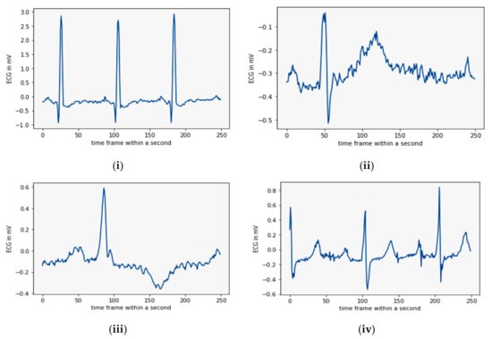
Figure 1.
A set of four sample rhythms: (i) NSR, (ii) AFIB, (iii) MVE, and (iv) SVA (from databases).
By studying several ECG patterns and databases, we have discovered some gaps. Firstly, the appearance of an arrhythmia cannot be tracked by short-time monitoring. Secondly, one arrhythmia can appear in a combination of two or more. Thirdly, the beat-by-beat classification can be replaced by database classification. Fourthly, correct arrhythmia recognition requires a high resolution of the signals [14]. To fill the above gaps here, a longer duration of signal is monitored from the same number of people at different times in a day. The longer signals increase the volume of the data to be transmitted, reducing the transmission efficiency too. The problem is intensified when approx. 300 million ECG recordings need to be sent every year [14]. In this way, a new dilemma of big data handling appears. These big data not only increase desired transmission bandwidth and data rate but also increase the cost of sending it through wired or wireless channels [15]. The literature suggests that the best way to handle this is through compression [16,17]. These signals are compressed at the sending end so that more data can be sent utilizing the available fixed bandwidth and recovered through decompression at the receiver end [18]. Researchers are already working toward finding a good compression scheme and many techniques are already in use [16,17,19,20,21,22,23]. These compression schemes are divided into lossy and lossless techniques. The lossy signals take less space than the losses signals but often distort the signals [16]. These signals lose their medical credibility and mislead the diagnostic process [24]. For this reason, lossless techniques are used for medical signal processing. Lossless compression provides less compression but could retain almost all essential diagnostic information. These schemes are grouped into time domain and frequency domain compression. For telecardiology and automated, computer-aided classification, the time domain features are often affected by the noise present in the physical ECG signals [25]. These noises can be reduced, but the uncertainty present in defining the boundaries of peaks and peak intervals may reduce the usability of these methods [26]. Frequency-domain techniques such as Fourier transform (FT), discrete Fourier transform (DFT), Discrete Cosine Transform (DCT) [27], and discrete wavelet transform (DWT) [9,28,29,30] are used to transform the time domain signals into the frequency domain. The ECG is a non-stationary signal, and FT cannot determine the time of the occurrence of the frequency component [9]. It requires a constant window size to locate all the frequency components, and this can be achieved through short-time Fourier transform (STFT). Appropriate window size selection is quite difficult to address. However, the WT can address the issue more appropriately by choosing a higher or lower window size for the respective frequency signals of non-stationary ECG [31]. The wavelet transforms work upon a suitable selection of mother wavelet according to the signal’s shape, making the process complex.
In addition, WT is a lossy transform. DCT transform provides a lack of discontinuities and keeps the input signal shape intact after transformation. It computes only real coefficients [26]. It is an invertible process. The inverse of DCT, i.e., IDCT, can be applied for inversion of the output usable at the practitioner end. Compression should be designed in a way that it can balance the high compression ratio with the quality of rebuilding of a signal. The DCT coefficients are quantized through the 16 bit quantization method. This method assigns more bits to the significant coefficients and less to the non-significant ones. This improves the resolution of the image. 16 bit quantization is generally used for medical images where retention of diagnostic details is vital. After quantization, the signal coefficients are run length encoded (RLE) and run length decoded (RLD) before IDCT.
Conventionally, Holter monitors are used for this purpose of real-time monitoring but are expensive with an intricate setup to be used in rural scenarios [19]. Replacing this, the rural areas may benefit from the myriad of wearable sensor innovations. For this, the revolutionary Arduino microcontroller-based easy wearable sensors are being designed. They are economical as well as easy to handle even by a novice. An ECG sensor Ad8232 is an excellent choice because it is pre-implemented by various researchers and gives realistic heart signals [32,33,34,35]. The signal obtained from the device can be stored for later processing or sent for real-time monitoring.
The whole telecardiology system is designed based on the requirement of computer-based automatic real-time remote ECG systems [36]. It is expected that such kinds of systems can classify the signals on their own. Classifying different types of arrhythmia into their appropriate cardiac condition is called classification [37].
The conventional classification process includes vigorous manual work, including feature selection and feature extraction through machine learning algorithms [11]. To avoid these shortcomings, the neural network (NN)-based deep learning (DL) can be immensely utilized even for 1-D ECG signals. These models utilize many feature sets by extracting and selecting intrinsic features from neurons on their own. The DLNN (deep learning neural network) method works on layered architecture, and each layer contains a certain number of neurons. Classification accuracy is directly proportional to the number of hidden layers, but comes with the cost of being overburdened by complexity and the computations of the model. Keeping this in mind, the number of hidden layers should be appropriate. Examples of some DL methods are artificial neural networks (ANN) [38], convolution neural networks (CNN) [35,39,40], multilayer perceptron (MLP) [41], long short-term memory (LSTM), deep belief networks (DBN), and recurrent neural networks (RNN) [42]. The usual ANN has only two layers that limit accuracy. In the deep learning ANN, the number of layers was increased for processing. It is based on gradient descent back and forth propagation that adjusts weights. Deep ANN supports parallel processing but has hardware dependency [38]. Even after the compression of signals, real-time devices need more memory to store the data. For this purpose, CNN is recommended to be used on such devices [43]. CNN works in a convolution window to extract the local features of the input signal. This convolution matrix window scans the signal from left to right and top to bottom. This is a non-varying translation, and CNN applies it to other segments through pattern learning [38].
For classification purposes, we performed two experiments—one by classifying compressed data only and the other by classifying decompressed data—to determine whether, during automatic classification, the compressed signals would classify signals efficiently, as decompression of signals increases the time, computation, and complexity of the model. The resultant method with the highest accuracy will be suggested for telecardiology.
This study aims to nurture the area of telecardiology research by analyzing several arrhythmia dataset types to put off SCDs. The process compresses and decompresses the whole database and compares both for classification through a less complex CNN structure. The CNN is feasible for classifying major databases that contain almost all the arrhythmias in real time that can predict the onset of a heart attack. This paper has contributed to various facets of real-time monitoring, which are summarized as follows:
- A real-time ECG signal acquisition device was designed and developed. Additionally, ECG signals were recorded from 18 volunteers. Thus, our database is based on realistic signals.
- Real ECG signals and online ECG signals were combined to form a new database.
- A suitable form of a database for telecardiology was identified using DCT and IDCT in combination through the deep learning classification method CNN.
- The methodology also presents a suitable data augmentation technique for increasing the data points in the database.
The designed algorithm TELDCNN is unique and has the potential use in telecardiology architectures in real-time remote setups. To implement the designed algorithm, this paper is organized as follows: The first section is the introduction; the second section is the methodology of the proposed model that is providing details of the TELDCNN algorithm and divided into subsections; the third section presents the result of the designed methodology; the fourth section presents a comparison of the results with the most prominent findings from the literature; finally, the fifth section concludes the developed algorithm, its findings, and its importance.
2. Materials and Methods
We first started with designing and developing a wearable heart sensor device using Arduino UNO. The obtained real-time signals were compiled with downloaded signals from open-source Physionet datasets on Kaggle’s online python programming environment. An appropriate series of algorithms were planned to achieve the intended outcome. These sequenced algorithms include filtering, compression, decompression, and classification. The process individually classifies the datasets for compressed and decompressed signals using deep CNN methodology. The designed TELDCNN model architecture is well explained in Figure 2. A concise description of each building block of the proposed architecture is given in the following subsections.
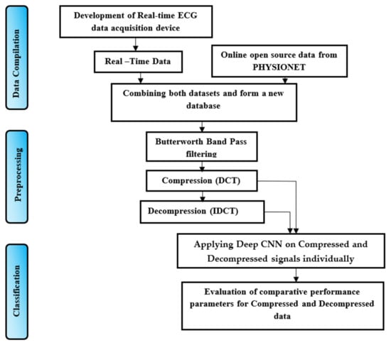
Figure 2.
Processing paradigm for TELDCNN.
2.1. Data Compilation
The data compilation step was added to form a new database that is a combination of both real-time and online databases. The following subsection presents the process of capturing real-time data implemented in this work.
2.1.1. Real-Time Setup
The home health monitoring system was designed using the portable Arduino Uno microcontroller and the ECG sensor chip AD8232. The ECG chip, with three sensor patches and connecting wires, captures the biopotential signals from the skin’s surface. The setup of the proposed work is shown in Figure 3 given below.
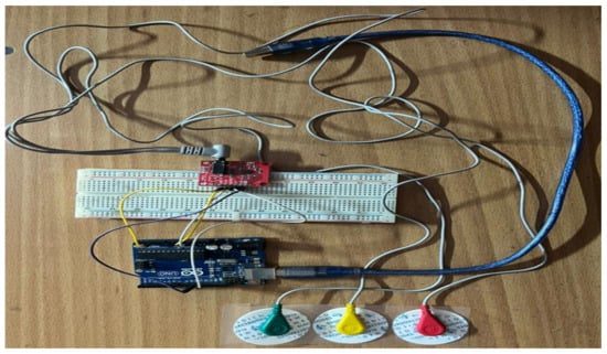
Figure 3.
Overview of our real-time smart wearable ECG acquisition setup.
Arduino UNO (R3) works on an ATmega328-based MCU, with a speed of 16 MHz, a memory of 32 Kb, an operating frequency of170 µA (ultra-low frequency), a common-mode rejection ratio of 80 dB with 100 times amplification factor and filters the signals extracted. The pin-wise connections of Arduino UNO with the ECG sensor board AD8232 is visualized in Figure 4.
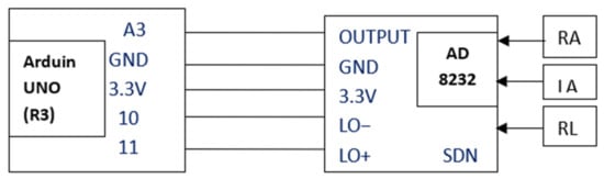
Figure 4.
Pin connection and electrode placement of AD8232.
Figure 4 shows the connections between the Arduino UNO unit and ECG sensor unit AD8232. The connections articulate that the sensor patches attached to the Left Arm LA (yellow wire), Right Arm RA (red wire), and Right Leg RL (green wire) provide heart signals to the AD8232ECG sensor unit [10]. The AD8232 changes the collected heartbeat into an analogue signal. The output is a noisy ECG signal that can be suppressed by the AD8232 Single Lead Heart Rate Monitor. This works similar to an op-amp. This unit has a total of six-pin outings out of which the output is given to A3 of Arduino UNO, GND is connected to GND, 3.3 V connected to 3.3 V, LO− is connected to the pin no. 10 and LO+ to the 11 of Arduino UNO. Another pin SDN of the ECG sensor is left unconnected. The output from Arduino UNO can be visualized on the processing IDE of the serial plotter.
2.1.2. Online Database
For the online database Physionet’s open source, the ECG database was downloaded. Four arrhythmia databases viz. atrial fibrillation, supraventricular, malignant ventricular ectopy beats, and normal sinus rhythms were considered. Specification of each database is given in Table 1 below.

Table 1.
Database specification [44].
MIT-BIH-based ECG databases are the most credible open-source databases available online. They follow the Association for the Advancement of Medical Instrumentation (AAMI) standard for the labeling of the classes.
2.2. Preprocessing
The preprocessing of the ECG signal database comprises filtration and compression. The ECG signals are contaminated through various noises that are due to a number of reasons such as contraction of muscles or movement of electrodes. Baseline wander, and power-line interference are types of noise; of which, baseline wander is placed under low-frequency noise and is related to baseline displacement. There are also high- or low-frequency types. A combination of high- and low-pass filters is required to remove both kinds of noise. The Butterworth bandpass filter (BBF) provides both, i.e., HPF (at 1 Hz) and LPF (at 30 Hz), and improves the quality of the signal. A third-order BBF was used, which can be mathematically defined by the following equation.
where n is the filter order, is the angular gain and is the cut-off frequency. is the maximum passband gain. Its value is 1 at −3dB corner point cutoff. Otherwise, it can be calculated by the relation H1 = , where H0 is the maximum pass band and H1 is the minimum pass band gain. The process gives a de-noised real-time signal illustrated in the results section.
A lossy compression codec methodology is applied to accomplish preprocessing of the ECG signals after filtering, which is a combination of DCT, quantization, run length encoding, run length decoding and IDCT. Figure 5 explains the compression codec process.
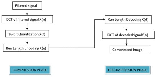
Figure 5.
Compression codec of TELDCNN.
DCT is a lossless, frequency domain-based predesigned compression algorithm that has already been applied by many studies and performs remarkably. It is an orthogonal Fourier transform-based technique that uses only positive components and can reduce redundancy with its transform coefficients containing most signal information. It divides the signal into N no. of subparts and computes DCT on them. After DCT computation, thresholding and quantization of the transform coefficients are performed. The mathematical representation of DCT can be explained through Equations (2) and (3):
In the process, the ECG signal is divided into the non-overlapping blocks of size 8 × 8. The basis of the ECG signals changes by computing the DCT of each block. To reduce the size of the image, further quantization of the DCT coefficients is performed. Quantization is the process of slicing the amplitude or intensity of the signal into the discrete level. To retain the diagnostic details of the signal and to improve the resolution, a 16 bit quantization was used. The idea behind this is to allocate more bits to the important coefficients. For this purpose, a threshold value was used. The calculation of the threshold value was performed through the following steps:
X(f) is the quantized DCT signal coefficient.
After quantization, lossless run length encoding of quantized DCT coefficients was performed. X(f) is the input to the encoder. The encoding process was followed by the decoding process applying the same phenomenon. The output of the decoded signal was taken as X(d).
In the decompression phase, the inverse of DCT, i.e., IDCT, is applied and it is given by
where .
For IDCT, X(d) coefficients is the input, transforming them into f(n) back.
After this stage, we obtained two databases, i.e., a compressed signals database and a decompressed signals database. These two databases contain four classes of arrhythmic datasets. The compressed and decompressed outputs are illustrated in the results section.
2.3. Data Augmentation
A high volume of training data is required for classification through deep learning algorithms. In the process of making the length of each database equal by reducing the number of signals in each class and creating them equal to the signal having the lowest length, the total available data volume was reduced. The data augmentation technique can be used to increase the data points to be accessed for classification. Table 2 shows below the duration of data before and after augmentation from each database class.
Table 2.
Illustration of data augmentation outcomes.
The augmentation increases data artificially by up to 6-fold the original by generating new data points [45] and reduces overfitting during classification. In the proposed work, a sliding window technique was implemented that takes one-third of the previous recording and remains from the following sample. In this work, the total duration of the original data was 4320 s, and it becomes 14,122 s, i.e., more than 3-fold the original duration. This whole database can now be finally divided into training, test, and validation signals for classification.
2.4. CNN Structure and Parameter Detail
This section is regarding the elaboration of the deep CNN structure implied for the proposed work. CNN mainly uses two operations, i.e., convolution and pooling, to reduce the input image into its crucial features. These features are used for the classification of input images into different classes. It is mostly made up of convolution, pooling, and fully connected layers. First, a mask is created that moves through the input, and the corresponding mask filter elements or weights are multiplied with the input pixels and sum up the products. The process is repeated until all the values of an image are calculated. Table 3 shows the layer-by-layer description of applied CNN.
Table 3.
Designed CNN sequential model structure.
Table 3 above shows a two-layer CNN structure, where each layer consists of a convolution, batch normalization and max pooling layer, respectively. Here, kernel size was taken as 5, which is the size of the filter used for the input image and stride size was taken as 3. With this size of the stride, the filter was advanced by three pixels at each step of sliding over the input image and divides the image into fewer steps. The larger stride sizes down sample the image quality. The batch normalization layer is used to reduce the internal covariate shift of the network and works on mini-batches [45]. The max-pooling layer used to generate new feature maps by taking the maximum values in the prescribed region on the feature map attained from the last layer hence reduces the dimension again [9]. The output from the first convolution layer is [none, 82, 64], whereas the output image size of the second convolution layer is [none, 13, 64]. The output image size represents the batch size, height, and width, respectively. The two-layer CNN structure is connected with the flattened layer through a dropout layer. The dropout layer here is inserted to reduce overfitting, and the flattened layer is inserted to change the output into a single column matrix. The resultant features from the flattened layer are fed to a dense-connected neural network layer of [512] nodes. Then, a dropout layer is again added.
By using the dropout technique, the random samples of the activations are made zero and deleted. This makes the network only learn the features that increase classification accuracy [9]. Finally, the last dense layer shows the number of output classes required. The sigmoid function was used to predict the class to which the input test data belong. Loss calculation was performed through categorical cross-entropy, and the adaptive moment (ADAM) optimizer was implied. The ADAM optimizer is used for back propagation. It only updates weights based on value and gradient during CNN training [46]. A total of 100 epochs were used during network training, and network weights were updated during each epoch.
2.5. Performance Parameter Used
To determine the effectiveness of the designed algorithm, the proposed work utilizes performance metrics such as MSE, PSNR, CR, accuracy, sensitivity, F-measure, and precision. The formula for calculating all of these is given by Equations (4)–(11).
- Peak Signal-To-Noise Ratio (PSNR) is used to compare image compression quality. Mean Square Error (MSE) will be calculated. MSE is the cumulative squared error between the compressed and the original image, which can be given by
PSNR is the ratio of signal power to noise power and is given using the value of MSE, expressed in dB.
- 2.
- The compression ratio (CR) is defined as the ratio of the number of bits required to show an image before compression to the bits required after compression.
- 3.
- Accuracy is defined as the ratio of the number of correctly classified cases.
- 4.
- Sensitivity is also called recall. It gives the fraction of correctly predicted positive samples out of the true-positive and false-negative samples within the class. It is a true-positive rate [47].
- 5.
- Specificity is defined as the capability of the model to calculate true-negative values correctly identified within the class. It determines the number of true-negative-labeled beats identified by the model.
- 6.
- F—measure—calculates the recall and precision metrics balance. It is beneficialto use this in the case of imbalanced classes.
- 7.
- Precision is a measure of positive predictivity. It gives a ratio of the true positive observations, and the total predicted positive samples. Higher values indicate a low false-positive rate.
3. Results
In this section, we present the outcomes from each building block described in the proposed work’s opted methodology. According to the method, the foremost task is gathering volunteers’ real-time signals. For this purpose, the design of the device has already been discussed. Now, the following sub-section illustrates the real-time sample outputs.
3.1. Real-Time ECG Signals
The real-time signals taken from the designed setup consist of 1 min-long ECG rhythms (from 18 volunteers). These people were in the age group of 24–47 years. All the received signals have shown normal heart rhythm. A 780s long database was obtained. The CSV file of each of the volunteers shows some 15,000 samples that include high-frequency noise peaks also. The ECG graph plotted by readings shows 55 to 110 cycles per minute. That means all the signals come under NSR. Figure 6 illustrates signal no.1 and signal no.2 out of 18 signal files for 200 samples that make approximately one ECG signal cycle. Similarly, Figure 6 shows 15,000 samples of signals 1 and 2.
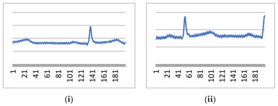
Figure 6.
First 200 samples from (i) signal 1 and (ii) signal 2.
It is evident from the above figures that our designed real-time device is working perfectly and capturing ECG signals which the clinician also verifies. However, these signals are contaminated through high-frequency and low-frequency noise, as visualized in Figure 6 and Figure 7. Both noises can be cleaned through the pre-explained Butterworth bandpass filtering in the following sub-section.
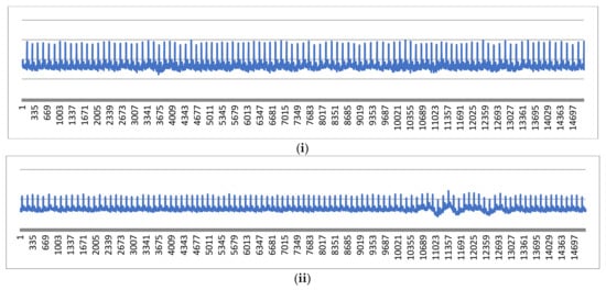
Figure 7.
First 15,000 samples from (i) signal 1 and (ii) signal 2.
3.2. Filtered Signal Output
The filtered output of the applied BBF on the real-time ECG signal and its raw input signal can be illustrated in Figure 8.
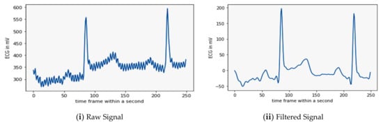
Figure 8.
Illustration of sample raw and filtered signal from real-time database.
Figure 8ii is the sample output signal of the BBF. It shows that the BBF can eliminate both high and low-frequency noise and make the valuable signal for further processing and classification. The next step in the processing of the filtered signal is its compression; the results of which are elaborated in the following sub-section.
3.3. Compression andDecompression Outcomes
After filtering, a series of operations viz. DCT, 16 bit quantization, run length encoding, and run length decoding were applied to reduce the size of the signals. The compressed form of the signals is sent to the receiver end, where the signals are decompressed by IDCT. Here, we have shown in Figure 9 the DCT, quantized and IDCT sample signals from the filtered data of the last stage.
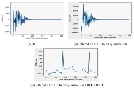
Figure 9.
Sample signal representation of compressed and decompressed signals.
While comparing the output of Figure 8, i.e., the noiseless input signal of the DCT with the final output of the IDCT, the visual difference between both the signals is significantly less. Hence, the implied compression has not deteriorated the quality of the signal and can be used for classification. A detailed explanation of both the techniques was given in Section 2.2, i.e., ‘Preprocessing’.
By applying a 16 bit quantization on the DCT coefficients, the PSNR becomes 43.6 dB, while the CR value obtained was 1:2.56.
3.4. Final Classification Result
The performance of the proposed algorithm was determined based on the ECG database created through signals taken from real-time devices and the Physionet. All the signals were re-sampled at a 250 Hz sampling frequency. The real-time signals are mostly normal sinus rhythms added with the NSR Physionet database. All the databases are compressed through DCT and then decompressed through IDCT. Now two new databases were created, i.e., compressed and decompressed. A similar deep CNN classification algorithm was applied on both individually. To evaluate the classification performance of the designed CNN, both databases will be evaluated separately and then compare based on performance factors. A confusion matrix for both compressed and decompressed databases, respectively, is drawn in Figure 10.
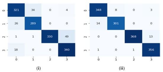
Figure 10.
Confusion matrixes for (i) the compressed database and (ii) the decompressed database.
Using the above confusion matrix, parameters such as true positive (TP), true negative (TN), false positive (FP), and false negative (FN) can be calculated, which are Tp = 321, FP = 45, FN = 38 and TN = 1009 for the compressed signal database and for the decompressed signal database Tp = 348, FP = 15, FN = 11 and TN = 1026. The performance factors of the database classification method were estimated based on these values. Table 4, shown below, explains this using numeric values.
Table 4.
Classification performance of the compressed signal and the decompressed signal database.
Consequently, Table 4 elaborates on the finding attained after the deep CNN was applied to the compressed and decompressed signals. It shows 96.6% accuracy and 99% accuracy, respectively. This indicates that the decompressed signals performed better during telecardiology and classified the databases efficiently.
4. Discussion
It is clear from the above results that a deep CNN gives the highest possibility of classifying the arrhythmia data class in the right cluster when applied to the decompressed signal database. Table 5 shows the importance of the work in comparison to many existing recent algorithms.
Table 5.
Comparison of TELDCNN with other state-of-the-art algorithms.
The Q-wavelet-based method in [9] has less CR with less accuracy and sensitivity of classification through machine learning-based algorithm SVM. The machine learning-based algorithms are lengthy and not automatic as they depend upon manual ECG feature extraction and selection process. A random forest-based classification was performed in [23] for the signals compressed through the 1 bit quantization compression technique. It attained 0.94 accuracy, which is lower than our compressed classification output. Similarly, other methods such as MOWPT compression, FDResNet, 2D-CNN, multiple measurement vector (MMV) were accessed to compare the results obtained through the designed algorithm.
This shows that the designed TELDCNN algorithm is unique and supportive in developing telecardiology.
5. Conclusions
The methodology was designed to benefit the many people who cannot access expensive health care services and are in remote areas. This makes the telecardiology system prompt and efficient. To realize this system, ECG acquisition and processing techniques are combined with the goal of arrhythmia recognition. The designed system includes a low-power and a low-cost handheld ECG recording device. The developed device helped to take real-time signals from volunteers. A combination of open-source and real-time databases are used to determine the classification performance of compressed and decompressed signals. For compression DCT, 16 bit quantization, RLE, decompression, and IDCT were applied, resulting in a compression ratio of 2.56. The algorithm compares the classification performance for both. It was evident from the results that the designed CNN structure classifies the decompressed signal dataset with 99% and the compressed set with 96.6% accuracy. Though the computation in the later dataset is lower, the prior performance is higher. Telecardiology requires reducing the redundant data present in the dataset to improve the efficiency of real-time devices. It also decreases the required power, bandwidth, storage, etc. Hence, we have obtained a TELDCNN algorithm for automatically classifying decompressed data. In the future, this work will be extended by introducing cloud computing for telecardiology. In future works, other mobile methodologies which aggregate monitoring and mapping of the environment will be performed using Wall-Following, Simultaneous Location and Mapping (SLAM) and Sensor Fusion techniques and can be applied to the problem in question [55].
Author Contributions
Conceptualization E.S. and A.N.; methodology E.S.; software P.G. and E.S.; validation, P.G.; formal analysis E.S. and A.N.; investigation P.R.P.; resources E.S.; data curation, E.S. and P.R.P.; writing—E.S.; writing—review and editing E.S., P.R.P. and P.G.; visualization A.N. and P.G.; supervision, A.N. and P.R.P.; project administration, P.R.P.; funding acquisition, P.R.P. All authors have read and agreed to the published version of the manuscript.
Funding
This research received no external funding.
Informed Consent Statement
Written informed consent has been obtained from the patients to publish this paper.
Data Availability Statement
https://www.kaggle.com/datasets/ektasoni/ecg-data-set (accessed on 2 August 2022).
Acknowledgments
P.R.P. is grateful to the University of Fortaleza / Edson Queiroz Foundation and to the National Council for Scientific and Technological Development (CNPq) for developing this project.
Conflicts of Interest
The authors declare no conflict of interest.
References
- Hua, J.; Xu, Y.; Tang, J.; Liu, J.; Zhang, J. ECG heartbeat classification in compressive domain for wearable devices. J. Syst. Arch. 2019, 104, 101687. [Google Scholar] [CrossRef] [PubMed]
- Rincon, J.A.; Guerra-Ojeda, S.; Carrascosa, C.; Julian, V. An IoT and Fog Computing-Based Monitoring System for Cardiovascular Patients with Automatic ECG Classification Using Deep Neural Networks. Sensors 2020, 20, 7353. [Google Scholar] [CrossRef]
- CDC COVID-19 Response Team; Bialek, S.; Boundy, E.; Bowen, V.; Chow, N.; Cohn, A.; Dowling, N.; Ellington, S.; Gierke, R.; Hall, A.; et al. Severe outcomes among patients with coronavirus disease 2019 (COVID-19)—United States, February 12–March 16, 2020. Morb. Mortal. Wkly. Rep. 2020, 69, 343. [Google Scholar]
- Adans-Dester, C.; Bamberg, S.; Bertacchi, F.; Caulfield, B.; Chappie, K.; Demarchi, D.; Erb, M.K.; Estrada, J.; Fabara, E.E.; Freni, M.; et al. Can mHealth Technology Help Mitigate the Effects of the COVID-19 Pandemic? IEEE Open J. Eng. Med. Biol. 2020, 1, 243–248. [Google Scholar] [CrossRef] [PubMed]
- Ji, N.; Xiang, T.; Bonato, P.; Lovell, N.H.; Ooi, S.Y.; Clifton, D.A.; Akay, M.; Ding, X.R.; Yan, B.P.; Mok, V.; et al. Recommendation to use wearable-based mhealth in closed-loop management of acute cardiovascular disease patients during the COVID-19 pan-demic. IEEE J. Biomed. Health Inform. 2021, 25, 903–908. [Google Scholar] [CrossRef]
- Nishiga, M.; Wang, D.W.; Han, Y.; Lewis, D.B.; Wu, J.C. COVID-19 and cardiovascular disease: From basic mechanisms to clinical perspectives. Nat. Rev. Cardiol. 2020, 17, 543–558. [Google Scholar] [CrossRef]
- Emokpae, L.E.; Emokpae, R.N.; Lalouani, W.; Younis, M. Smart multimodal telehealth-IoT system for COVID-19 patients. IEEE Pervasive Comput. 2021, 20, 73–80. [Google Scholar] [CrossRef]
- DeSimone, C.V.; Naksuk, N.; Asirvatham, S.J. Supraventricular arrhythmias: Clinical framework and common scenarios for the internist. Mayo Clin. Proc. 2018, 93, 1825–1841. [Google Scholar] [CrossRef]
- Chowdhury, M.; Poudel, K.; Hu, Y. Compression, Denoising and Classification of ECG Signals using the Discrete Wavelet Transform and Deep Convolutional Neural Networks. In Proceedings of the 2020 IEEE Signal Processing in Medicine and Biology Symposium (SPMB), Philadelphia, PA, USA, 5 December 2020; IEEE: Philadelphia, PA, USA, 2020; pp. 1–4. [Google Scholar] [CrossRef]
- Luz, E.J.D.S.; Schwartz, W.R.; Cámara-Chávez, G.; Menotti, D. ECG-based heartbeat classification for ar-rhythmia detection: A survey. Comput. Methods Programs Biomed. 2016, 127, 144–164. [Google Scholar] [CrossRef]
- Da Poian, G.; Liu, C.; Bernardini, R.; Rinaldo, R.; Clifford, G. Atrial fibrillation detection on compressed sensed ECG. Physiol. Meas. 2017, 38, 1405–1425. [Google Scholar] [CrossRef]
- Simanjuntak, J.E.S.; Khodra, M.L.; Manullang, M.C.T. Design methods of detecting atrial fibrillation using the recurrent neural network algorithm on the Arduino AD8232 ECG module. IOP Conf. Ser. Earth Environ. Sci. 2020, 537, 012022. [Google Scholar] [CrossRef]
- Gawde, P.R.; Bansal, A.K.; Nielson, J.A. Integrating Markov model and morphology analysis for real-time finer ventricular arrhythmia classification. In Proceedings of the 2017 IEEE EMBS International Conference on Biomedical & Health Informatics (BHI), Orlando, FL, USA, 16–19 February 2017; pp. 409–412. [Google Scholar]
- Tutuko, B.; Nurmaini, S.; Tondas, A.E.; Rachmatullah, M.N.; Darmawahyuni, A.; Esafri, R.; Firdaus, F.; Sapitri, A.I. AFibNet: An implementation of atrial fibrillation detection with convolutional neural network. BMC Med. Inform. Decis. Mak. 2021, 21, 21. [Google Scholar] [CrossRef]
- Kumar, R.; Kumar, A.; Singh, G.; Lee, H. Efficient compression technique based on temporal modelling of ECG signal using principle component analysis. IET Sci. Meas. Technol. 2017, 11, 346–353. [Google Scholar] [CrossRef]
- Jha, C.K.; Kolekar, M.H. Tunable Q-wavelet based ECG data compression with validation using cardiac ar-rhythmia patterns. Biomed. Signal Processing Control. 2021, 66, 102464. [Google Scholar] [CrossRef]
- Singh, A.; Dandapat, S. Exploiting multi-scale signal information in joint compressed sensing recovery of mul-ti-channel ECG signals. Biomed. Signal Processing Control. 2016, 29, 53–66. [Google Scholar] [CrossRef]
- Rebollo-Neira, L. Effective high compression of ECG signals at low level distortion. Sci. Rep. 2019, 9, 4564. [Google Scholar] [CrossRef]
- Kohno, R.; Abe, H.; Benditt, D.G. Ambulatory electrocardiogram monitoring devices for evaluating transient loss of consciousness or other related symptoms. J. Arrhythmia 2017, 33, 583–589. [Google Scholar] [CrossRef]
- Cheng, Y.; Ye, Y.; Hou, M.; He, W.; Pan, T. Multi-label arrhythmia classification from fixed-length com-pressed ECG segments in real-time wearable ECG monitoring. In Proceedings of the 2020 42nd Annual International Conference of the IEEE Engineering in Medicine & Biology Society (EMBC), Montreal, QC, Canada, 20–24 July 2020; pp. 580–583. [Google Scholar]
- Zhang, H.; Dong, Z.; Wang, Z.; Guo, L.; Wang, Z. CSNet: A deep learning approach for ECG compressed sensing. Biomed. Signal Process. Control 2021, 70, 103065. [Google Scholar] [CrossRef]
- Qaisar, S.M.; Subasi, A. Cloud-based ECG monitoring using event-driven ECG acquisition and machine learning techniques. Phys. Eng. Sci. Med. 2020, 43, 623–634. [Google Scholar] [CrossRef]
- Atal, D.K.; Singh, M. A dictionary matrix generation based compression and bitwise embedding mechanisms for ECG signal classification. Multimed. Tools Appl. 2020, 79, 13139–13159. [Google Scholar] [CrossRef]
- Němcová, A.; Vítek, M.; Maršánová, L.; Smíšek, R.; Smital, L. Assessment of ECG signal quality after com-pression. In World Congress on Medical Physics and Biomedical Engineering 2018; Springer: Singapore, 2019. [Google Scholar]
- Polanía, L.F.; Plaza, R.I. Compressed sensing ECG using restricted Boltzmann machines. Biomed. Signal Process. Control 2018, 45, 237–245. [Google Scholar] [CrossRef]
- Raj, S.; Ray, K.C. ECG Signal Analysis Using DCT-Based DOST and PSO Optimized SVM. IEEE Trans. Instrum. Meas. 2017, 66, 470–478. [Google Scholar] [CrossRef]
- Abdulbaqi, A.; Abdulhameed, A.; Obaid, A. A secure ECG signal transmission for heart disease diagno-sis. Int. J. Nonlinear Anal. Appl. 2021, 12, 1353–1370. [Google Scholar]
- Bera, P.; Gupta, R.; Saha, J. Preserving Abnormal Beat Morphology in Long-Term ECG Recording: An Efficient Hybrid Compression Approach. IEEE Trans. Instrum. Meas. 2019, 69, 2084–2092. [Google Scholar] [CrossRef]
- Chandra, S.; Sharma, A.; Singh, G.K. A Comparative Analysis of Performance of Several Wavelet Based ECG Data Compression Methodologies. IRBM 2020, 42, 227–244. [Google Scholar] [CrossRef]
- Raeiatibanadkooki, M.; Quchani, S.R.; KhalilZade, M.; Bahaadinbeigy, K. Compression and encryption of ECG signal using wavelet and chaotically Huffman code in telemedicine application. J. Med. Syst. 2016, 40, 73. [Google Scholar] [CrossRef]
- Wasimuddin, M.; Elleithy, K.; Abuzneid, A.; Faezipour, M.; Abuzaghleh, O. Multiclass ECG signal analysis using global average-based 2-D convolutional neural network modeling. Electronics 2021, 10, 170. [Google Scholar] [CrossRef]
- Ghifari, A.F.; Perdana, R.S. (2020). In Minimum System Design of the IoT-Based ECG Monitoring. In Proceedings of the 2020 International Con-ference on ICT for Smart Society (ICISS), Bandung, Indonesia, 19–20 November 2020. [Google Scholar] [CrossRef]
- Kanani, P.; Padole, M. Recognizing Real Time ECG Anomalies Using Arduino, AD8232 and Java. In International Conference on Advances in Computing and Data Sciences; Springer: Singapore, 2018; pp. 54–64. [Google Scholar] [CrossRef]
- Bravo-Zanoguera, M.; Cuevas-González, D.; García-Vázquez, J.P.; Avitia, R.L.; Reyna, M.A. Portable ECG System Design Using the AD8232 Microchip and Open-Source Platform. Proceedings 2019, 42, 49. [Google Scholar] [CrossRef]
- Niu, J.; Tang, Y.; Sun, Z.; Zhang, W. Inter-Patient ECG Classification with Symbolic Representations and Multi-Perspective Convolutional Neural Networks. IEEE J. Biomed. Health Inform. 2019, 24, 1321–1332. [Google Scholar] [CrossRef]
- Anker, S.D.; Koehler, F.; Abraham, W.T. Telemedicine, and remote management of patients with heart fail-ure. Lancet 2011, 378, 731–739. [Google Scholar] [CrossRef]
- Pandey, S.K.; Janghel, R.R.; Vani, V. Patient-specific machine learning models for ECG signal classifica-tion. Procedia Comput. Sci. 2020, 167, 2181–2190. [Google Scholar] [CrossRef]
- Aslam, S.; Herodotou, H.; Mohsin, S.M.; Javaid, N.; Ashraf, N.; Aslam, S. A survey on deep learning methods for power load and renewable energy forecasting in smart microgrids. Renew. Sustain. Energy Rev. 2021, 144, 110992. [Google Scholar] [CrossRef]
- Shaker, A.M.; Tantawi, M.; Shedeed, H.A.; Tolba, M.F. Generalization of convolutional neural networks for ECG classification using generative adversarial networks. IEEE Access 2020, 8, 35592–35605. [Google Scholar] [CrossRef]
- Zhou, S.; Tan, B. Electrocardiogram soft computing using hybrid deep learning CNN-ELM. Appl. Soft Comput. 2019, 86, 105778. [Google Scholar] [CrossRef]
- Ebrahimi, Z.; Loni, M.; Daneshtalab, M.; Gharehbaghi, A. A review on deep learning methods for ECG ar-rhythmia classification. Expert Syst. Appl. X 2020, 7, 100033. [Google Scholar]
- Elamir, E.A. A Graphical Approach for Friedman Test: Moments Approach. arXiv 2022, arXiv:2202.09131. [Google Scholar]
- Nurmaini, S.; Tondas, A.E.; Darmawahyuni, A.; Rachmatullah, M.N.; Partan, R.U.; Firdaus, F.; Tutuko, B.; Pratiwi, F.; Juliano, A.H.; Khoirani, R. Robust detection of atrial fibrillation from short-term electrocardiogram using convolutional neural networks. Future Gener. Comput. Syst. 2020, 113, 304–317. [Google Scholar] [CrossRef]
- Goldberger, A.L.; Amaral, L.A.N.; Glass, L.; Hausdroff, J.M.; Ivanov, P.C.; Mark, R.G.; Mietus, J.E.; Moody, G.B.; Peng, C.-K.; Stanley, H.E. PhysioBank, PhysioToolkit, and physioNet: Components of a New Research Resource for Complex Physiologic Signals. Circulation 2000, 101, e215–e220. [Google Scholar] [CrossRef] [PubMed]
- Ioffe, S.; Szegedy, C. Batch normalization: Accelerating deep network training by reducing internal co-variate shift. arXiv 2015, arXiv:1502.03167. [Google Scholar]
- Yıldırım, Ö.; Pławiak, P.; Tan, R.-S.; Acharya, U.R. Arrhythmia detection using deep convolutional neural network with long duration ECG signals. Comput. Biol. Med. 2018, 102, 411–420. [Google Scholar] [CrossRef]
- Tekeste, T.; Saleh, H.; Mohammad, B.; Ismail, M. Ultra-low power QRS detection and ECG compression ar-chitecture for IoT healthcare devices. IEEE Trans. Circuits Syst. I Regul. Pap. 2018, 66, 669–679. [Google Scholar] [CrossRef]
- Laudato, G.; Picariello, F.; Scalabrino, S.; Tudosa, I.; De Vito, L.; Oliveto, R. Morphological Classification of Heartbeats in Compressed ECG. In HEALTHINF.; March 2021; pp. 386–393. Available online: https://atticus.regione.molise.it/wp-content/uploads/HEALTHINF_2021_34_CR.pdf (accessed on 3 August 2022).
- Huang, J.-S.; Chen, B.-Q.; Zeng, N.-Y.; Cao, X.-C.; Li, Y. Accurate classification of ECG arrhythmia using MOWPT enhanced fast compression deep learning networks. J. Ambient Intell. Humaniz. Comput. 2020, 1–18. [Google Scholar] [CrossRef]
- Erdenebayar, U.; Kim, H.; Park, J.-U.; Kang, D.; Lee, K.-J. Automatic Prediction of Atrial Fibrillation Based on Convolutional Neural Network Using a Short-term Normal Electrocardiogram Signal. J. Korean Med Sci. 2019, 34, e64. [Google Scholar] [CrossRef]
- Cao, X.-C.; Chen, B.-Q.; Yao, B.; He, W.-P. Combining translation-invariant wavelet frames and convolutional neural network for intelligent tool wear state identification. Comput. Ind. 2019, 106, 71–84. [Google Scholar] [CrossRef]
- Makimoto, H.; Höckmann, M.; Lin, T.; Glöckner, D.; Gerguri, S.; Clasen, L.; Schmidt, J.; Assadi-Schmidt, A.; Bejinariu, A.; Müller, P.; et al. Performance of a convolutional neural network derived from an ECG database in recognizing myocardial infarction. Sci. Rep. 2020, 10, 8445. [Google Scholar] [CrossRef]
- Escalona-Moran, M.A.; Soriano, M.C.; Fischer, I.; Mirasso, C.R. Electrocardiogram Classification Using Reservoir Computing With Logistic Regression. IEEE J. Biomed. Health Inform. 2014, 19, 892–898. [Google Scholar] [CrossRef]
- Li, W.; Chu, H.; Huang, B.; Huan, Y.; Zheng, L.; Zou, Z. Enabling on-device classification of ECG with compressed learning for health IoT. Microelectron. J. 2021, 115, 105188. [Google Scholar] [CrossRef]
- Pinheiro, P.R.; Pinheiro, P.G.C.D.; Filho, R.H.; Barrozo, J.P.A.; Rodrigues, J.J.P.C.; Pinheiro, L.I.C.C.; Pereira, M.L.D. Integration of the Mobile Robot and Internet of Things to Monitor Older People. IEEE Access 2020, 8, 138922–138933. [Google Scholar] [CrossRef]
Publisher’s Note: MDPI stays neutral with regard to jurisdictional claims in published maps and institutional affiliations. |
© 2022 by the authors. Licensee MDPI, Basel, Switzerland. This article is an open access article distributed under the terms and conditions of the Creative Commons Attribution (CC BY) license (https://creativecommons.org/licenses/by/4.0/).