A Comparative Analysis of SVM and ELM Classification on Software Reliability Prediction Model

Abstract

By creating an effective prediction model, software defect prediction seeks to predict potential flaws in new software modules in advance. However, unnecessary and duplicated features can degrade the model’s performance. Furthermore, past research has primarily used standard machine learning techniques for fault prediction, and the accuracy of the predictions has not been satisfactory. Extreme learning machines (ELM) and support vector machines (SVM) have been demonstrated to be viable in a variety of fields, although their usage in software dependability prediction is still uncommon. We present an SVM and ELM-based algorithm for software reliability prediction in this research, and we investigate factors that influence prediction accuracy. These worries incorporate, first, whether all previous disappointment information ought to be utilized and second, which type of disappointment information is more fitting for expectation precision. In this article, we also examine the accuracy and time of SVM and ELM-based software dependability prediction models. Then, after the comparison, we receive experimental results that demonstrate that the ELM-based reliability prediction model may achieve higher prediction accuracy with other parameters, such as specificity, recall, precision, and F1-measure. In this article, we also propose a model for how feature selection utilization with ELM and SVM. For testing, we used NASA Metrics datasets. Further, in both technologies, we are implementing feature selection techniques to get the best result in our experiment. Due to the imbalance in our dataset, we initially applied the resampling method before implementing feature selection techniques to obtain the highest accuracy.

1. Introduction

Deep learning has already been intensively investigated in natural language processing (NLP), machine learning, and data analysis as the most popular learning technique. Most essentially, in deep learning, the convolutional neural was used to recognize documents and faces in the beginning [1,2], Stack auto-encoders [3], deep neural networks [4] and deep Boltzmann machines [5] are a few deep learning techniques for auto-encoders that use multi-layer fully linked networks. Convolutional neural networks with pooling layers, convolutional layers, and complete associated layers are broadly explored in huge scope learning issues, such as in computer vision image classification, for their solid, profound component portrayal capacity and the latest performance in tested large datasets, such as Image Net, Promise, Pascal, and others. Researchers have used convolutional neural networks with varied topologies to set a new record in face verification [6,7,8,9]. Convolutional neural networks are very successful for profound element representation with huge scope boundaries in these studies. Deep learning’s key benefits can be seen in three ways. (1) Representation of features that convolutional neural networks utilize with no other high-level or low-level element descriptors to consolidate feature extraction and model learning. (2) Massive learning of convolutional neural networks can learn millions of pieces of data at once because of the customizable network topologies. (3) Learning with parameters. Thousands of parameters can be taught thanks to the scalable network topologies. As a result, convolutional neural network-based deep learning can be cutting-edge parameter-learning technology.

The discovery of support vector machines in 1995 [10,11] marked the start of the advancement of a group of exceptionally productive and particular classifiers. They work by planning input tests into a high-layered feature space with a decent non-linear change. The examples are then arranged in this feature selection, utilizing a linear decision function that maximizes the margin and split them from distinct classes. Extreme learning machine was first presented as a single hidden layer feed-forward network (SLFN) in 2006 [12,13]. The term “regularization” was not utilized in this case. The ELM is comparable to an ANN in which the first layer’s biases and weights are randomly or arbitrarily initialized and held constant, while the second layer’s loads (and alternatively biases) are picked by limiting the least-squares error. Two significant properties of feed-forward neural networks [14,15] are interpolation and universal estimation. The interpolation ability of ELM has been thoroughly shown in [9], and any N arbitrary particular examples can be advanced definitively with all things. The widespread estimation capacity of ELM for any consistent objective capacity is definite for non-steady activation functions, which is an important theoretical addition. Software systems become more difficult and time-consuming to handle as more bugs or weaknesses are introduced. As a result, effective techniques for detecting software faults rapidly and reducing software development expenses must be created. The majority of extant research employs various AI methodologies to construct fault prediction algorithms. As to detect prediction models, numerous categorization algorithms have been used. Ensemble approaches [16,17], Naive Bayes [18], Random forest [19,20], Support vector machine [21,22], Decision tree [23], Nearest neighbor [24], and Neural network [25,26] are examples of distinct algorithms. Machine learning is becoming more prevalent in a variety of industries, including banking and finance [27,28,29], healthcare [30,31,32], robots [33,34,35], transportation [36,37,38], social networks, and e-commerce [39,40,41,42] to name a few. It is unlikely to remain unaffected by it in most academic subjects. Choosing pertinent characteristics or a potential subgroup of features is the process of feature selection. An ideal feature subset is obtained using the evaluation criteria. Finding the ideal feature subgroup in high-dimensional data is challenging [43]. Many related issues are demonstrated to be NP-hard [44] a candidate subset of features exists for the data containing several features. For feature selection, there are four fundamental steps: the creation of subsets (subset formation), subset evaluation or subset assessment, a benchmark for stopping (stopping criterion), and outcome verification or result validation. Subset creation is a search technique that employs a specific search approach [45] a generated subgroup feature is tested against the prior best feature subdivision using a specific evaluation criterion. If the new feature subgroup outperforms the previous best feature subgroup, the latter is replaced by the former. This cycle is repeated until a predetermined stopping threshold is met. It is necessary to validate the generated optimal feature subgroup after the stopping condition. Either artificial or real-world datasets may be used for validation [46]

2. Literature Review

Six electronic datasets (ACM Digital Library, IEEE Xplore, Science Direct, EI Compendex, Web of Science, and Google Scholar) and one internet-based bibliographic library were used to look for essential exploration (BEST web). Other fundamental assets CiteSeer, like DBLP, and The Collection of Computer Science Bibliographies, were not analyzed because the chosen literature resources almost nearly covered them.

Song et al. [47] is an essential component of a common imperfection prediction framework. The exhibition of filter and wrapper-based highlight determination approaches for error expectation was investigated by Shivaji et al. [48,49]. Their tests revealed that including determination can upgrade deformity prediction execution while keeping 10% of the original features. Wold et al. [50] are a group of researchers who have worked on several different projects. On a large telecommunication system, the researchers investigated different filter-based feature selection techniques and found that the Kolmogorov–Smirnov method performed best compared to the others. Gao et al. [51] examined the show of their hybrid feature selection structure, which consolidated seven channel-based and three-component subset find approaches. In most situations, they discovered that removing characteristics had no negative impact on prediction performance. Chen et al. [52] displayed feature selection as a multi-objective streamlining issue, fully intent on diminishing the number of selected features while expanding defect prediction accuracy. They tried their technique against three wrapper-based feature selection strategies concerning several projects from the PROMISE dataset and observed that it beat them all. Their system is inefficient in comparison with more the one wrapper-based approach. Catal et al. [53] directed an exact review to explore the effect of the size of the datasets, the sorts of capabilities, and the feature selection strategies on fault identification. To concentrate on the effect of feature selection strategies, initially, they used a correlation or connection-based feature selection method to get the applicable elements before preparing the characterization models.

Vandecruys et al. [54] wanted to use software mining to forecast software defects. They used AntMiner+, a data mining tool, for this. They implemented AntMiner+ after utilizing several datasets pre-processing techniques, for example, oversampling, discretization, and input choice, and compared the model’s presentation to that of models developed with C4.5, logistic regression, and SVM. Czibula et al. [55] utilized relational affiliation rules mining, a kind of grouping strategy, to anticipate defects. Pre-processing was used to filter out the extraneous metrics Mahaweerawat et al. [56] established a novel model to identify bugs in object-oriented software frameworks with 90 percent accuracy. ANN and SVM [57] were used by Gondra et al. to determine which software metric is more fundamental for disappointment expectation. They also compared the SVM and ANN framework outcomes. As per the research, SVM properly identified the software frameworks 87.4 percent of the time, whereas ANN did so 72.61 percent of the time. Menzies et al. [58] used NB and method-level metrics to predict software faults on a PROMISE repository dataset. The model had a 55 percent recall value. Heeswijk et al. [59] looked at the application of one-step-forward identification in non-fixed time series using adaptive ensemble models of extreme learning machine. The method’s capacity to work on non-stationary time series’ was also examined. The adaptive ensemble model has an acceptable testing fault and is best at adapting, according to empirical experiments. Rong et al. [60] proposed a pruned ELM as an orderly and computerized way of planning ELM classifier networks. It begins with a large network and afterward utilizes statistical models, for example, the Chi-square and data gain measures, to eliminate hidden nodes that have little importance to the different class labels.

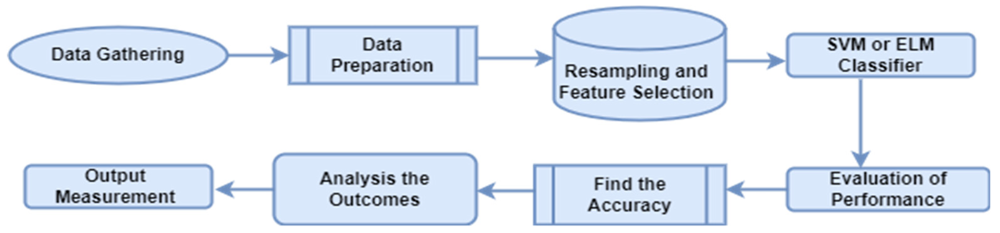
3. Proposed Methodology

The ELM and SVM classifiers were used to predict software reliability defects.

• Data Gathering.
• Data Preparation.
• Resampling and Feature Selection Methodology.
• Training the SVM classifier.
• Training the ELM classifier.
• Proposed Model and Algorithms for calculating the accuracy and time.
• Results and analysis.

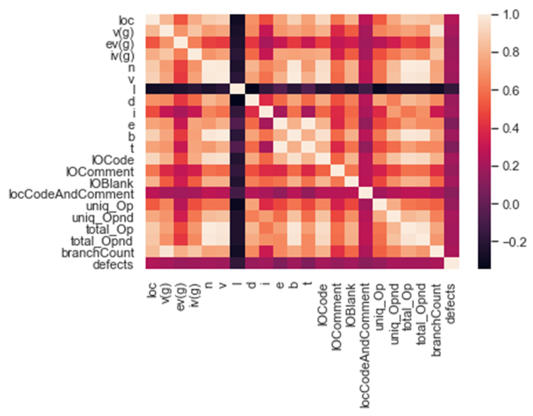
3.1. Data Gathering

The methodology of estimating, gathering, and assessing the right experiences for research utilizing spread-out approved techniques is referred to as information gathering. Because of the real factors accumulated, an expert could survey their hypothesis. No matter what the concept may be, data gathering is commonly the primary and most important stage in the research cycle. Depending on the required information, different ways of managing data gathering are used in different studies. The NASA Metrics Data Program informational index is procured through the PROMISE library. In this informational index, there are 10,885 cases with 22 properties each. A flawed dataset from NASA [61] was used to predict software problems. Source code extractors were included in Halstead’s Data Processing Program, while McCabe’s flight program provided data for an earth-orbiting satellite. The different features of the datasets are lOCode, v(g), lOComment, ev(g), locCode and Comment, iv(g), uniq_Op, n, uniq_Opnd, v, total_Op, l, total_Opnd, d, branch count, I, defects, t, e, loc, b respectively. Figure 1 depicts the proportion of the false and true values of the NASA dataset.

3.2. Data Preparation

Cleaning and altering raw information before handling and investigating are referred to as information arrangements. A critical stage before handling, as a rule, involves reformatting information, making information rectifications, and incorporating informational indexes to advance information. For data experts or business clients, information readiness can be a tedious interaction, yet it is important to put data into surroundings to change it into pieces of information and decrease bias brought about by unfortunate information quality. Following the acquisition of data, we must prepare it for the next phase. The different methods of organizing and putting together data for machine learning are known as data preparation. We then rearrange the data after merging it all. The full dataset is then analyzed to check if there is any missing information. The protocol is examined using cross-validation techniques. In Figure 2, you can see the NASA dataset correlation graph. In other words, correlation is a statistic that is used to determine the degree to which two variables are related.

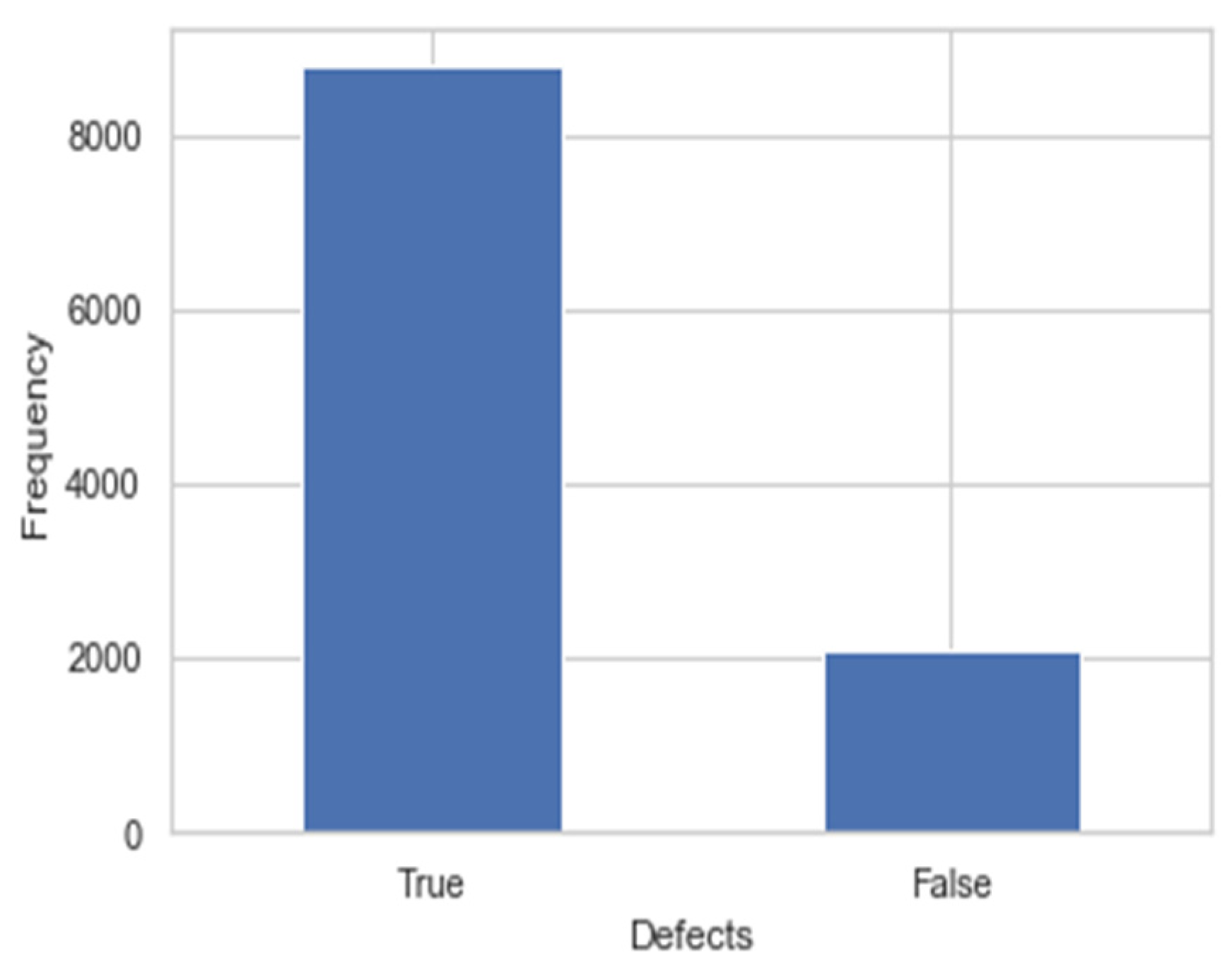
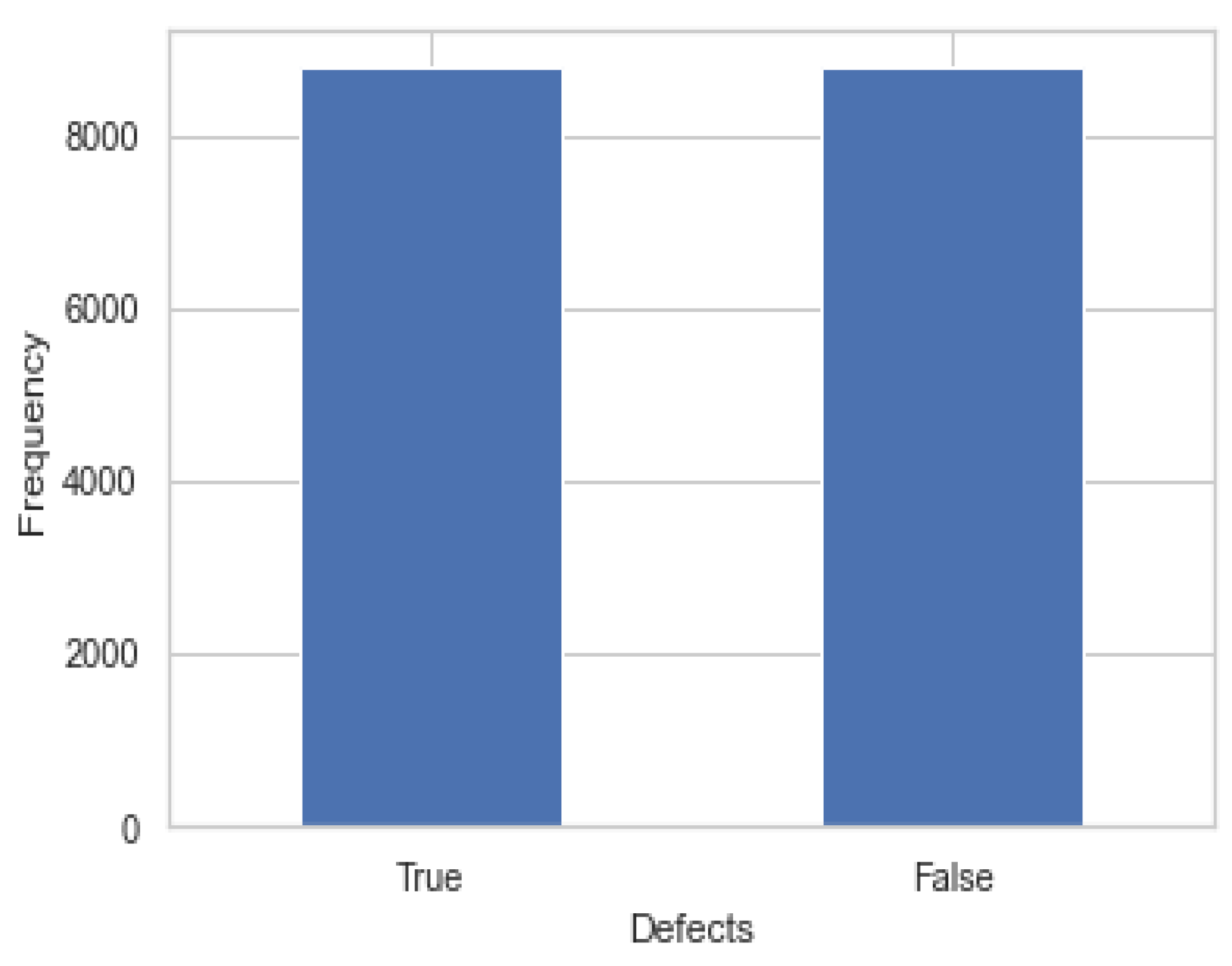
3.3. Resampling and Feature Selection Methodology

A dataset is considered imbalanced if there is a significant skew in the class distribution, such as a ratio of 1:1000 or 1:10,000 samples from the minority class to the majority class. Some machine learning algorithms may completely disregard the minority class as a result of this bias in the training dataset, which can affect various machine learning methods. This is a concern because projections are often made with the minority class in mind. Resampling the training dataset at random is one method for addressing the issue of class imbalance. Resampling can be performed in a variety of ways, including oversampling and under sampling. Choosing the most important features to input into AI algorithms is one of the primary components of feature engineering. Different feature selection methods are utilized to reduce the number of information factors by removing additional or irrelevant aspects and decreasing the scope of features to those that are generally helpful to the AI model. The following are the key advantages of pre-selecting attributes rather than relying on a machine learning model to figure out which ones are the most important. A model that is overly complicated to grasp is useless. The time it takes to train a model decreases when a more precise subset of features is used. Increasing the precision of forecasts for a given simulation. According to the dimensionally cursed phenomenon, as dimensionality and the total number of features increase, the volume of space expands so rapidly that the amount of data available diminishes. Data scientists can use feature selection to their advantage. Knowing how to select relevant qualities is critical to the algorithm’s effectiveness in machine learning. Irrelevant, redundant, and noisy features can cause a learning system to slow down, lowering performance, accuracy, and processing costs. When the typical dataset expands in size and complexity, feature selection becomes increasingly crucial. Two of the most popular feature selection techniques are Kbest and ANOVA. In this investigation, we apply the Kbest feature selection. It was found after assessing the work on highlight choice, getting an optimal subset of pertinent and non-repetitive attributes is a troublesome issue. Most existing techniques in the literature depend on univariate positioning, which disregards associations between factors previously remembered for the chosen subsets and the excess ones, neglects the dependability of the determination calculation, and strategies that produce great accuracy. Figure 3 depicts the proportion of the false and true values of the NASA dataset after using the resampling method.

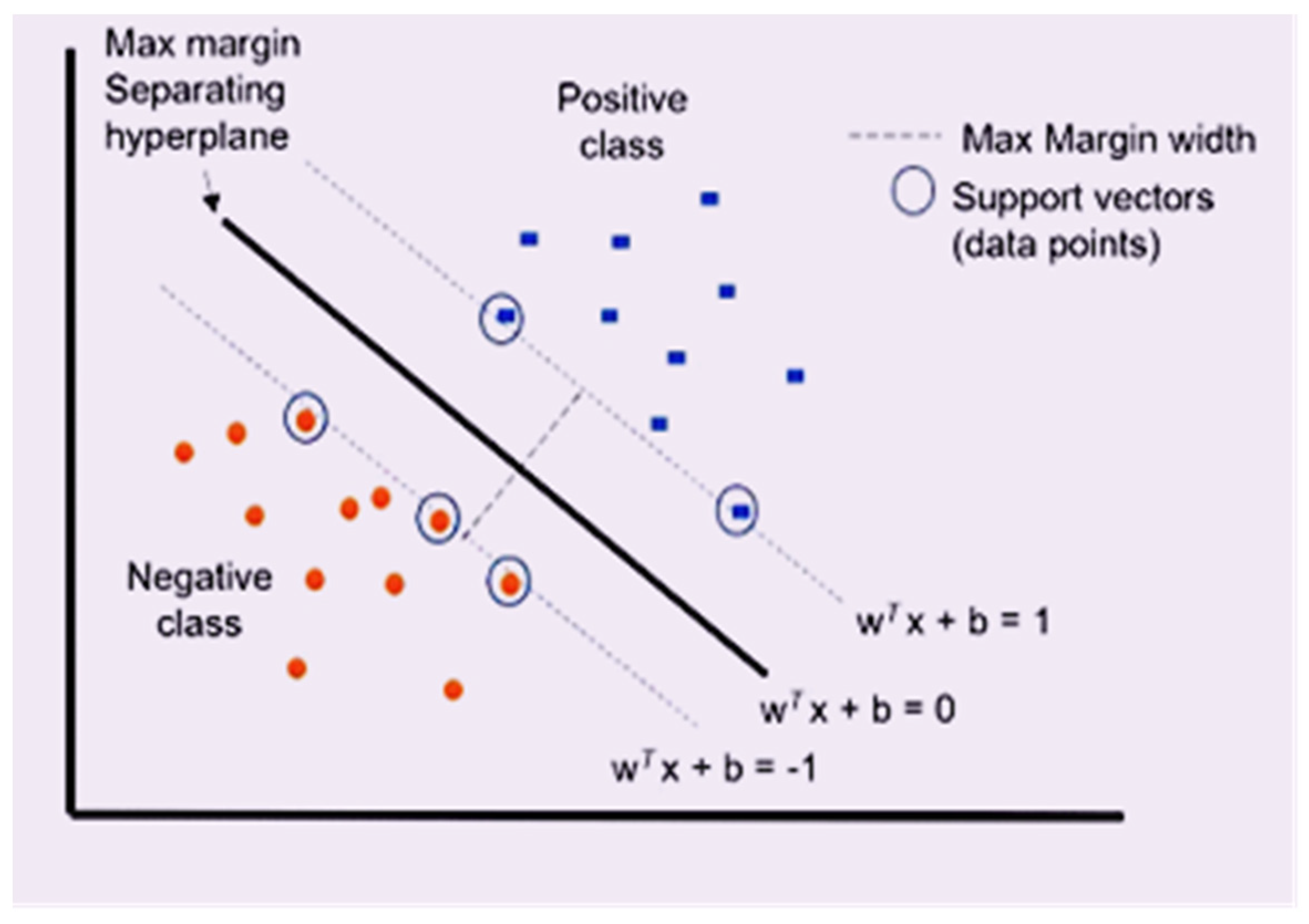
3.4. Training the SVM Classifier

SVM [62] contrasts with other classification algorithms in that it selects a choice limit that enhances the distance between every one of the classes closest to the data points. The maximum margin hyperplane is the decision border laid out by SVMs. A direct SVM classifier makes a straight line between two classes. That is, each of the useful pieces of information on one side will be assigned to a particular classification, while the data points on the opposite or another side will be assigned to another one. This suggests that the number of lines accessible is unlimited. The linear SVM calculation is better than other algorithms, for example, k-nearest neighbors, since it chooses the optimum line for characterizing the different data points. It chooses the line that partitions the information and is the farthest from the nearest data points. A 2-D illustration explains the language behind the AI. Generally, you have a matrix of pieces of data points. You are endeavoring to sort these data points into the appropriate categories, but you do not want any data to be misplaced. That is, you are looking for a line that connects the two closest points and keeps the remaining data points apart. Handwriting recognition, face detection, intrusion detection, gene classification, email classification, and web page classification are all examples of applications that use SVMs. SVMs are utilized in AI for a variety of reasons. It can deal with both linear and non-linear information for classification and regression. Another explanation for why we use SVMs is that they might find unpredictable relationships in your information without expecting you to input various changes. While working with the smallest datasets with tens to a huge number of elements, this is a brilliant option. As a result, to deal with complex and small datasets, they frequently track down additional exact responses when compared to other methods. Let us look at some of the most common kernels for which an SVM classifier can be used. The kernel function is used for converting a lower dimension to a higher dimension.

• Linear   f(X) = w^T × X + b

w, X, and b indicate the weight vector to minimize, data to classify, and the linear coefficient estimated from the training data in this equation, respectively.

• Polynomial   f(X1, X2) = (a + X1T × X2) b

f(X1, X2) represents the polynomial decision boundary that will split our data.

• Gaussian RBF   f(X1, X2) = exp (−γ || X1 − X2 ||) 2

In this equation, the gamma parameter describes the impact of a particular training point on the data points around it. Between your features, ||X1 − X2|| indicates the dot product.

To get the best accuracy, the data are separated into 70/30 training/test proportions. To increase the performance of a system, 15 percent of the training data utilized is used for validation. The values of the weight of each input parameter were merged with bios in iterative random choice tests to reduce inaccuracy. Using the support vector machine training strategy is used to depress the time data, which is part of the core internal time-related part of programming succession. After each new emphasis of a new software failure sequence, the SVM preparing method is continually and iteratively different from discovering the recent property hidden behind the software failure behavior [34]. Figure 4 shows how kernels are used in the SVM classifier.

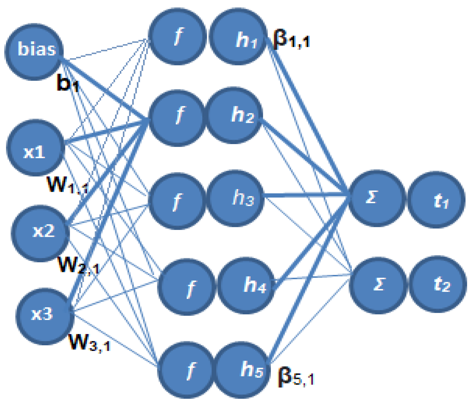
3.5. Training the ELM Classifier

Using an ELM (as illustrated in Figure 5 below) to train SLFN (Single Hidden Layer Feed-Forward Neural Networks) networks is rapid. The model’s hidden layer, which is made up of one layer of non-linear neurons, is referred to as single. The input layer supplies data features but does not compute, whereas the output layer is bias-free and linear.

Weights and biases are arbitrarily allocated to input layers and stay constant in the ELM approach. This is because the weights of input are constant and fixed, and the solution is simple and does not require iteration. For a particular linear output layer, such an answer is both straightforward and quick to compute. Because they provide nearly symmetrical hidden layer highlights, arbitrary information or input layer loads increase the speculative qualities of a linear output layer solution even further. A linear system’s solution is always made up of a collection of inputs. When the solution’s weight range is restricted, symmetrical information sources result in a bigger arrangement of space volume. As a result, the arbitrary hidden layer creates feebly connected hidden layer features, producing a low norm and high generalization accuracy solution. Because of its high prevalence in training performance, speed, and generalization, the ELM has been utilized in a wide range of applications, including medical, chemical, transportation, economics, robotics, and so on. Activation methods for the elm algorithm include ReLU, sigmoid, sin, tanh, and Leaky ReLU. In our experiment, we use the ReLU function.

We will compare and analyze the sigmoid (logistic) activation function with other activation functions such as tanh, ReLU, Leaky ReLU, and Softmax activation functions in this post. All of these are activation functions that are commonly employed in deep learning and neural network algorithms. To tackle a categorization problem, there are several algorithms on the market. One of these, the neural network, is well-known for accurately predicting data. It does, however, take a long time to compute. It is based on how neural systems process biological information. It is made up of associated layers of nodes, or we can say neurons. Information is sent to the hidden levels from the input layer. Initially, we multiply all inputs by the weights and then add a bias and apply an activation function to the result, and finally transfer the output to the next layer. This process continues until the final layer is reached. Non-linear activation functions are commonly used in neural networks, and they can aid the network in learning complex data, computing and learning nearly any function that represents a question and making correct predictions. Since they have a derivative function associated with the sources of info, they permit back-propagation.

The sigmoid activation work is a straightforward function that takes a particular real value as info and returns a probabilistic value that is somewhere in the range of 0 and 1 all of the time. It has the state “S”. It has a set result range and is non-linear and differentiable. The principal benefit is that it is clear and reasonable for use with a classifier. However, because the function’s fact that the capacity’s result is not zero focused, it causes an issue known as “vanishing gradients” It causes the angle updates to diverge too much. It is tougher to optimize when you have a 0 output and a 1. In a hidden layer of a neural network, this takes a long time to compute. Tanh can assist with sigmoid function non-zero-centered problems. Tanh reduces a real-valued number in a range between −1 and 1. In addition, it is non-linear. The derivative function is nearly identical to the derivative function of a sigmoid. It overcomes the sigmoid’s flaw; however, it cannot eliminate the vanishing gradient issue. This diagram shows how the tanh activation function compares to the sigmoid. This is the most commonly utilized activation function in NN’s hidden layer. It is not linear, despite its name and look, and offers similar advantages as sigmoid, however, with superior performance. It avoids and corrects the disappearing gradient problem issue, as well as being less computationally costly than tanh and sigmoid, these are the key advantages. In any case, it is not without defects. During preparation, certain slopes can become delicate and pass on. Subsequently, neurons start to die. As such, the weight will not be adjusted during the drop because the gradient for activations in the ReLU regionX0 () will be 0. That is, neurons in this state will no longer respond to changes in error and input. Therefore, choosing an activation function ought to be finished with an alert, and the function should be tailored to the needs of the organization. It eliminates the problem of dying ReLUs. Because this ReLU variation includes a certain small incline in the negative region, it permits back-propagation even with negative input values. For negative information esteems, the Leaky ReLU does not make solid expectations. If the learning rate is set excessively high during the front propagation, the neuron will overshoot and pass on. The concept of a Leaky ReLU can be further developed. We can multiply X x with a hyper-parameter instead of a constant term, which appears to function better with the Leaky ReLU. In general, we utilize the function in the very last layer of a neural network to calculate the distribution of probabilities to an event over a set of “n” occurrences. The ability to handle various classes is the function’s key benefit.

3.6. Proposed Model and Algorithm for Calculating the Accuracy and Time

We construct a proposed Algorithm 1 for calculating the accuracy in this area of our paper, and we also find time to execute the approach in this section. In this case, we used the SVM classifier first and, subsequently, the ELM classifier in the NASA dataset. We compare the results at last. Figure 6 illustrates a proposed prediction model after using feature selection with SVM and ELM classifiers. The different methods are used in this model, i.e., data gathering, data preparation, and feature selection using Kbest, implementing SVM or ELM classifier, evaluation of performance, finding the accuracy, and analysis of outcomes at the last output measurement.

Algorithm 1 Calculating the accuracy and time

Input:  NASA Dataset Output:  To improve precision and reliability Step-1  Begin Step-2  Import NASA’s data. Step-3  NASA dataset pre-processing features Step-4  Implement the Resampling MethodStep-4 Implement the Method of Feature Selection Step-5  Then, for hyper-parameter analysis, we used SVM or ELM classifiers on our          Dataset with various functions. Step-6  Our model then concentrates on Hyper-plane. Step-7  Calculate the accuracy and time. Step-8  End

The initial stage in our strategy is gathering data for the ML model’s training, which is the fundamental machine learning step. Only the data used to train the models can guarantee the accuracy of the predictions. There are a variety of issues that can arise during the data collection process, such as the fact that the data collected may not be relevant to the problem statement (inaccurate data), empty values in columns, missing images for some classes of predictions (missing data), data imbalance, and private data. The pre-processing or preparation of our data comes next. There are several methods for performing this, including data imputations using the standard deviation, mean, median, and k-nearest neighbors (k-NN) of the data in the given field; bias or imbalance in the dataset can be corrected by repetition, bootstrapping, or synthetic minority over-sampling technique (Oversampling) or data integration. Additionally, in this stage, we partitioned our dataset into training and testing portions. Following the removal of unnecessary features from our datasets using the feature selection approach, the cleaned data are fed into the classifier to build our model. Our model calculates various characteristics, including accuracy, specificity, recall, and precision, after calculating the confusion matrix, which is comprised of the true positive, true negative, false positive, and false negative outcomes. We use SVM and ELM classifiers in our experiment. At the time of our experiment, we carefully observe each parameter after constructing a distinct classifier.

3.7. Testing and Calculation of Accuracy

A test’s accuracy is still up in the air due to its capacity to suitably recognize healthy and sick cases. To calculate the part of true negative (−ve) and true positive (+ve) cases in every analyzed case, we need to calculate the test data accuracy. Accuracy calculation depends upon the four parameters of the confusion matrix i.e FP, TP, TN, and FN. The different number of instances correctly identified are false positives (FP), and true positives (TP) is the number of misidentified cases. The number of attributes correctly classified is called a true negative (TN). The number of attributes wrongly classified is called a false negative (FN).

The ELM classifier’s accuracy and time computation improved after this test on the NASA dataset. We will provide an accuracy table once we have finished all of the procedures. The accuracy calculations for both approaches are compared in

Table 1. Accuracy and Time Calculation Table.

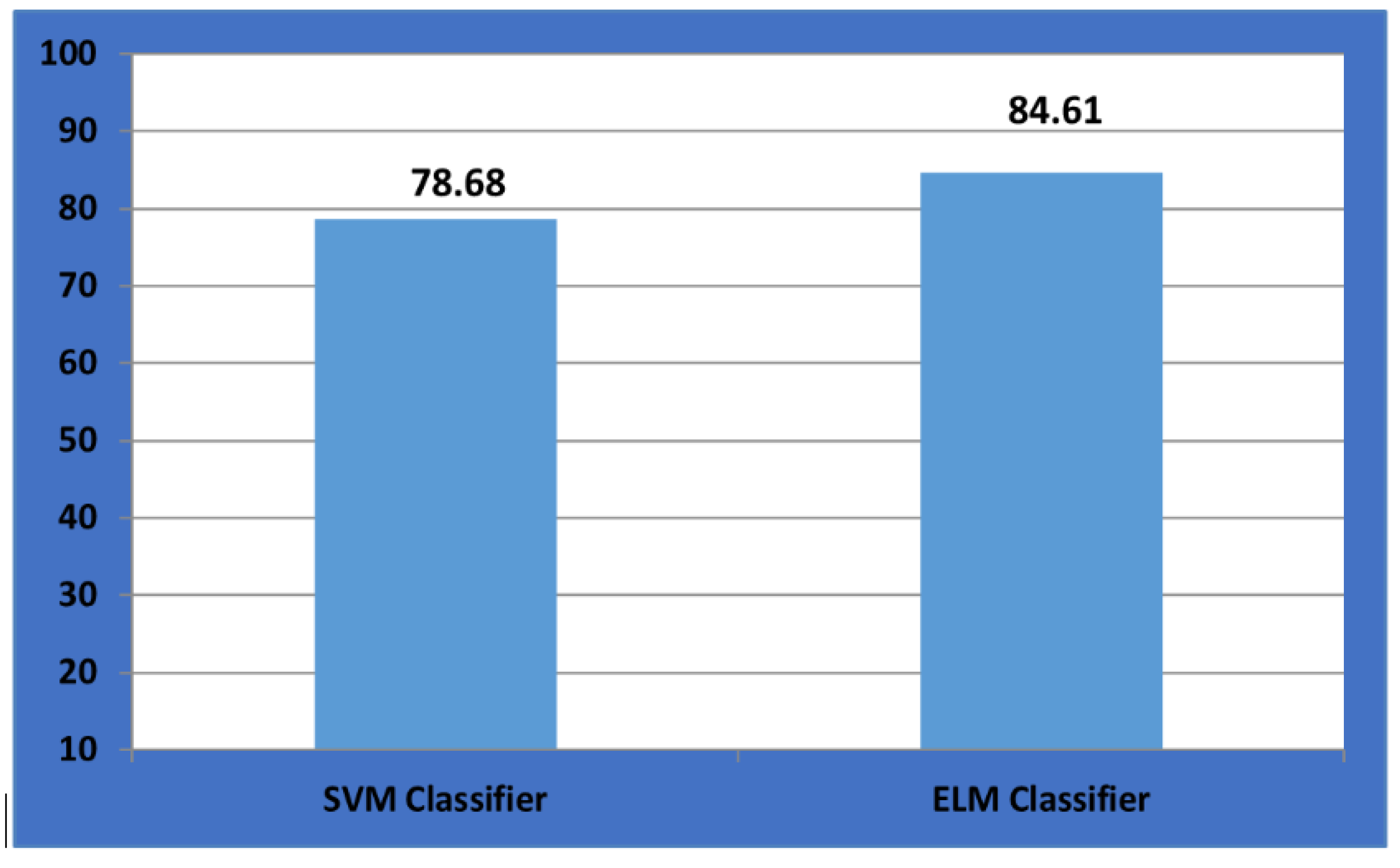
Input	Accuracy Calculated Using SVM Classifier	Accuracy Calculated Using ELM Classifier	Time Required For Execution of SVM Classifier	Time Required for Execution of ELM Classifier
NASA dataset	0.7868965517241	0.84617241379310	2.8329972743988037 s	0.6670020008087158 s

. Further,

Table 2. F1-measure, Precision, Recall, and Specificity Calculation Table (Using SVM).

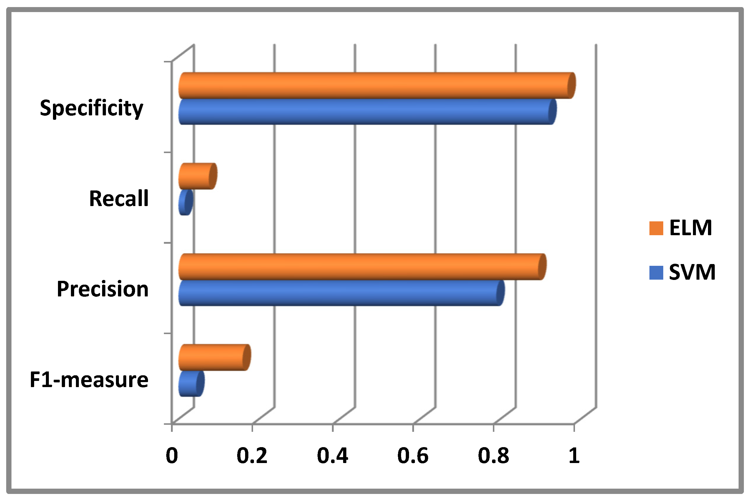
Input	F1-Measure Calculated Using SVM Classifier	Precision Calculated Using SVM Classifier	Recall Calculated Using SVM Classifier	Specificity Calculated Using SVM Classifier
NASA dataset	0.043638	0.79	0.015163	0.919331

and

Table 3. F1-measure, Precision, Recall, and Specificity Calculation Table (Using ELM).

Input	F1-Measure Calculated Using ELM Classifier	Precision Calculated Using ELM Classifier	Recall Calculated Using ELM Classifier	Specificity Calculated Using ELM Classifier
NASA dataset	0.158019	0.894939	0.075128	0.966846

represent the value of other parameters, such as specificity, recall, precision, and F1-measure.

4. Results and Analysis

We used two methods in our experiment: SVM classifier and ELM classifier. That is, we use SVM to classify our NASA dataset before getting 78.68 percent accuracy. The accuracy of the next technique is raised to 84.61 percent by applying ELM classification to the NASA dataset. We may also compare the execution time; for example, SVM classification takes more than 2 s while Elm classification takes less than 1 s. Table 1 compares the accuracy and execution time of the two approaches. Figure 7 illustrates a portion of our implementation code for calculating the accuracy and time for SVM and ELM. We employed numerous types of parameters in our experiment, such as ANOVA and Kbest, in feature selection strategies. Different parameters, such as ReLU, sigmoid, sin, and tanh, are also tested in the ELM approach. We are taking those parameters and creating a model based on them. Figure 7 illustrates the accuracy comparison graph. The accuracy provided by the SVM classifier will always be greater than the value provided by the ELM classifier in each iteration. To make it easier to compare with the SVM model in our experiment, we calculated the average from all of the iteration values of ELM.

Figure 8 illustrates that Elm not only gets a higher accuracy as compared with SVM but also it will get the best result for other parameters such as specificity, recall, precision, and F1-measure.

5. Conclusions and Future Work

This study compares and analyzes two classification methods that are similar as far as accuracy and duration go. The ELM and SVC classifiers are implemented in this study using the NASA dataset. The NASA benchmark dataset can be found in the Promise data repository, which is available to the public for research to determine which methodology is superior of the two algorithms. The ELM classifier model is the most accurate. The ELM technique also takes less time than the SVM classifier. To improve the accuracy and save time spent on feature processing, we can utilize feature selection procedures in this classifier. In our work, we investigate the precision and computational efficiency of SVM- and ELM-based software reliability prediction models. Then, following comparison, we obtained experimental findings showing that the ELM-based reliability prediction model may reach higher prediction accuracy when combined with other factors, such as specificity, recall, precision, and F1-measure. In this paper, a paradigm for using feature selection with ELM and SVM is also put forward.

A systematic literature review on software defect prediction using machine learning is presented in this work. A large number of papers were obtained from electronic databases, and certain publications were chosen based on the study selection criteria. Platforms, machine learning types, datasets, evaluation metrics, and machine learning algorithms, validation methodologies, best machine learning, software metrics, and deep learning algorithms, problems, and gaps are all identified, with the associated results presented. Researchers overwhelmingly favored the software platform. Furthermore, software fault prediction studies have restricted several types of repositories and datasets. In software defect prediction, most of the researchers utilized object-oriented metrics. Supervised learning is utilized in the majority of the investigations as compared to unsupervised and semi-supervised learning algorithms. This indicates that there is still a need for more research into software fault prediction using unsupervised and semi-supervised learning. We intend to use these methods to create unique software and reliability models.

References

- Lecun, Y.; Bottou, L.; Bengio, Y.; Haffner, P. Gradient-based learning applied to document recognition. Proc. IEEE 1998, 86, 2278–2324. [Google Scholar] [CrossRef]
- Lawrence, S.; Giles, C.L.; Ah Chung, T.; Back, A.D. Face recognition: A convolutional neural-network approach. IEEE Trans. Neural Netw. 1997, 8, 98–113. [Google Scholar] [CrossRef] [PubMed]
- Hinton, G.E.; Salakhutdinov, R.R. Reducing the dimensionality of data with neural networks. Science 2006, 313, 504–507. [Google Scholar] [CrossRef] [PubMed]
- Hinton, G.; Osindero, S.; The, Y. A fast learning algorithm for deep belief nets. Neural Comput. 2006, 18, 1527–1554. [Google Scholar] [CrossRef]
- Salakhutdinov, R.; Hinton, G. Deep Boltzmann machines. In Proceedings of the International Conference Artificial Intelligence and Statistics, Chia Laguna Resort, Sardinia, Italy, 13–15 May 2009; pp. 448–455. [Google Scholar]
- Huang, G.B.; Lee, H.; Learned-Miller, E. Learning hierarchical representations for face verification with convolutional deep belief networks. In Proceedings of the IEEE International Computer Vision and Pattern Recognition, Providence, RI, USA, 16–21 June 2012; pp. 2518–2525. [Google Scholar]
- Sun, Y.; Wang, X.; Tang, X. Hybrid deep learning for face verification. In Proceedings of the IEEE International Conference Computer Vision, University of Science and Technology of China 2013, Sydney, Australia, 1–8 December 2013; p. 262 L. [Google Scholar]
- Taigman, Y.; Yang, M.; Ranzato, M.A.; Wolf, L. DeepFace: Closing the gap to human-level performance in face verification. In Proceedings of the IEEE International Computer Vision and Pattern Recognition, Menlo Park, CA, USA, 23–28 June 2014. [Google Scholar]
- Zhou, E.; Cao, Z.; Yin, Q. Naïve-deep face recognition: Touching the limit of LFW benchmark or not? arXiv 2015, arXiv:1501.04690. [Google Scholar]
- Cortes, C.; Vapnik, V. Support-vector networks. Mach. Learn. 1995, 20, 273–297. [Google Scholar] [CrossRef]
- Vapnik, V. The Nature of Statistical Learning Theory; Springer: New York, NY, USA, 1995. [Google Scholar]
- Huang, G.; Zhu, Q.; Siew, C. Extremelearningmachine: Theory and applications. Neurocomputing 2006, 70, 489–501. [Google Scholar] [CrossRef]
- Huang, G.; Chen, L.; Siew, C. Universal approximation using incremental constructive feedforward networks with random hidden nodes. IEEE Trans. Neural Netw. 2006, 17, 879–892. [Google Scholar]
- Haykin, S.O. Neural Networks: A Comprehensive Foundation, 2nd ed.; Prentice-Hall: Hoboken, NJ, USA, 1999. [Google Scholar]
- Funahashi, K.; Funahashi, K.I. On the approximate realization of continuous mappings by neural networks. Neural Netw. 1989, 2, 183–192. [Google Scholar] [CrossRef]
- Shanthini, A. Effect of ensemble methods for software fault prediction at various metrics level. In International Journal of Applied Information Systems (IJAIS); Foundation of Computer Science FCS: New York, NY, USA, 2013. [Google Scholar]
- Xia, X.; Lo, D.; McIntosh, S.; Shihab, E.; Hassan, A.E. Cross-Project Build Co-Change Pre-Diction. In Proceedings of the IEEE 22nd International Conference on Software Analysis, Evolution and Reengineering (SANER), Gold Coast, Australia, 9–12 December 2015; pp. 311–320. [Google Scholar]
- Yang, F.-J. An Implementation of Naive Bayes Classifier. In Proceedings of the 2018 International Conference on Computational Science and Computational Intelligence (CSCI), Las Vegas, NV, USA, 12–14 December 2018; pp. 301–306. [Google Scholar] [CrossRef]
- Elish, K.O.; Elish, M.O. Predicting defect-prone software modules using support vector machines. J. Syst. Softw. 2008, 81, 649–660. [Google Scholar] [CrossRef]
- Yan, Z.; Chen, X.; Guo, P. Software defect prediction using fuzzy support vector regression. Adv. Neural Netw. 2010, 6064, 17–24. [Google Scholar]
- Jing, X.; W, F.; Dong, X.; Qi, F.; Xu, B. Heterogeneous cross-company defect prediction by unified metric representation and CCA-based transfer learning. In Proceedings of the 10th Joint Meeting on Foundations of Software Engineering (FSE), ACM, Bergamo, Italy, 30 August–4 September 2015; pp. 496–507. [Google Scholar]
- Goel, A.L. A Guidebook for Software Reliability Assessment; Rep. RADCTR-83-176; Syracuse University: New York, NY, USA, 1983. [Google Scholar]
- Knab, P.; Pinzger, M.; Bernstein, A. Predicting defect densities in source code files with decision tree learners. In Proceedings of the 3rd International Workshop on Mining Software Repositories (MSR), ACM, Shanghai, China, 22–23 May 2006; pp. 119–125. [Google Scholar]
- Thwin, M.M.T.; Quah, T.-S. Application of neural networks for software quality prediction using object-oriented metrics. J. Syst. Softw. 2005, 76, 147–156. [Google Scholar] [CrossRef]
- Khoshgoftaar, T.M.; Allen, E.B.; Hudepohl, J.P.; Aud, S.J. Application of neural networks to software quality modeling of a very large telecommunications system. IEEE Trans. Neural Netw. 1997, 8, 902–909. [Google Scholar] [CrossRef] [PubMed]
- Neumann, D.E. An enhanced neural network technique for software risk analysis. IEEE Trans. Soft. Eng. 2002, 28, 904–912. [Google Scholar] [CrossRef]
- Panichella, A.; Oliveto, R.; de Lucia, A. Cross-project defect prediction models: L’union fait la force. In Proceedings of the IEEE 21st Software Evolution Week-IEEE Conference on Software Maintenance, Reengineering and Reverse Engineering (CSM- R-WCRE), Antwerp, Belgium, 3–6 February 2014; pp. 164–173. [Google Scholar]
- Boetticher, G.; Menzies, T.; Ostrand, T. PROMISE Repository of Empirical Software Engineering Data; West Virginia University, Department of Computer Science: Morgantown, WV, USA, 2007. [Google Scholar]
- Leo, M.; Sharma, S.; Maddulety, K. Machine learning in banking risk management: A literature review. Risks 2019, 7, 29. [Google Scholar] [CrossRef]
- Boughaci, D.; Alkhawaldeh, A.A. Appropriate machine learning techniques for credit scoring and bankruptcy prediction in banking and finance: A comparative study. Risk Decis Anal. 2020, 8, 15–24. [Google Scholar] [CrossRef]
- Kou, G.; Chao, X.; Peng, Y.; Alsaadi, F.E.; Herrera-Viedma, E. Machine learning methods for systemic risk analysis in financial sectors. Technol. Econ. Dev. Econ. 2019, 25, 716–742. [Google Scholar] [CrossRef]
- Beam, A.L.; Kohane, I.S. Big data and machine learning in health care. JAMA 2018, 319, 1317–1318. [Google Scholar] [CrossRef]
- Char, D.S.; Shah, N.H.; Magnus, D. Implementing machine learning in health care Addressing ethical challenges. N. Engl. J. Med. 2018, 378, 981. [Google Scholar] [CrossRef]
- Panch, T.; Szolovits, P.; Atun, R. Artificial intelligence, machine learning, and health systems. J. Glob. Health 2018, 8, 020303. [Google Scholar] [CrossRef] [PubMed]
- Stone, P.; Veloso, M. Multiagent systems: A survey from a machine learning perspective. Auton Robots 2000, 8, 345–383. [Google Scholar] [CrossRef]
- Mosavi, A.; Varkonyi, A. Learning in robotics. Int. J. Comput. Appl. 2017, 157, 8–11. [Google Scholar] [CrossRef]
- Polydoros, A.S.; Nalpantidis, L. Survey of model-based reinforcement learning: Applications on robotics. J. Intell. Robot. Syst. 2017, 86, 153–173. [Google Scholar] [CrossRef]
- Bhavsar, P.; Safro, I.; Bouaynaya, N.; Polikar, R.; Dera, D. Machine learning in transportation data analytics. In Data Analytics for Intelligent Transportation Systems; Elsevier: Amsterdam, The Netherlands, 2017; pp. 283–307. [Google Scholar]
- Zantalis, F.; Koulouras, G.; Karabetsos, S.; Kandris, D. A review of machine learning and IoT in smart transportation. Future Internet 2019, 11, 94. [Google Scholar] [CrossRef]
- Ermagun, A.; Levinson, D. Spatiotemporal traffic forecasting: Review and proposed directions. Transp. Rev. 2018, 38, 786–814. [Google Scholar] [CrossRef]
- Ballestar, M.T.; Grau-Carles, P.; Sainz, J. Predicting customer quality in e-commerce social networks: A machine learning approach. Rev. Manag. Sci. 2019, 13, 589–603. [Google Scholar] [CrossRef]
- Rath, M. Machine Learning and Its Use in E-Commerce and E-Business. In Handbook of Research on Applications and Implementations of Machine Learning Techniques; IGI Global; Birla Global University: Odisha, India, 2020; pp. 111–127. [Google Scholar]
- Kohavi, R.; John, G.H. Wrapper for Feature Subset Selection; Artificial Intelligence; Elsevier: Amsterdam, The Netherlands, 1997; pp. 273–324. [Google Scholar]
- Shivaji, S.; Whitehead, E.J.; Akella, R.; Kim, S. Reducing features to improve code change-based bug prediction. IEEE Trans. Softw. Eng. 2013, 39, 552–569. [Google Scholar] [CrossRef]
- Blum, A.L.; Rivest, R.L. Training a 3-node neural networks is NP-complete. Neural Netw. 1992, 5, 117–127. [Google Scholar] [CrossRef]
- Liu, H.; Motoda, H. Feature Selection for Knowledge Discovery and Data Mining; Kluwer Academic Publishers: Boston, MA, USA, 1998. [Google Scholar]
- Song, Q.; Jia, Z.; Shepperd, M.; Ying, S.; Liu, J. A general software defect-proneness prediction framework. IEEE Trans. Softw. Eng. 2011, 37, 356–370. [Google Scholar] [CrossRef]
- Shivaji, S.; Whitehead, J.E.J.; Akella, R.; Kim, S. Reducing features to improve bug prediction. In Proceedings of the 24th International Conference on Automated Software Engineering (ASE), Auckland, New Zealand, 16–20 November 2009; IEEE Computer Society: Washington, DC, USA, 2009; pp. 600–604. [Google Scholar]
- Elmurngi, E.; Gherbi, A. An empirical study on detecting fake reviews using machine learning techniques. In Proceedings of the IEEE 2017 Seventh International Conference on Innovative Computing Technology (INTECH), Luton, UK, 16–18 August 2017; pp. 107–114. [Google Scholar]
- Wold, S.; Esbensen, K.; Geladi, P. Principal component analysis, Chemom. Intell. Lab. Syst. 1987, 2, 37–52. [Google Scholar] [CrossRef]
- Gao, K.; Khoshgoftaar, T.M.; Wang, H.; Seiya, N. Choosing software metrics for defect prediction: An investigation on feature selection techniques. Softw. Pract. Exp. 2011, 41, 579–606. [Google Scholar] [CrossRef]
- Chen, X.; Shen, Y.; Cui, Z.; Ju, X. Applying feature selection to software defect prediction using multi-objective optimization. In Proceedings of the IEEE 41st Annual Computer Software and Applications Conference (COMPSAC), Turin, Italy, 4–8 July 2017; pp. 54–59. [Google Scholar]
- Catal, C.; Diri, B. Investigating the effect of dataset size, metrics sets, and feature selection techniques on software fault prediction problem. Inf. Sci. 2009, 179, 1040–1058. [Google Scholar] [CrossRef]
- Vandecruys, O.; Martens, D.; Baesens, B.; Mues, C.; Backer, M.D.; Haesen, R. Mining software repositories for comprehensible software fault prediction models. J. Syst. Softw. 2008, 81, 823–839. [Google Scholar] [CrossRef]
- Czibula, G.; Marian, Z.; Czibula, I.G. Software defect prediction using relational association rule mining. Inf. Sci. 2014, 260–278. [Google Scholar] [CrossRef]
- Mahaweerawat, A.; Sophatsathit, P.; Lursinsap, C.; Musilek, P. MASP-An enhanced model of fault type identification in object-oriented software engineering. J. Adv. Comput. Intell. Intell. Inform. 2006, 10, 312–322. [Google Scholar] [CrossRef]
- Gondra, I. Applying machine learning to software fault-proneness prediction. J. Syst. Softw. 2008, 81, 186–195. [Google Scholar] [CrossRef]
- Menzies, T.; Greenwald, J.; Frank, A. Data mining static code attributes to learn defect predictors. IEEE Trans. Softw. Eng. 2007, 33, 2–13. [Google Scholar] [CrossRef]
- Van Heeswijk, M.; Miche, Y.; Lindh-Knuutila, T.; Hilbers, P.A.; Honkela, T.; Oja, E.; Lendasse, A. Adaptive ensemble models of extreme learning machines for time series prediction. Lect. Notes Comput. Sci. 2009, 5769, 305–314. [Google Scholar]
- Rong, H.-J.; Ong, Y.-S.; Tan, A.-H.; Zhu, Z. A fast pruned extreme earning machine for classification problem. Neurocomputing 2008, 72, 359–366. [Google Scholar] [CrossRef]
- Dash, M.; Liu, H. Feature Selection for Classification; Intelligent Data Analysis; Elsevier: Amsterdam, The Netherlands, 1997; pp. 131–156. [Google Scholar]
- Rath, S.K.; Sahu, M.; Das, S.P.; Mohapatra, S.K. Hybrid Software Reliability Prediction Model Using Feature Selection and Support Vector Classifier. In Proceedings of the 2022 International Conference on Emerging Smart Computing and Informatics (ESCI), Pune, India, 9–11 March 2022; pp. 1–4. [Google Scholar] [CrossRef]