Addressing a New Class of Multi-Objective Passive Device Optimization for Radiofrequency Circuit Design

Abstract

The design of radiofrequency circuits and systems lends itself to multi-objective optimization and the bottom-up composition of Pareto-optimal fronts. Conventional multi-objective optimization algorithms can effectively attain these fronts, which maximize or minimize a set of competing objective functions of interest. However, some of these real-life optimization problems reveal a non-conventional feature: there is one objective function that calls neither for minimization nor maximization. Instead, using the Pareto front demands this objective function to be swept across so that all its feasible values are available. Such a non-conventional feature, as shown here, emerges in the case of inductor optimization. The problem thus turns into a non-conventional one: determining how to find uniformly distributed feasible values of this function over the broadest possible range (typically unknown) while minimizing or maximizing the remaining competing objective functions. An NSGA-II-inspired algorithm is proposed that, based on the dynamic allocation of objective function slots and a modified dominance definition, can successfully return sets of solutions for inductor optimization problems with one sweeping objective. Furthermore, a mathematical benchmark function modeling this kind of problem is presented, which is also used to exhaustively test the proposed algorithm and obtain insight into its parameter settings.

1. Introduction

Optimization has been widely applied to many electronic design problems over the past 30 years [1,2,3,4]. Circuit design problems are well suited to mathematical optimization because most performances of interest can be posed as the minimization and/or maximization of a set of objectives subject to several constraints. Although most circuit design problems are essentially constrained multi-objective optimization problems, they are usually transformed into single-objective optimization problems by a weighted addition of objectives, together with a constraint-handling mechanism [5].

In the past 20 years, however, the availability of multi-objective optimization algorithms has provided new alternatives in multiple engineering applications [6], particularly in electronic design, having considerable success in the design of analog, mixed-signal and radiofrequency (AMS/RF) integrated circuits [4,5,7,8,9,10,11,12,13,14]. Not only are these algorithms more flexible for a posteriori selection of the desired trade-off among two or more circuit performances, but they also have enabled new design paradigms based on the bottom-up composition of Pareto-optimal fronts at different hierarchical levels [9,12,13]. In these approaches, complex circuits are hierarchically decomposed into smaller sub-blocks, and solutions with the best trade-offs among competing objectives of lower level blocks (i.e., an approximation to their Pareto front) are used as the decision space of higher level blocks. In this way, Pareto fronts are composed up the hierarchy. Figure 1 illustrates the bottom-up design methodology of a hierarchy with three levels. At the lowest level, the Pareto fronts of the different sub-blocks are first generated. Although illustrated in Figure 1 for two-dimensional fronts, the number of dimensions may change from one sub-block to another. Then, the solutions in these Pareto fronts become the decision space for the optimization processes at the following level (Sub-block 1 to Sub-block N in Figure 1). These optimization processes yield Pareto fronts at this level, whose solutions, in turn, constitute the decision space for the optimization process at the system level. These approaches have been applied to the synthesis of data converters or phase-locked loops [9], and, in the past few years, they have been extended down to the device level for radiofrequency (RF) circuit design [10,11,12,13,14].

However, although most performances of interest can be posed as minimization or maximization objectives (e.g., the minimization of power consumption), other performances are neither maximized nor minimized. Instead, all possible values of these performances should be attained for all the other values of the minimized/maximized performances (e.g., for all minimized values of power consumption). Furthermore, the possible value ranges of those performances are not known a priori. Consider, for instance, a transconductance amplifier and assume that the performances of interest are power, transconductance, area and output impedance. Naturally, output impedance should be maximized, and power and area should be minimized. However, what should be done with the transconductance? In fact, neither maximization nor minimization is correct here. Instead, the optimal solutions are those with minimal area and power and maximal output impedance for every possible transconductance value so that the right one is selected when a composition process, as shown in Figure 1, is applied. Conventional multi-objective optimization algorithms can be applied to solve these problems if such performance (e.g., the transconductance) trades off with other circuit performances; as such, a full range of values will result from the multi-objective optimization. However, this is not always the case, and, in particular, it is not the case for inductor design in RF circuits.

In this paper, the problem is formulated, and an algorithm is proposed to solve it. The preliminary results are reported in ref. [15]. The remainder of the paper is organized as follows: Section 2 provides the motivation for the problem with details of a practical inductor design problem. The problem is formulated, and proper definitions are introduced in Section 3. Section 4 presents the proposed algorithm. Section 5 describes the experimental results from the case study in Section 2. Section 6 proposes a mathematical benchmark function that can be used for this type of optimization problem together with experimental results from the algorithm application. Performance metrics are also used. Finally, Section 7 provides the concluding remarks.

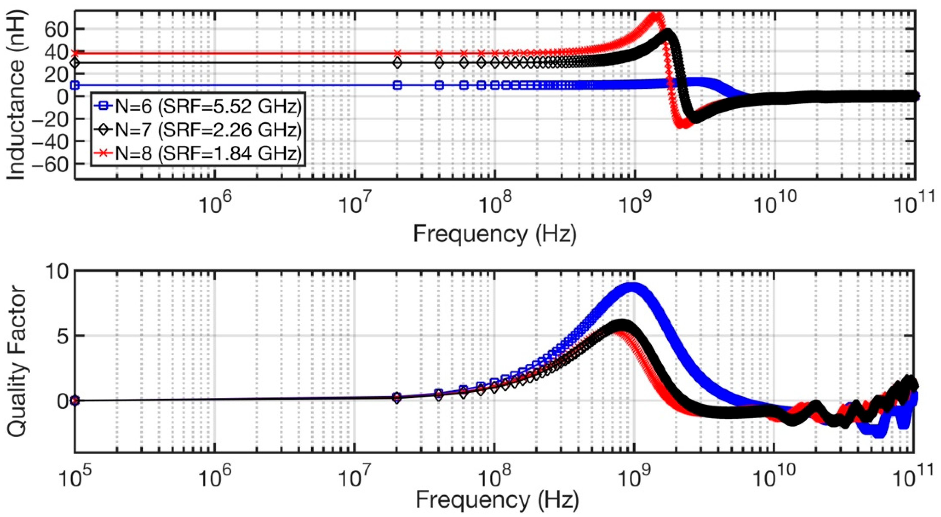
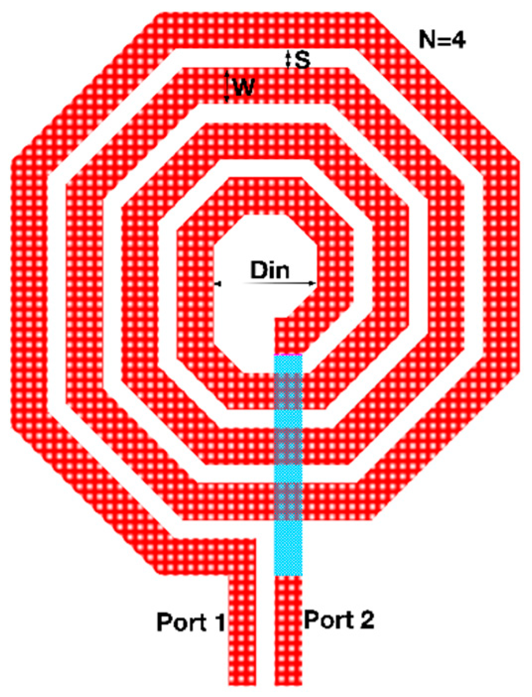
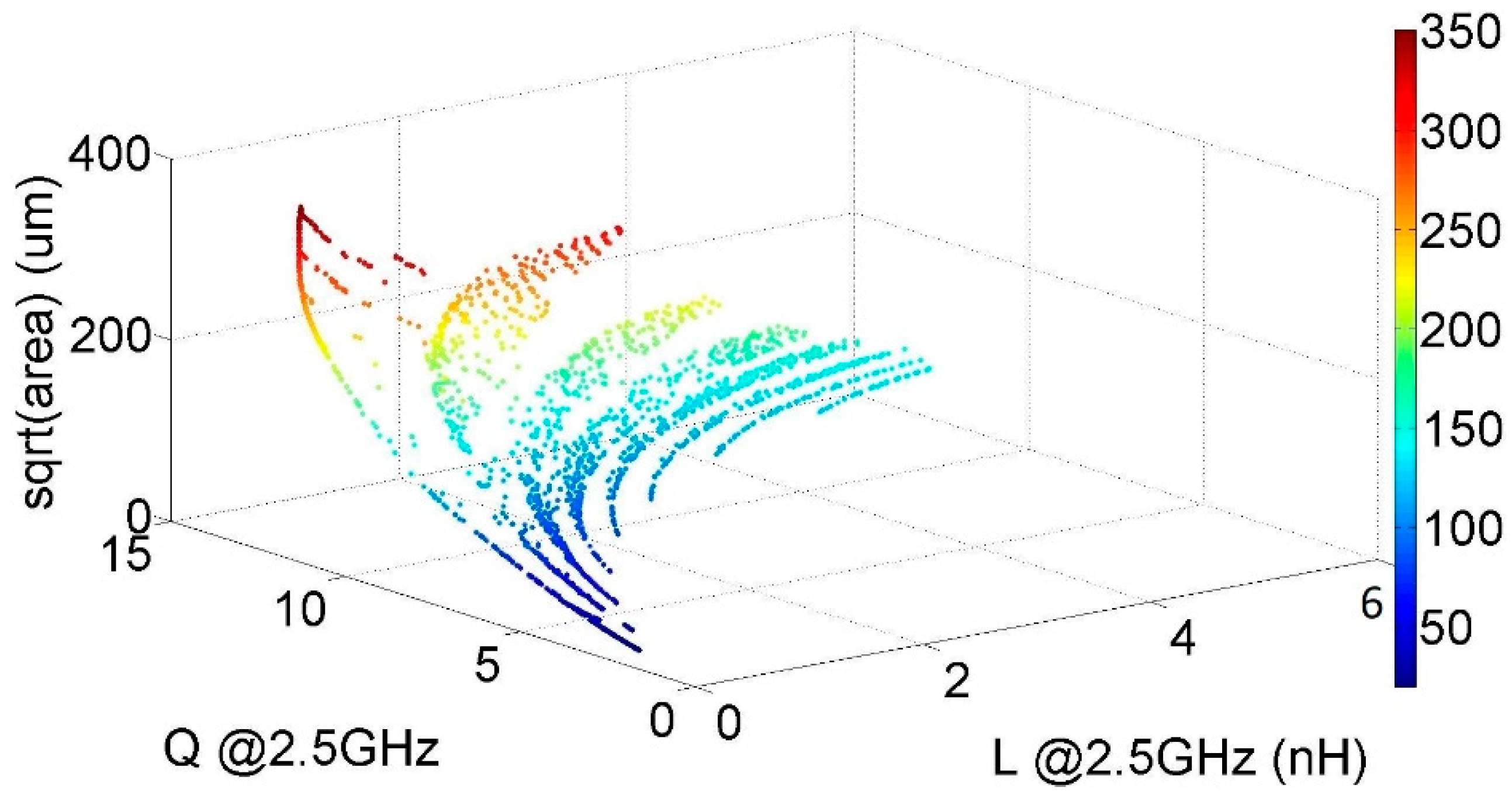
2. Inductor Design Problem

The optimization requirements for some of the electronic design problems discussed above are illustrated in this Section with one particular example: the design of RF inductors. Inductors in RF integrated circuits are typically built using two metal layers with an intermediate dielectric layer. As an illustration, Figure 2 shows the shape of an octagonal asymmetric spiral inductor. The geometry of this planar spiral inductor is usually defined by four geometric parameters: the number of turns (N), the inner diameter (D_in), the turn width (w) and the spacing between turns (s). The most relevant inductor performances are the equivalent inductance, $L_{eq}$, and the quality factor, $Q$, both a function of frequency, $\omega$. In Figure 3, three typical plots of the inductance and quality factor as a function of frequency are shown.

Let us assume that we wish to look for the best inductors that fit within a given area, denoted as area_max, for a circuit application operating at 2.5 GHz. Here, “best” means to obtain inductors with the highest quality factor for each inductance value at such frequency of operation. Note the difference between these two performances: when an inductor is selected for an RF circuit with some given specifications, a specific inductance is required, but any quality factor higher than the minimum requirement is acceptable.

In addition, two design constraints are imposed: the inductance value must be sufficiently flat from DC to slightly above the frequency of operation, and the self-resonance frequency (SRF) must be sufficiently above this frequency. Since calculating the SRF can be computationally expensive, the latter constraint is approximated by imposing that the quality factor is near its maximum at the operating frequency and has a positive slope. Given the typical inductance shape in Figure 3, the flatness of the inductance can be controlled by constraining the maximum deviation between the inductance at the frequency of operation and the inductances at a few key frequencies. Therefore, the optimization constraints are formulated as follows:

$$\left\{\begin{array}{c}area<area\_max\\ \left|\frac{L_{@2.5\mathrm{GHz}}-L_{@2.55\mathrm{GHz}}}{L_{@2.5\mathrm{GHz}}}\right|<0.01\\ \left|\frac{L_{@2.5\mathrm{GHz}}-L_{@2.45\mathrm{GHz}}}{L_{@2.5\mathrm{GHz}}}\right|<0.01\\ \left|\frac{L_{@2.5\mathrm{GHz}}-L_{@0.1\mathrm{GHz}}}{L_{@2.5\mathrm{GHz}}}\right|<0.05\\ Q_{@2.55\mathrm{GHz}}-Q_{@2.5\mathrm{GHz}}>0\end{array}\right.$$

(1)

These optimization constraints can be handled using a variety of mechanisms reported in the literature [16,17,18,19,20]. The bounds of the optimization search space are set by the design rules of the fabrication technology at the lower end and by reasonable practical values at the upper end. These are shown in

Table 1. Inductor design variables.

Parameter	Minimum	Step	Maximum
N	1	1	10
w	5 μm	0.05 μm	25 μm
Din	10 μm	0.05 μm	300 μm
s	2.5 μm	-	2.5 μm

. The spacing is fixed to 2.5 μm, as no performance improvement is expected for larger values. Although some authors have reported improvements in the quality factor by steadily increasing the width of the outer turns [21,22], the turn width has been made equal for all turns in this experiment. Due to fabrication technology constraints, the inner diameter and turn width are forced to fit on a grid of 0.05 μm.

If a conventional multi-objective optimization algorithm (e.g., based on Pareto ranking [23] or based on decomposition [24]) is applied to the maximization of inductance and the quality factor at 2.5 GHz, subject to the constraints in Equation (1), the Pareto fronts in Figure 4 are obtained for two different area constraints. The designer is typically interested in obtaining the inductor with the maximal quality factor for a given inductance. By looking at the inductance–quality factor plot in Figure 4a, it might seem that inductance values below 1.1 nH or between 1.4 nH and 2.6 nH are not achievable for inductors that fit in a 200 μm-side square. Furthermore, by looking at the front in Figure 4b, it seems that only three inductance values are achievable with this area constraint. However, this is not the case. The Pareto fronts in Figure 4 do not mean that inductances of, e.g., 2 nH are not achievable; they only indicate that, although they may exist, there are other solutions with a larger inductance and the same or higher quality factor.

What can then be done if the exploitation of these fronts requires an inductor with exactly 2 nH and the largest possible quality factor? To help with this, the correct formulation of the optimization problem should be to sweep the inductance over its widest possible range of values while maximizing the quality factor and subject to the constraints in Equation (1).

Note that handling discontinuous Pareto fronts such as those in Figure 4 is a well-known problem. However, earlier efforts have been devoted to improving the techniques used to obtain these fronts [25,26]. Our goal is not to obtain these discontinuous fronts but to fill in the gaps of the fronts in one of the dimensions, namely, L, for the example in Figure 4. To the best of our knowledge, an optimization problem of this kind has not been formulated before.

3. Problem Formulation

As the proposed problem is strongly related to conventional multi-objective optimization problems, it is important to start by briefly reviewing the formulation and essential concepts in these problems. Constrained multi-objective optimization problems can be formulated as follows:

$$\begin{array}{c}\mathrm{minimize} f\left(x\right); f\left(x\right)\in {\mathcal{R}}^m\\ \mathrm{subject}\mathrm{to} g\left(x\right)\le 0; g\left(x\right)\in {\mathcal{R}}^k\\ x\in \mathsf{\Omega }\end{array}$$

(2)

where $k\ge 0$ and $m>1$.

Constraints divide the search space into a feasible region and an infeasible region. A solution $a$ is said to constrain-dominate solution $b$ if and only if $a$ has a smaller constraint violation than$b$, or, if both are feasible, $f_i\left(a\right)\le f_i\left(b\right)$ for every $i\in \left\{1,\cdots ,m\right\}$ and $f_j\left(a\right)<f_j\left(b\right)$ for at least an index $j\in \left\{1,\cdots ,m\right\}$ [27]. A feasible point $y\in \mathsf{\Omega }$ is Pareto-optimal if there is no feasible point in $\Omega$ that dominates it. The set of all the Pareto-optimal points in the search space is called the Pareto set (PS). The set of all the Pareto-optimal objective vectors is called the Pareto front (PF).

However, as stated above, there are circuit and device performances in which a specific value may be needed. Therefore, the formulation as a minimization or maximization objective may not be convenient. Therefore, the new multi-objective optimization problem is formulated as follows:

$$\begin{array}{c}\mathrm{sweep} s\left(x\right); s\left(x\right)\in \mathcal{R}\\ \mathrm{minimize} f\left(x\right); f\left(x\right)\in {\mathcal{R}}^m\\ \mathrm{subject}\mathrm{to} g\left(x\right)\le 0; g\left(x\right)\in {\mathcal{R}}^k\\ x\in \mathsf{\Omega }\end{array}$$

(3)

where $k\ge 0$ and $m>0$.

The sweeping objective $s\left(x\right)$ should be neither maximized nor minimized, but it should instead attain every possible value. The ultimate goal of the optimization problem is to obtain the minimum values of the objectives $f_i\left(x\right)$ (with possible trade-offs among them) for every feasible value of $s\left(x\right)$.

Due to this new formulation, conventional Pareto dominance concepts cannot be directly applied. Therefore, a new definition is introduced here. Let us first consider, for simplicity, an unconstrained optimization problem. A solution $a$ is said to sweep-dominate solution $b$ if and only if $s\left(a\right)=s\left(b\right)$, $f_i\left(a\right)\le f_i\left(b\right)$ for every $i\in \left\{1,\cdots ,m\right\}$ and $f_j\left(a\right)<f_j\left(b\right)$ for at least an index$j\in \left\{1,\cdots ,m\right\}$.

In constrained optimization problems such as those in Equation (3), constraints divide the search space into feasible and infeasible regions. A solution $a$ is said to constrain-sweep-dominate solution $b$ if and only if $a$ has a smaller constraint violation than$b$, or, if both meet the constraints, $a$ sweep-dominates $b$.

With these dominance definitions and following a terminology similar to conventional multi-objective optimization problems, a feasible point $y\in \mathsf{\Omega }$ is sweep-Pareto-optimal if there is no feasible point in $\mathsf{\Omega }$ that sweep-dominates it. The set of all the sweep-Pareto-optimal points is called the sweep-Pareto set (SPS). The set of all the sweep-Pareto-optimal objective vectors is called the sweep-Pareto front (SPF).

4. Proposed Algorithm

The algorithm proposed in this paper is inspired by NSGA-II [23]. It exploits the concepts of sweep dominance, non-dominated sorting and crowding distance to obtain an approximated set with good convergence to the SPF and good diversity.

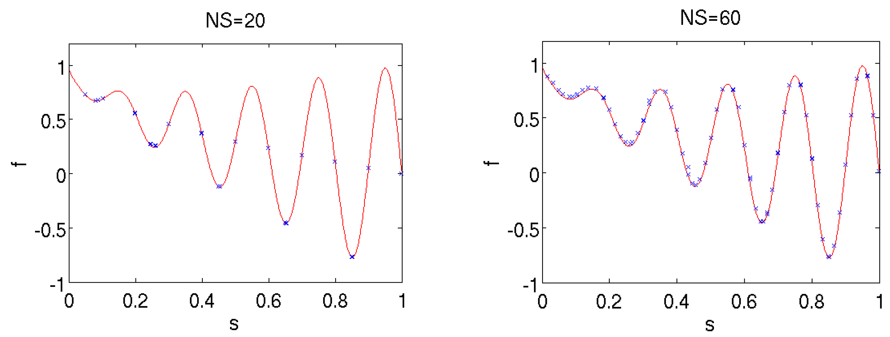
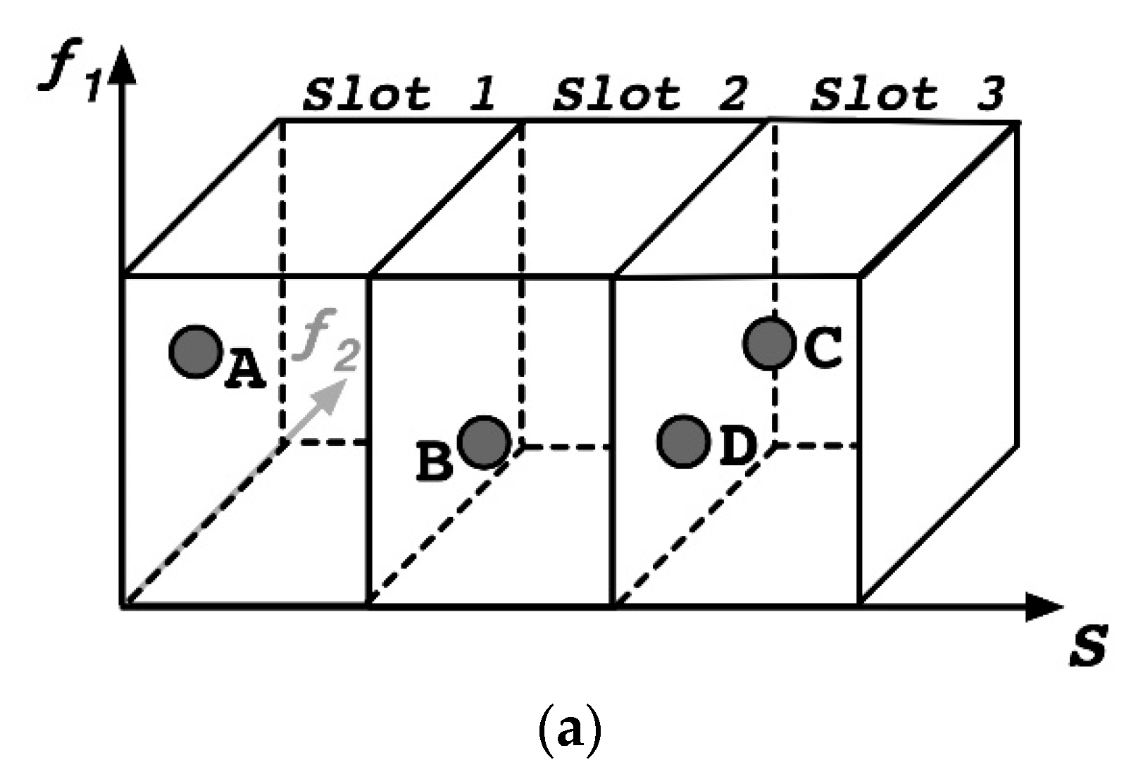
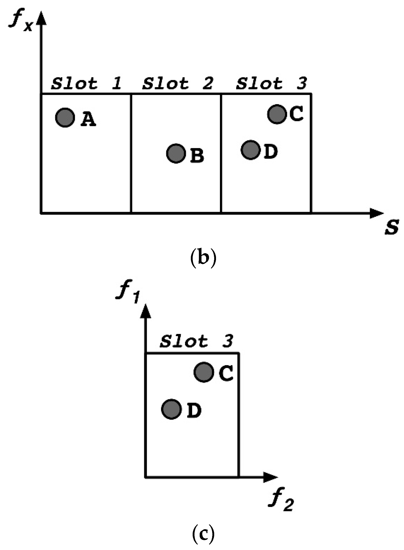
4.1. Slot-Based Sweep Dominance and Non-Dominated Sorting

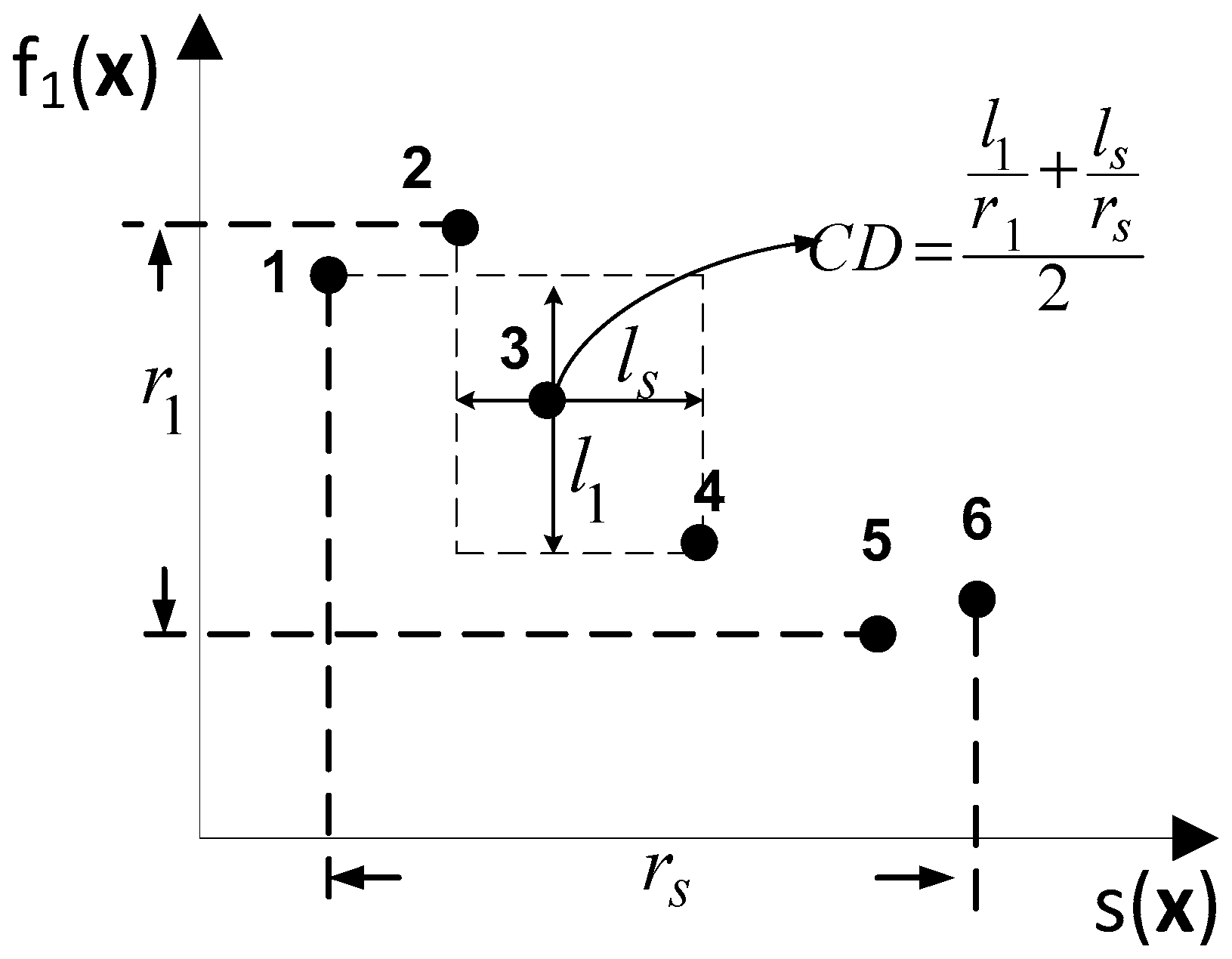
The theoretical definition of sweep dominance given above is not appropriate for our practical implementation of a solution algorithm because, with $s\left(x\right)$ being a real-valued function, the probability that two candidate solutions have the same value of $s\left(x\right)$ is extremely low. Therefore, no algorithm exploiting the sweep dominance among solutions would be effective.

Therefore, for practical implementation, a modified dominance definition is used here. Assuming that the minimum and maximum values of $s\left(x\right)$ are $S_{min}$ and $S_{max}$, respectively, and dividing the range $[S_{min},S_{max}]$ into $NS$ slots, a solution $a$ is said to sweep-dominate solution $b$ if and only if $s\left(a\right)$ and $s\left(b\right)$ belong to the same slot, $f_i\left(a\right)\le f_i\left(b\right)$ for every $i\in \left\{1,\cdots ,m\right\}$ and $f_j\left(a\right)<f_j\left(b\right)$ for at least an index$j\in \left\{1,\cdots ,m\right\}$.

Consider, for illustration purposes, the problem in Figure 5a with one sweeping objective, two minimization objectives and three slots. Solutions A and B, or B and C, are non-dominated between them because they belong to different slots of the sweeping objective $s\left(x\right)$. However, considering only solutions C and D, solution D dominates solution C because both belong to the third slot, and, as illustrated in the projection in Figure 5c, solution D is better in both objectives.

This definition can introduce a non-dominated sorting procedure similar to that in multi-objective optimization algorithms. Given a set of $N$ solutions, the set of non-constrained sweep-dominated solutions is assigned rank 1. If the solutions with rank 1 are eliminated from this set, a new set with $N\prime$ solutions is obtained. Then, the set of non-constrained sweep-dominated solutions from these $N\prime$ solutions is assigned rank 2. This process is repeated until all solutions are assigned a rank.

4.2. Diversity

In addition to the convergence toward the SPF, a good diversity of solutions is also desired. Spread must be understood here in a broad sense. Not only should the solutions have a good spread in the space of minimization objectives, but they should also extend over the broadest possible range of the sweeping objective and be uniformly distributed.

This goal can be easily accomplished by adapting existing diversity preservation mechanisms. One such mechanism uses the crowding distance (CD) [23]. The crowding distance in multi-objective optimization problems measures the density of points around each solution by averaging the distance of each such solution to the two adjacent solutions along each of the objectives. The diversity of solutions is thus preserved by maximizing the minimal crowding distance of all solutions.

The same concept can be applied to our problem by considering (only in terms of crowding distance calculation) a set of objectives $F\left(x\right)$ that involves not only the minimization objectives $f\left(x\right)$ in (3) but also the sweeping objective$s\left(x\right)$:

$$\left[F_1\left(x\right),\cdots ,F_{m+1}\left(x\right)\right]=\left[f_1\left(x\right),\cdots ,f_m\left(x\right),s\left(x\right)\right]$$

(4)

The crowding distance calculation for the new kind of optimization problem is illustrated in Figure 6 for the case of an optimization problem with one sweeping objective and one minimization objective.

4.3. Proposed Algorithm

The implementation of the algorithm is detailed in Algorithm 1.

Algorithm 1: Sweep-Pareto front calculation

Inputs: the maximum number of generations ngen, the population size N, the number of slots NS, the crossover parameter settings, the mutation parameter settings. 1: Initialization: Randomly generate an initial population of $N$ solutions $x^1,\cdots ,x^N$. Initialize current_generation = 0. 2: while (current_generation < ngen) do 3:    Offspring generation: Select pairs of parent solutions and apply the crossover and mutation operators to generate $N$ children. 4:    Update slots: Update the minimum and maximum values of the sweeping objective, $S_{min}$ and $S_{max}$, respectively, and calculate the bounds of the $NS$ slots. 5:    Ranking and selection: Rank the population, formed by merging $N$ parents and $N$ children: rank 1 for the set of non-sweep-dominated solutions of the merged set, from which they are extracted; rank 2 for the non-sweep-dominated solutions of the remaining set, and so on. Only keep $N$ solutions for the next generation. Prioritize the lowest rank solutions and larger crowding distance solutions within the same rank for selection for the next generation. 6:    Increase current_generation by 1. 7: end while 8: return approximation of the SPS: $\left\{x^1,\cdots ,x^N\right\}$ and approximation of the SPF; $\left\{F\left(x^1\right),\cdots ,F\left(x^N\right)\right\}$.

Selection in lines 3 and 5 in Algorithm 1 requires a comparison of solutions. The following rules are applied:

• If two infeasible solutions are compared, the one with the smallest constraint violation is selected.
• If one solution is feasible and the other is infeasible, the feasible one is selected.
• If two feasible solutions are compared, the one that sweep-dominates the other is selected.
• If two feasible solutions that do not sweep-dominate each other are compared, the one with a higher crowding distance is selected.

These rules ensure that feasible solutions are prioritized over infeasible ones. Then, the convergence of solutions toward the SPF is prioritized. Finally, the uniformity of solutions in the objective space is promoted in the case of non-dominated solutions.

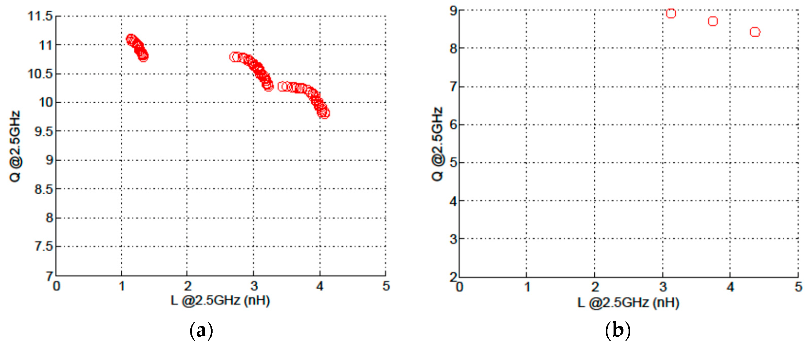
5. Experimental Results for Inductor Optimization

The proposed optimization algorithm is applied to the electronic design problem described in Section 2. In this practical application, almost all the computation time is spent evaluating the objectives and constraints. Therefore, a fair comparison with the results in Section 2, involving a similar computational effort, is made using the same number of individuals ($N=100$) and generations ($ngen=200$). The number of slots in the proposed optimization algorithm is set to $NS=80$. The optimization results are shown with blue dots in Figure 7 for the two maximum area constraints. The comparison is better visualized by superposing the plots in Figure 7 with the conventional multi-objective optimization results in Figure 4. It can be observed that the results of the proposed algorithm match the optimization results of NSGA-II in some ranges of inductance, whereas points with the maximum quality factor for other values of inductance are also obtained, as it was desired for a practical application of the results. Note that solutions with the maximum quality factor for inductance values between 0.4 nH and 1.1 nH or 1.4 nH and 2.6 nH in Figure 7a, which are impossible to obtain using a conventional optimization approach, are now attained. Similarly, solutions with a full range of inductance values are obtained in Figure 7b, with three solutions matching those in Figure 4b. Therefore, it is demonstrated that the proposed algorithm reaches the goals of the newly posed optimization problem.

Let us now consider another example with the same constraints as the previous ones (except for the area constraint, which is now $\mathrm{area}\_\max =350\times 350 {\mathsf{\mu }\mathrm{m}}^2$) and three objectives: a sweeping objective (the inductance), a maximization objective (the quality factor) and a minimization objective (the area). The execution of the algorithm, with 1000 individuals, 200 generations and 50 slots, yields the results in Figure 8. It is interesting to highlight here a specific front pattern, which is especially noticeable in the lower part of the front. This pattern is due to the number of turns of inductors, which can only take integer values. On the other hand, it can be seen that there is still a discontinuous pattern of the front in the other dimensions since the area and quality factor trade off in the conventional Pareto sense.

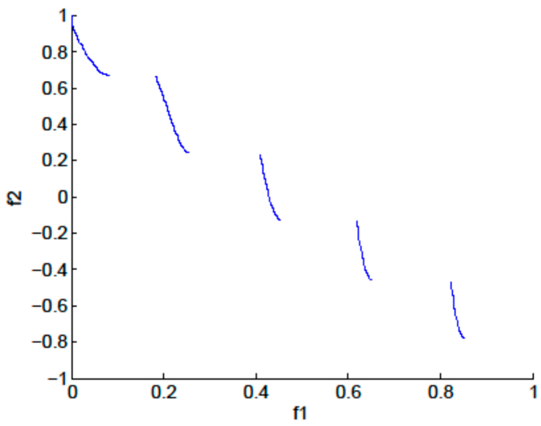
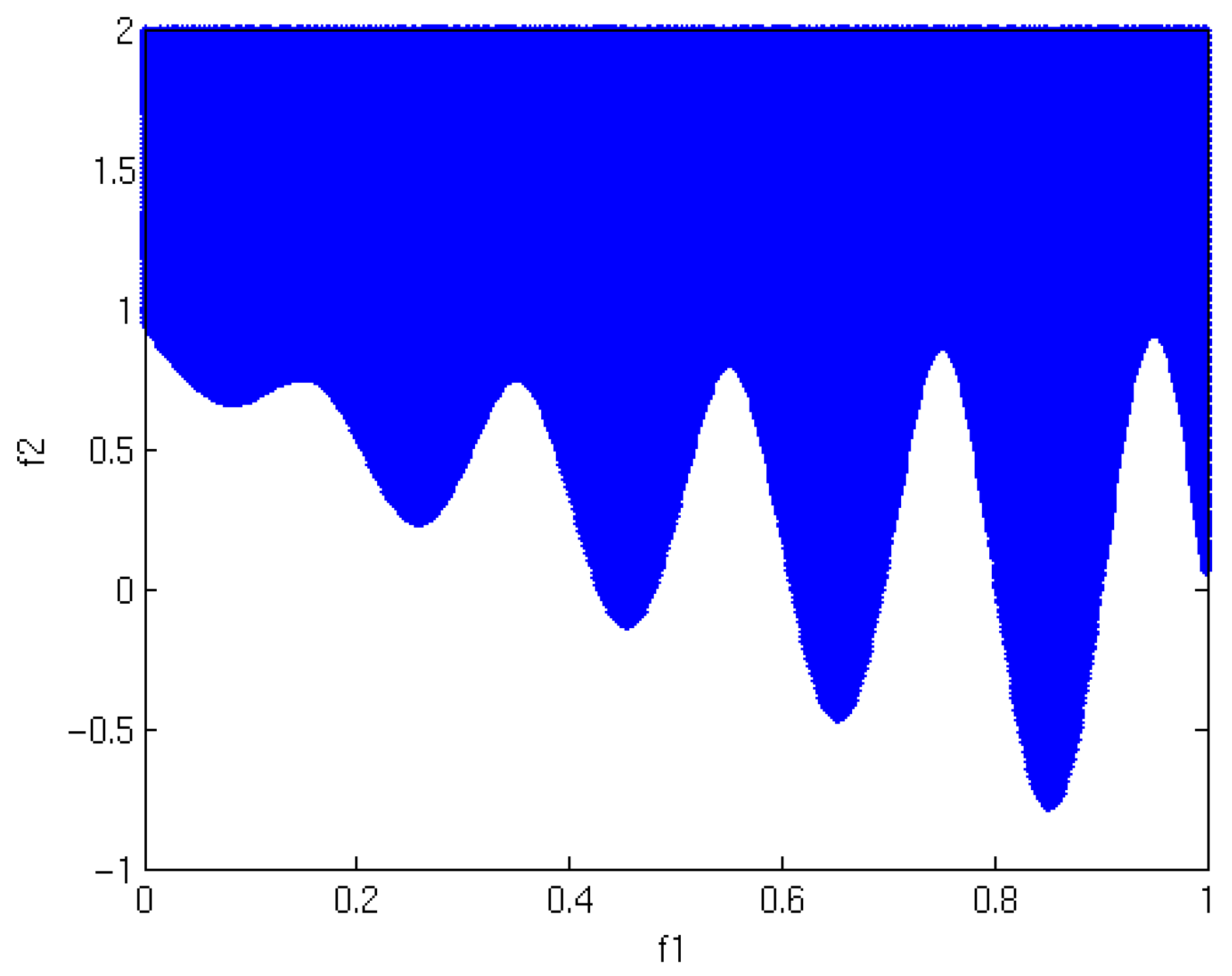
6. Mathematical Benchmark Problem

The beneficial interest of the new optimization problem was previously stated. A new algorithm was proposed, and its ability to solve this practical problem was demonstrated. However, it is clear that the examples above are only accessible to specialists in the field. It is also important to have some mathematical benchmark functions with similar characteristics that can ease algorithm development by non-specialists. In this Section, such a mathematical function is used, and the proposed algorithm is extensively tested with this example.

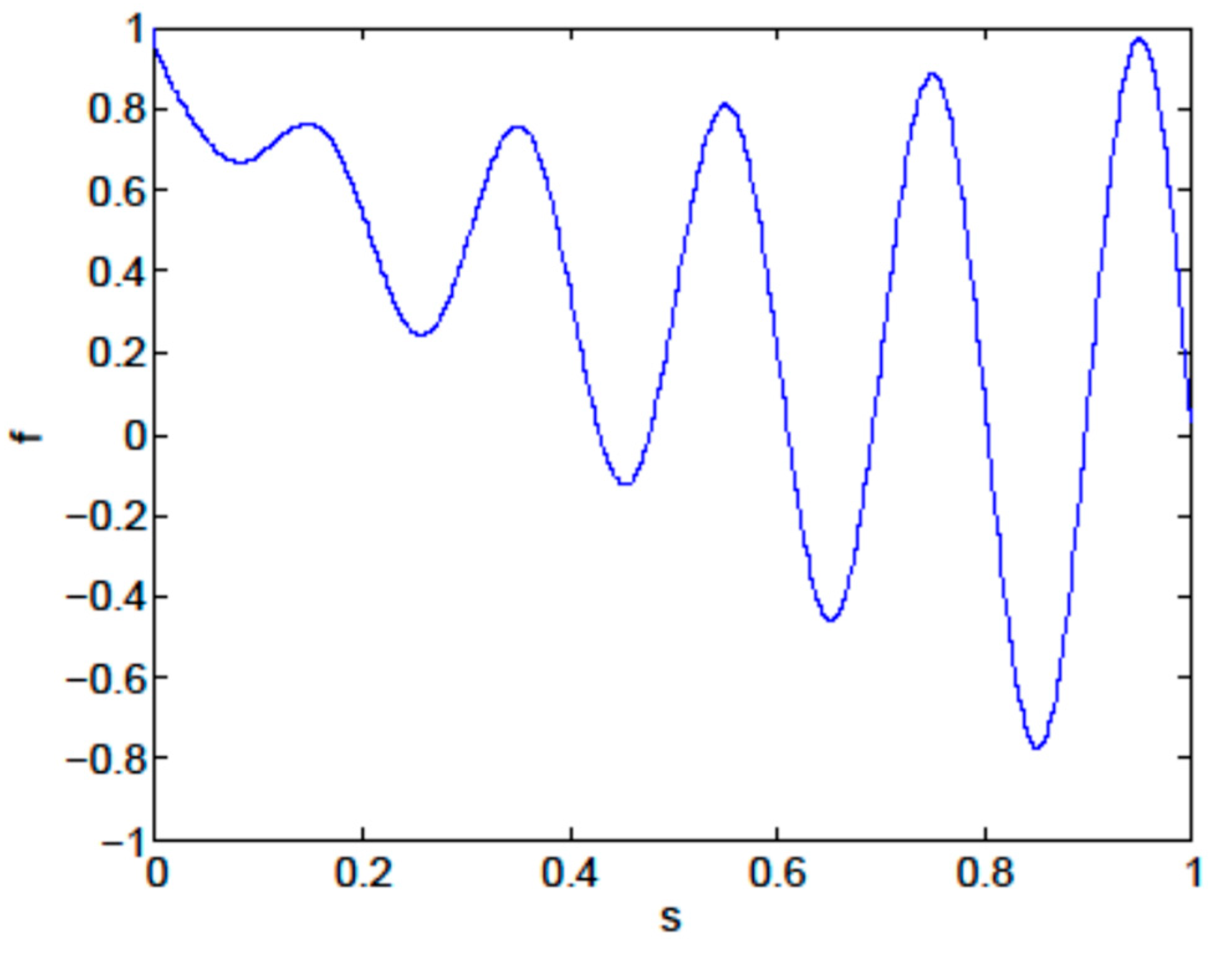
6.1. Mathematical Benchmark Function

There is no mathematical benchmark problem specifically defined to develop, test and compare this optimization algorithm, as this type of problem has not been reported before. However, some existing benchmarks for conventional multi-objective optimization problems, whose solution is a discontinuous Pareto front, can be easily adapted to the optimization problem reported here. Let us consider, for instance, the conventional minimization formulation of problem ZDT3 defined in a 30-dimensional (n = 30) search space as follows [28]:

$$\mathrm{minimize} \left\{\begin{array}{cc}\begin{array}{c}{f}_1\left(x\right)=x_1\\ f_2\left(x\right)=g\left(x\right)·h\left(f_1\left(x\right),g\left(x\right)\right)\end{array}& 0\le x_i\le 1\end{array}\right.$$

(5)

where

$$h\left(f_1\left(x\right),g\left(x\right)\right)=1-\sqrt{f_1\left(x\right)/g\left(x\right)}-\left(f_1\left(x\right)/g\left(x\right)\right)\sin \left(10\pi f_1\left(x\right)\right)$$

(6)

and

$$g\left(x\right)=1+\frac{9}{n-1}{\displaystyle \sum }_{i=2}^n{x}_i.$$

(7)

The graphical representation of the most interesting region of the objective functions is shown in Figure 9, where the possible objective function values that the solutions can take are shaded in blue. The true Pareto front of the minimization problem shown in Equation (5) is given by

$$(f_1,1-\sqrt{f_1}-f_1\sin \left(10\pi f_1\right))$$

(8)

with$f_1$:

$$\begin{array}{ll}{f}_1\in \left[0.0, 0.083001\right]& \cup \left(0.182228, 0.257762\right]\cup \left(0.409313, 0.453882\right]\\ & \cup \left(0.618396, 0.652511\right]\cup \left(0.823331, 0.851832\right]\end{array}$$

(9)

and is plotted in Figure 10.

A sweeping multi-objective problem can be easily derived from Equation (5) as follows:

$$\begin{array}{cc}\begin{array}{c}\mathrm{sweep} s\left(x\right)=x_1\\ \mathrm{minimize}f\left(x\right)=g\left(x\right)·h\left(s\left(x\right),g\left(x\right)\right)\end{array}& 0\le x_i\le 1\end{array}$$

(10)

where $g(x)$ and $h(x)$ are defined as in (6) and (7). The sweep-Pareto front is given by

$$(s,1-\sqrt{s}-s·\sin \left(10\pi s\right))$$

(11)

with$s$:

$$s\in \left[0.0,1.0\right]$$

(12)

This front is plotted in Figure 11.

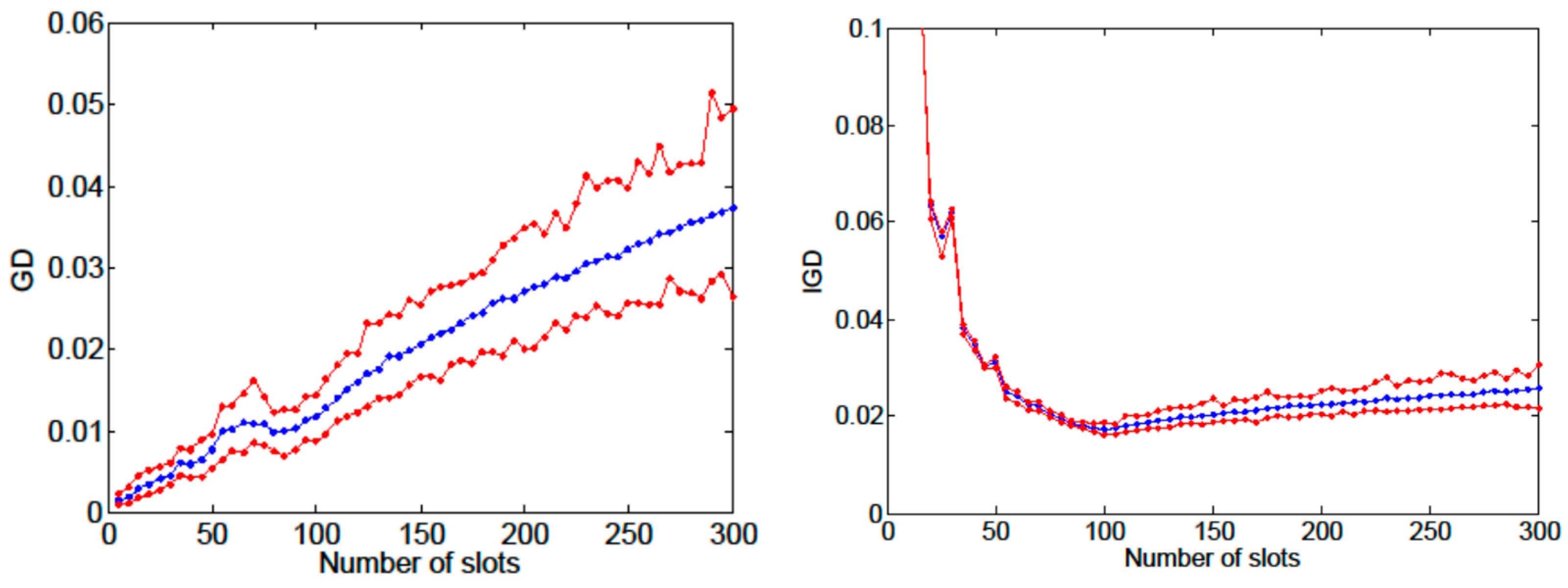
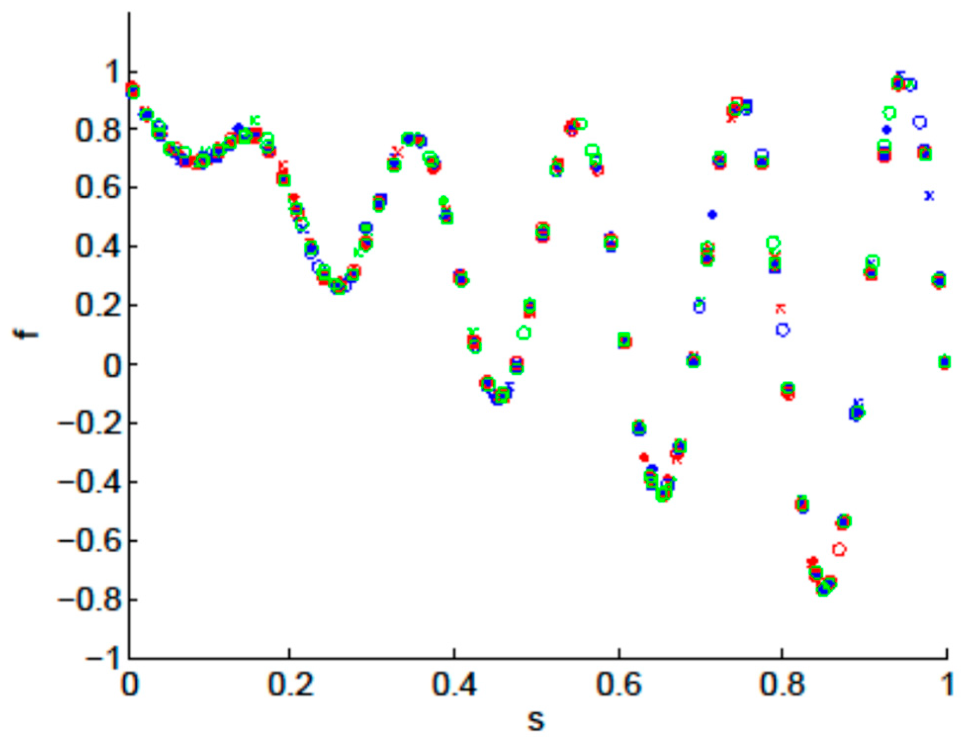
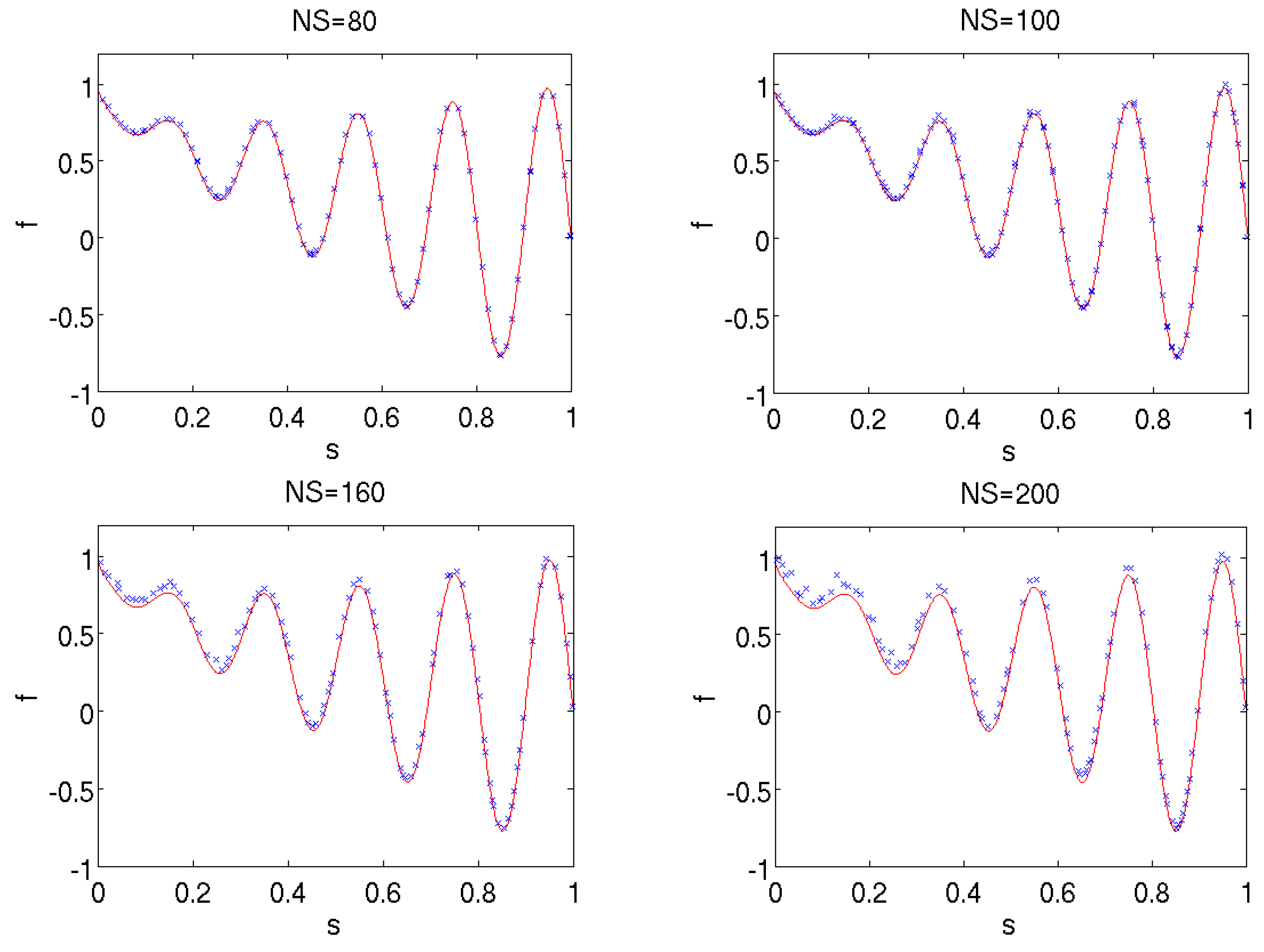
6.2. Experimental Results

The algorithm proposed in Section 4 was applied to the mathematical benchmark problem described above using a population of 100 individuals along 200 generations. The results of nine different executions are shown in Figure 12. It can be clearly seen that the algorithm consistently provides good approximations of the desired SPF.

As detailed in Section 4, one configuration parameter is the number of slots, $NS$. It is important to investigate the influence of this parameter on the quality of the results. Therefore, the same experiment was executed with six different settings of the $NS$ parameter. The results, together with the true SPF, can be seen in Figure 13. It appears that selecting a value of $NS$ that is too low negatively impacts the density and diversity of points, whereas selecting a value that is too high can affect the convergence.

However, this experiment has two limitations. First, being a stochastic optimization algorithm, no conclusion should be drawn from a single execution of a given parameter setting. Second, some performance metrics for the evaluation of the quality of the fronts, beyond a visual inspection of the results, should be used. Even though performance metrics were developed to test and compare conventional multi-objective optimization algorithms, some of them can be easily adapted to the optimization problem proposed here.

A standard metric in multi-objective optimization is the generational distance (GD) [29], defined as the average distance between each solution in an approximation to the Pareto front $P{F}^{ap}$ and the closest solution in the reference (true) Pareto front $P{F}^{true}$:

$$GD\left(P{F}^{ap}\right)=\frac{{{\displaystyle \sum }}_{v\in P{F}^{ap}}\underset{r\in P{F}^{true}}{\min }d\left(v,r\right)}{\left|P{F}^{ap}\right|}$$

(13)

where $d\left(v,r\right)$ is usually associated with the Euclidean distance between solutions $v$ and $r$ in the objective space, although other distance definitions have been reported [30]. The Euclidean distance commonly uses normalized objective function values to avoid the bias of disparately scaled objectives. The generational distance correlates well with convergence to the reference set. However, good $GD$ values may be obtained by Pareto fronts with poor diversity. In particular, for the proposed problem in Equation (10), it is interesting that the solutions have an excellent convergence to the true SPF for each specific value of the sweeping objective $s\left(x\right)$. Therefore, we propose a modified distance definition for the $GD$ calculation in the optimization problem in Equation (10):

$$d\left(v,r\right)=\left\{\begin{array}{cc}\sqrt{{\displaystyle {\displaystyle \sum }_{k=1}^n}{\left(v_k-r_k\right)}^2}& \mathrm{if} v_s=r_s\\ \infty & \mathrm{otherwise}\end{array}\right.$$

(14)

where $v_s$ and $r_s$ denote the sweeping objective coordinate of solutions $v$ and $r$, respectively, and $v_k$ and $r_k$ denote the k-th minimization objective coordinate of the same solutions. With this distance calculation, Equation (13) refers to the average distance between each solution to the closest solution in the true SPF subset with the same value of the sweeping objective. Such average distance can be easily calculated in problems such as Equation (10), as the points of the true SPF are known for any value of the sweeping objective (given by Equation (11) for the problem in Equation (10)).

Another popular metric is the inverted generational distance, defined as follows [31]:

$$IGD\left(P{F}^{ap}\right)=\frac{{{\displaystyle \sum }}_{v\in P{F}^{true}}\underset{r\in P{F}^{ap}}{\min }d\left(v,r\right)}{\left|P{F}^{true}\right|}$$

(15)

where $\underset{r\in P{F}^{ap}}{\min }d\left(v,r\right)$ is the Euclidean distance between each reference point $v$ of a selected set of the true Pareto front $P{F}^{true}$ and the closest solution $r$ of the approximated Pareto front$P{F}^{ap}$. As with $GD$, the Euclidean distance uses normalized objective function values. A low value of $IGD$ implies that the points of $P{F}^{ap}$ are sufficiently close to the true PF and cover a wide spread of it; i.e., it measures a balance of convergence and diversity. This definition directly applies to our problem by only replacing each Pareto front (PF) with the sweep-Pareto front (SPF).

Once the performance metrics are defined, a statistical study can be performed to assess the influence of the $NS$ parameter. Therefore, the experiment was repeated using 60 different settings of $NS$ equally spaced between 5 and 300. The proposed optimization algorithm was executed 100 times for each of these settings, and both $GD$ and $IGD$ were calculated. The $IGD$ values are known to depend on the selection of the reference points [32]. For the $IGD$ calculation, a subset of the true SPF with 1000 points uniformly distributed along the sweeping objective was used. The mean values of $GD$ and $IGD$ vs. the number of slots $NS$ are plotted in blue in Figure 14. The upper and lower red plots correspond to the $GD$ and $IGD$ values of the best and worst execution. It can be seen that the generational distance is better for small values of the number of slots. This result can be explained by the fact that the available solutions in the approximated SPF converged reasonably close to the true SPF, which is consistent with the results obtained in Figure 13. However, this metric does not consider the diversity of solutions along the front. Looking at the inverted generational distance, we can see that the best value is obtained for around 100 slots and increases slightly for larger values. This result is also consistent with the results in Figure 13, as the worst convergence for a higher number of slots is compensated by an improved diversity. It can be concluded, therefore, that, for this benchmark problem with two objectives, the number of slots should be set slightly below or above the population size, depending on the preference for either stressing convergence or diversity.

7. Conclusions

This paper presented a new type of multi-objective optimization problem motivated by real-world practical applications, particularly the multi-objective optimization of integrated inductors. The problem was mathematically formulated, and a solution algorithm was proposed. A mathematical benchmark problem was also proposed to enable the development and comparison of optimization algorithms.

References

1. Rutenbar, R.; Gielen, G.; Roychowdhury, J. Hierarchical modeling, optimization and synthesis for system-level analog and RF designs. Proc. IEEE 2007, 95, 640–669. [Google Scholar] [CrossRef]
2. Alpaydin, G.; Balkir, S.; Dundar, G. An evolutionary approach to automatic synthesis of high-performance analog integrated circuits. IEEE Trans. Evol. Comput. 2003, 7, 240–252. [Google Scholar] [CrossRef]
3. Liu, B.; Fernandez, F.V.; Gielen, G. Efficient and accurate statistical analog yield optimization and variation-aware circuit sizing based on computational intelligence techniques. IEEE Trans. Comput.-Aided Des. Integr. Circuits Syst. 2011, 30, 793–805. [Google Scholar] [CrossRef]
4. Lourenço, N.; Martins, R.; Horta, N. Automatic Analog IC Sizing and Optimization Constrained with PVT Corners and Layout Effects; Springer: Cham, Switzerland, 2017. [Google Scholar] [CrossRef]
5. Liu, B.; Gielen, G.; Fernandez, F.V. Automated Design of Analog and High-Frequency Circuits. A Computational Intelligence Approach; Springer: Berlin/Heidelberg, Germany, 2014. [Google Scholar] [CrossRef]
6. Hussain, A.; Kim, H.-M. Evaluation of Multi-Objective Optimization Techniques for Resilience Enhancement of Electric Vehicles. Electronics 2021, 10, 3030. [Google Scholar] [CrossRef]
7. Stehr, G.; Graeb, H.; Antreich, K. Analog performance space exploration by normal-boundary intersection and by Fourier-Motzkin elimination. IEEE Trans. Comput.-Aided Des. Integr. Circuits Syst. 2007, 26, 1733–1748. [Google Scholar] [CrossRef]
8. Liu, B.; Zhang, Q.; Fernandez, F.V.; Gielen, G. An efficient evolutionary algorithm for chance-constrained bi-objective stochastic optimization. IEEE Trans. Evol. Comput. 2013, 17, 786–796. [Google Scholar] [CrossRef]
9. Eeckelaert, T.; McConaghy, T.; Gielen, G. Efficient multiobjective synthesis of analog circuits using hierarchical Pareto-optimal performance hypersurfaces. In Proceedings of the Design, Automation and Test in Europe Conference, Munich, Germany, 7–11 March 2005; Volume 2, pp. 1070–1075. [Google Scholar] [CrossRef]
10. Gonzalez-Echevarria, R.; Castro-López, R.; Roca, E.; Fernández, F.V.; Sieiro, J.; Vidal, N.; López-Villegas, J.M. Automated generation of the optimal performance trade-offs of integrated inductors. IEEE Trans. Comput.-Aided Des. Integr. Circuits Syst. 2014, 33, 1269–1273. [Google Scholar] [CrossRef]
11. Passos, F.; Roca, E.; Castro-Lopez, R.; Fernandez, F.V. Radio-frequency inductor synthesis using evolutionary computation and Gaussian process surrogate modeling. Appl. Soft Comput. 2017, 60, 495–507. [Google Scholar] [CrossRef]
12. Gonzalez-Echevarria, R.; Roca, E.; Castro-López, R.; Fernández, F.V.; Sieiro, J.; López-Villegas, J.M.; Vidal, N. An automated design methodology of RF circuits by using pareto-optimal fronts of EM-simulated inductors. IEEE Trans. Comput.-Aided Des. Integr. Circuits Syst. 2017, 36, 15–26. [Google Scholar] [CrossRef]
13. Passos, F.; Roca, E.; Sieiro, J.; Fiorelli, R.; Castro-López, R.; López-Villegas, J.M.; Fernández, F.V. A Multilevel Bottom-Up Optimization Methodology for the Automated Synthesis of RF Systems. IEEE Trans. Comput.-Aided Des. Integr. Circuits Syst. 2020, 39, 560–571. [Google Scholar] [CrossRef]
14. Kotti, M.; Gonzalez-Echevarria, R.; Fernández, F.V.; Roca, E.; Sieiro, J.; Castro-López, R.; Fakhfakh, M.; López-Villegas, J.M. Generation of surrogate models of Pareto-optimal performance trade-offs of planar inductors. Analog. Integr. Circuits Signal Processing 2014, 78, 87–97. [Google Scholar] [CrossRef]
15. Passos, F.; Roca, E.; Castro-Lopez, R.; Fernandez, F.V. An algorithm for a class of real-life multi-objective optimization problems with a sweeping objective. In Proceedings of the IEEE Congress on Evolutionary Computation, Donostia, Spain, 5–8 June 2017; pp. 737–740. [Google Scholar] [CrossRef]
16. Deb, K. An efficient constraint handling method for genetic algorithms. Comput. Methods Appl. Mech. Eng. 2000, 186, 311–338. [Google Scholar] [CrossRef]
17. Jan, M.A.; Zhang, Q. MOEA/D for constrained multiobjective optimization: Some preliminary experimental results. In Proceedings of the UK Workshop on Computational Intelligence, Colchester, UK, 8–10 September 2010. [Google Scholar] [CrossRef]
18. Asafuddoula, M.; Ray, T.; Sarker, R.; Alam, K. An adaptive constraint handling approach embedded MOEA/D. In Proceedings of the IEEE Congress on Evolutionary Computation, Brisbane, QLD, Australia, 10–15 June 2012. [Google Scholar] [CrossRef]
19. Zapotecas Martinez, S.; Coello, C.A. A multi-objective evolutionary algorithm based on decomposition for constrained multi-objective optimization. In Proceedings of the IEEE Congress on Evolutionary Computation, Beijing, China, 6–11 July 2014. [Google Scholar] [CrossRef]
20. Jan, M.A.; Khanum, R.A. A study of two penalty-parameterless constraint handling techniques in the framework of MOEA/D. Appl. Soft Comput. 2013, 13, 128–148. [Google Scholar] [CrossRef]
21. Lopez-Villegas, J.M.; Samitier, J.; Cane, C.; Losantos, P.; Bausells, J. Improvement of the quality factor of RF integrated inductors by layout optimization. IEEE Trans. Microw. Theory Tech. 2000, 48, 76–83. [Google Scholar] [CrossRef]
22. Chen, H.-H.; Hsu, Y.-W. Analytic Design of on-Chip Spiral Inductor with Variable Line Width. Electronics 2022, 11, 2029. [Google Scholar] [CrossRef]
23. Deb, K.; Pratap, A.; Agarwal, S.; Meyarivan, T. A fast and elitist multiobjective genetic algorithm: NSGA-II. IEEE Trans. Evol. Comput. 2002, 6, 182–197. [Google Scholar] [CrossRef]
24. Zhang, Q.; Li, H. MOEA/D: A multiobjective evolutionary algorithm based on decomposition. IEEE Trans. Evol. Comput. 2007, 11, 71–731. [Google Scholar] [CrossRef]
25. Hua, Y.; Jin, Y.; Hao, K. A clustering-based adaptive evolutionary algorithm for multiobjective optimization with irregular Pareto fronts. IEEE Trans. Cybern. 2019, 49, 2758–2770. [Google Scholar] [CrossRef]
26. Jiang, S.; Yang, S. An improved multiobjective optimization evolutionary algorithm based on decomposition for complex Pareto fronts. IEEE Trans. Cybern. 2016, 46, 421–437. [Google Scholar] [CrossRef]
27. Deb, K. Multi-Objective Optimization Using Evolutionary Algorithms; Wiley: Hoboken, NJ, USA, 2001. [Google Scholar]
28. Zitzler, E.; Deb, K.; Thiele, L. Comparison of multiobjective evolutionary algorithms: Empirical results. Evol. Comput. 2000, 8, 173–195. [Google Scholar] [CrossRef]
29. Van Veldhuizen, D.A. Multiobjective Evolutionary Algorithms: Classifications, Analyzes, and New Innovations. Ph.D. Dissertation, Graduate School of Engineering of the Air Force Institute of Technology, Air University, Fairborn, OH, USA, June 1999. [Google Scholar]
30. Bezerra, L.C.; Lopez-Ibañez, M.; Stutzle, T. An empirical assessment of the properties of inverted generational distance on multi- and many-objective optimization. In Proceedings of the 9th International Conference on Evolutionary Multi-Criterion Optimization, Muenster, Germany, 19–22 March 2017; pp. 31–45. [Google Scholar] [CrossRef]
31. Zitzler, E.; Thiele, L.; Laumanns, M.; Fonseca, C.; da Fonseca, V. Performance assessment of multi-objective optimizers: An analysis and review. IEEE Trans. Evol. Comput. 2003, 7, 117–132. [Google Scholar] [CrossRef]
32. Ishibushi, H.; Masuda, H.; Tanigaki, Y.; Nojima, Y. Difficulties in specifying reference points to calculate the inverted generational distance for many-objective optimization problems. In Proceedings of the IEEE Symposium Computational Intelligence in Multi-Criteria Decision-Making, Orlando, FL, USA, 9–12 December 2014; pp. 170–177. [Google Scholar] [CrossRef]
Figure 1. Illustrating bottom-up Pareto-front composition.
Electronics 11 02624 g001
Figure 2. Geometric parameters of an octagonal asymmetric spiral inductor. Different color stripes correspond to different metal layers.
Electronics 11 02624 g002
Figure 3. Illustrating the inductance and quality factor as a function of frequency for three different inductors.
Electronics 11 02624 g003
Figure 4. Resulting Pareto front from the maximization of inductance and quality factor with maximum area constraint (a) area_max = 200 × 200   μ m 2 and (b) area_max = 100 × 100   μ m 2 .
Electronics 11 02624 g004
Figure 5. (a) Objective space with two minimization objectives f1 and f2 and one sweeping objective s; (b) projection in fxs plane; (c) projection in the f1f2 plane.
Electronics 11 02624 g005aElectronics 11 02624 g005b
Figure 6. Illustration of the crowding distance calculation of one solution for the optimization problem with one minimization objective and one sweeping objective.
Electronics 11 02624 g006
Figure 7. Sweep-Pareto fronts (blue dots) with inductance as sweeping objective and maximization of quality factor with maximum area constraint: (a) area_max = 200 × 200   μ m 2 and (b) area_max = 100 × 100   μ m 2 . Pareto fronts obtained in Figure 4 with conventional multi-objective optimization are superimposed with red circles to ease the comparison.
Electronics 11 02624 g007
Figure 8. Sweep-Pareto front with inductance as sweeping objective and maximization of quality factor and minimization of area.
Electronics 11 02624 g008
Figure 9. The objective space for problem ZDT3.
Electronics 11 02624 g009
Figure 10. True Pareto front for the optimization problem in Equation (5).
Electronics 11 02624 g010
Figure 11. True sweep-Pareto front for the optimization problem in Equation (10).
Electronics 11 02624 g011
Figure 12. Sweep-Pareto fronts obtained with nine executions (each shown with different symbol and/or color) of the proposed algorithm on the problem in Equation (10).
Electronics 11 02624 g012
Figure 13. Optimization results on the proposed mathematical benchmark problem for six different settings of the NS parameter. The true SPF is plotted with a continuous red line.
Electronics 11 02624 g013aElectronics 11 02624 g013b
Figure 14. Generational distance (GD) and inverted generational distance (IGD) vs. the number of slots for the optimization problem in Equation (10). Blue dots correspond to the mean values of 100 executions. Upper and lower red dots correspond to the worst and best executions.
Electronics 11 02624 g014