Built-In Functional Testing of Analog In-Memory Accelerators for Deep Neural Networks

Abstract

The paper develops a methodology for the online built-in self-testing of deep neural network (DNN) accelerators to validate the correct operation with respect to their functional specifications. The DNN of interest is realized in the hardware to perform in-memory computing using non-volatile memory cells as computational units. Assuming a functional fault model, we develop methods to generate pseudorandom and structured test patterns to detect hardware faults. We also develop a test-sequencing strategy that combines these different classes of tests to achieve high fault coverage. The testing methodology is applied to a broad class of DNNs trained to classify images from the MNIST, Fashion-MNIST, and CIFAR-10 datasets. The goal is to expose hardware faults which may lead to the incorrect classification of images. We achieve an average fault coverage of 94% for these different architectures, some of which are large and complex.

1. Introduction

Deep neural networks (DNNs) are pervasive in artificial intelligence applications involving computer vision, image processing, speech recognition, and robotics. When deployed on resource-constrained edge devices, the DNN model performs inference on a continuous basis to analyze the information gathered from its operating environment—consuming a considerable amount of energy in this process. Therefore, high-performance yet low-power operation is a critical requirement.

In-memory computing using non-volatile memory (NVM) cells as computational units can provide significant power and speed benefits for machine-learning inference tasks. Crossbar-based architectures are typical, consisting of an array of n rows by n columns with NVM-based storage elements located at their crosspoints [1,2]. Synaptic weights are specified in terms of the conductivity of the NVM cells, allowing these cells to act as computational units through the analog summation of the current that flows through them.

The NVM device of a synaptic cell can be implemented using technologies such as phase-change memory (PCM), oxide-based memory (OxRAM), and spin-based magnetic memory (STT-MRAM) [1,3,4]. High voltages, generated via on-chip charge pumps built using CMOS devices, are required to read or to program these NVM cells. High-voltage operations, unfortunately, have negative consequences for hardware reliability. Common issues include higher NVM-cell wear-out, increasing the risk of stuck-SET and stuck-RESET faults; higher resistance drift, leading to data integrity issues; and the accelerated aging of the peripheral CMOS circuits, resulting in read disturbance issues [5]. Faults affecting synaptic cells that result in erroneous values being used during inference can lead to incorrect results. For example, if the underlying DNN model performs image classification, these errors may result in more images being misclassified, which is problematic in autonomous driving or surveillance applications.

Structural and functional testing methods have been recently developed for accelerators built using systolic-array architectures [6,7]. By contrast, this paper develops testing methods aimed at exposing faults in NVM cells situated in crossbar architectures. Because the crossbar structure is similar to that of traditional RAM, test-pattern generation techniques such as March tests can be adapted to test for faults [8]. A common theme is to program a target conductance value into every NVM cell and then measure variations in the conductance when reading back [9,10,11,12]. Fault models include stuck-at and transition faults and others based on NVM’s physical characteristics, for example, a read disturbance fault, which may occur when a read current is applied during read operations but may also bias the conductance of the cell [9].

Though suitable for production testing, using any of the above methods for the field testing of crossbars presents significant practical limitations, especially when the trained machine-learning model is deployed on an edge device. This is because the following steps must be performed in sequence: (1) the inference operation must be stopped to offload the model parameters from the crossbars, (2) test patterns must be loaded to detect stuck faults, (3) preventive measures may be necessary to avoid using the faulty cells, and (4) model parameters must be reloaded on to the crossbars to continue the inference operations. Due to the limited storage capacity on edge devices, model parameters cannot be stored on the device temporarily during testing. Additionally, the offloading and reloading of the model parameters can incur a significant amount of time, during which the crossbars cannot perform any inference. The novelty of our testing methodology is that the generated test patterns are specific to the model being deployed on the crossbars. This way, model parameters need not be offloaded for testing purposes. These model-specific pseudorandom test patterns can be generated on demand, further lowering the storage requirements.

We develop a methodology for the online built-in functional testing of NVM-based in-memory accelerators for DNNs used in image classification tasks. The goal is to validate the correct operation of the DNN under test (DUT) with respect to its functional specifications by exposing faults affecting the crossbar that may cause the misclassification of the input images. This paper makes the following contributions:

• We develop test-pattern generation (TPG) methods which generate pseudorandom tests in the form of images whose pixel values are chosen from both normal and uniform distributions. The distributions themselves are created using the statistical properties of the information present within the training dataset for the DNN, and so, tests generated using these distributions are able to better sensitize weights within the DUT and achieve good fault coverage.
• Convolutional layers extract features in the form of edges and contours for the subsequent fully connected hidden layers within DNNs. Based on this observation, we develop TPG methods to generate structured patterns which mimic such features and show that these can augment pseudorandom tests to further improve the fault coverage in convolutional neural networks.
• For DNNs trained to classify color images, we develop a TPG method which uses template images to capture the underlying chrominance information and applies geometric transformations to these templates to create diversified tests.
• Output responses from the DNN for a series of test patterns are observed in the form of one-hot-encoded predicted labels. These are compressed into a signature which can be compared to a reference to detect faults.

To the best of our knowledge, ours is the first approach to use concepts from pseudorandom testing for the built-in self test of DNNs. The developed TPG methods are agnostic to the specific technology used to implement the NVM cell. These methods are integrated into a built-in self-test (BIST) scheme which aims for a small test-set size while achieving high fault coverage.

We demonstrate the broad applicability of the developed BIST scheme using some representative DNNs which are suitable for deployment on edge devices. First, we consider networks in the form of a three-layer artificial neural network (ANN), a two-layer convolutional neural network (CNN), and LeNet [13], which are trained to classify grayscale images from the MNIST and Fashion-MNIST (FMNIST) datasets. We show an average fault coverage of 95.47% for these networks. Then, using realizations of AlexNet [14] and ResNet-18 (residual network) [15] which are trained to classify color images from CIFAR-10, we show an average coverage of 87.28% for these large, more complex architectures.

The paper is organized as follows. Section 2 familiarizes the reader with the system architecture and associated reliability concerns, as well as the concept of functional testing. Section 3 develops the DNN and the associated fault models. The technical approach is developed in Section 4 and Section 5. The performance of the BIST scheme is discussed in Section 6 and Section 8. The error detection using a signature analysis on the test responses is discussed in Section 7. We discuss the related work in Section 9 and conclude the paper in Section 10.

2. Preliminaries

We describe the crossbar-based system architecture which uses NVM cells as storage elements. The various reliability concerns associated with popular NVM technologies are also discussed.

2.1. System Architecture

The DNN of interest is mapped onto a tile-based architecture in which each tile consists of a crossbar array and communicates with other tiles via a network interconnect. Each crossbar is an array of n rows by n columns with NVM-based storage elements located at the crosspoints. Figure 1 shows a 3D view of a crossbar in terms of the top electrodes (TEs) which form rows and the bottom electrodes (BEs) which form columns. A synaptic cell is connected at a crosspoint via an access transistor. The NVM is shown as a resistive element. The pre-synaptic neurons are mapped along the TEs and post-synaptic neurons along the BEs. The synaptic weight between a pre- and a post-synaptic neuron is programmed as the conductance of the corresponding synaptic cell at the crosspoint. A pre-synaptic neuron’s voltage v, applied on the TE, is multiplied by the conductance to generate a current according to Ohm’s Law. The current summation occurs on each BE according to Kirchoff’s Current Law, when integrating excitation from other pre-synaptic neurons. The figure shows the integration of the input excitation from two pre-synaptic neurons to one post-synaptic neuron via synaptic weights $w_1$ and $w_2$, respectively. The current summations along the column implement the multiply and accumulate operation, $w_1{v}_1+w_2{v}_2$, needed for the forward propagation of neuron activation.

Take, for example, the PCM-based cell shown in Figure 1 which is built using a chalcogenide semiconductor alloy called GST in whose amorphous phase exhibits higher resistance than the crystalline phase [1]. To compute $w_i{v}_i$, a controlled current is injected into the resistor–chalcogenide junction via the heater element to ensure that the phase of the PCM cell is not disturbed. This is the fundamental operation of the forward propagation of neuron excitation during inference. To program or update a synaptic weight, the injected current is controlled to heat the GST, thereby changing its conductivity. The current practice is to set voltages of 5.7 V for SET (0 → 1), 13.1 V for RESET (1 → 0), and 3.85 V to read the weights. These voltages are generated using an on-chip charge pump.

Each NVM cell can be programmed to a low-resistance state (LRS) or a high-resistance state (HRS) by appropriately setting its conductance. To represent multiple bits per cell, an intermediate LRS can be programmed into the cell [1]. To implement two bits per cell, for instance, it can be programmed for one HRS to represent zero or one of three different LRSs to represent non-zero values.

2.2. Reliability Issues

To read or to program an NVM cell, a peripheral circuit drives the current through it using a bias voltage which must be high enough to compensate for both the ohmic potential drop and the built-in potential of the access device which connects the cell to a row and a column in the crossbar [1,16]. Therefore, high-voltage operations are common in crossbar architectures with PCM, FeRAM, and Flash NVMs, and these voltages are generated via on-chip charge pumps built using CMOS devices. High-voltage operations lower the NVM cell reliability. Common issues include higher wear-out and increasing the risk of stuck-at-SET and stuck-at-RESET faults; higher resistance drift leading to data integrity issues; higher electro-migration in the metal contacts leading to cell lifetime issues; and higher probability of threshold switching during read operations resulting in read disturbance issues.

High-voltage operations also cause aging of the access transistor in each synaptic cell in a crossbar and also of the transistors in each neuron connected along the TEs and the BEs of the crossbar [17]. Aging accelerates when the transistor is exposed to a high overdrive voltage, defined as the voltage between the transistor gate and the source in excess of the threshold voltage which is the minimum voltage required between the gate and the source to turn the transistor on. The failure mechanisms include the Time-Dependent Dielectric Breakdown, Bias Temperature Instability, and Hot-Carrier Injection [5]. Referring back to Figure 1, these failure mechanisms may cause the access transistor to be stuck at 0/1 or to switch incorrectly when reading from/writing to NVM cells.

Aging-induced defects differ from endurance failures, which are due to the repeated programming of NVM cells [18]. Aging-related issues arise during inference (reading of synaptic weights) and training (update of synaptic weights) in supervised machine learning, while endurance issues arise only during training [19].

3. Neural Network and Fault Modeling

Full-precision DNNs that use 32-bit floating-point values to hold synaptic weights are not suitable for deployment on edge device due to high computational and memory costs. Therefore, starting with a full-precision model, we use an existing state-of-the-art approach to prune and quantize the DNN, aiming to compress the model and to speed up inference [20,21].

From the viewpoint of applying BIST, a well-trained compressed model makes it easier to achieve good fault coverage using fewer tests. This is because there are fewer weights to test, and because pruning removes less salient weights that minimally impact the network’s accuracy, the surviving weights are now quite sensitive to changes caused by stuck-at-SET and stuck-at-RESET faults in the hardware, and therefore are easier to sensitize using the pseudorandom tests.

3.1. Compressing the DNN Architecture

Figure 2 shows the design flow to obtain a compressed ternary-weight version of the original DNN which contains one of only three possible values in $\{-W,0,+W\}$ for weights within each layer. We use an iterative process involving training, pruning, and fine-tuning steps. Starting with a full-precision model with random values for weights, our approach implements unstructured pruning [20,22]; during each iteration, weights within each layer are ranked in terms of their magnitudes using the L1 norm from largest to smallest and the m smallest weights are removed from that layer, meaning their magnitudes are set to zero. The network is then retrained and the process repeated. We choose to prune individual weights over pruning entire neurons or pruning convolution layers because this approach generates the smallest models for the DNNs considered here.

Precision of the synaptic weights in the pruned model is drastically reduced using an iterative quantization method developed by Zhu et al. [21]. This method maintains two sets of weights—full-precision and quantized—during each iteration. During feed-forward, the full-precision weights are quantized to one of $\{-{sf}_l^{\mathrm{n}},0,{sf}_l^{\mathrm{p}}\}$ values as follows. Letting ${\tilde{w}}_l$ and $w_l$ denote the full-precision and quantized weight within layer l, respectively, then $w_l={sf}_l^{\mathrm{p}}$ if ${\tilde{w}}_l>{\Delta }_l$; $w_l=0$ if $\left|{\tilde{w}}_l\right|\le {\Delta }_l$; and $w_l=-{sf}_l^{\mathrm{n}}$ if ${\tilde{w}}_l<-{\Delta }_l$. Here, ${sf}_l^{\mathrm{p}}$ and $-{sf}_l^{\mathrm{n}}$ are quantization factors for the positive and negative weights, respectively, within layer l. The per-layer threshold is set to ${\Delta }_l=tmax\left(\left|{\tilde{w}}_l\right|\right)$, where t is a constant factor across all layers. During back-propagation, the gradient is used to update both the full-precision weights (to learn ternary assignments) and the two quantization factors (to learn ternary values). This process is repeated. Once training is complete, the full-precision weights are discarded, and only ternary weights are used during inference. The above-described training-aware quantization of weights is preferred over post-training quantization from the perspective of minimizing accuracy loss [23]. Quantized weights within each layer l, except for the input layer, assume one of $\{-s{f}_l^{\mathrm{n}},0,s{f}_l^{\mathrm{p}}\}$ values.

A DNN model with ternary weights can be readily mapped to the crossbar architecture that uses NVM cells for storage. (Conductance of an NVM cell is positive by definition. Positive and negative synaptic weights can be realized either by using two NVM cells per weight or by using one NVM cell as the weight in conjunction with another cell set to an appropriate reference conductance [24,25]). Synaptic weights that are zeros can be ignored because they play no role in the multiply-and-accumulate operations related to neuron activation.

Table 1. The number of neurons within the fully connected (FC) layers, output (OUT) layer, pooling (P) layers, and the convolutional (CONV) layers are shown for the ANN-3 and CNN-2 architectures. For CNN-2, MAX_P1, and MAX_P2, refer to the first and second max-pooling layers, respectively. The number of CONV, P, FC, and OUT layers are provided for LeNet-5, AlexNet, and ResNet-18 architectures.

DNN	Architecture
ANN-3	FC1 (128) $\to$ FC2 (128) $\to$ OUT (10)
CNN-2	CONV1 (16) $\to$ MAX_P1 $\to$ CONV2 (32) $\to$ MAX_P2 $\to$ FLATTEN $\to$ OUT (10)
LeNet-5 [13]	2 (CONV), 2 (P), 2 (FC), 1 (OUT)
AlexNet [14]	5 (CONV), 2 (P), 2 (FC), 1 (OUT)
ResNet-18 [15]	20 (CONV), 2 (P), 1 (OUT)

summarizes the various DNN architectures built using the above-described flow, along with their key specifications. These architectures are trained to classify images within the MNIST, FMNIST, and CIFAR-10 datasets (MNIST is a collection of 70,000 grayscale images of handwritten digits and FMNIST contains 70,000 grayscale images of individual articles of clothing in 10 different categories; the CIFAR-10 dataset consists of 60,000 color images in 10 classes, with 6000 images per class).

A DNN’s performance depends on various hyperparameters such as number of training epochs, the activation function, learning rate, number of neurons and convolution filters, and quantization factors, among others. Hyperparameter values resulting in best performance were chosen empirically for all DNNs (accuracy of the compressed models can be improved upon by controlling the degree of pruning along with further optimization of various hyperparameters; however, this is not the main focus of this paper). When pruning, the learning rate ranged between ${10}^{-3}$ and ${10}^{-5}$ while the rate was set to ${10}^{-5}$ while quantizing the network. The constant t was set to a value between $[0.05,0.12]$. The ReLU activation function was chosen for the hidden layers. A $3\times 3$ filter size was maintained across all convolutional layers within AlexNet, ensuring that this parameter is agnostic to the training data. We used 50 k images for training, 10 k for validation, and 10 k for testing for F/MNIST (image dimension of $28\times 28\times 1$); and we used 40 k images for training, 10 k for validation, and 10 k for testing for CIFAR-10 (image dimension of $32\times 32\times 3$).

Table 2. Model size in terms of number of weights and accuracy reported for full-precision and compressed versions of the various DNNs.

Key Metrics	MNIST				FMNIST				CIFAR-10
	ANN-3	CNN-2	LeNet	AlexNet	ANN-3	CNN-2	LeNet	AlexNet	AlexNet	ResNet
Num. weights (full precision)	1.18 $\times {10}^5$	1.28 $\times {10}^4$	6.17 $\times {10}^4$	2.32 $\times {10}^7$	1.18 $\times {10}^5$	1.28 $\times {10}^4$	6.17 $\times {10}^4$	2.32 $\times {10}^7$	4.26 $\times {10}^6$	11.18 $\times {10}^6$
Num. weights (compressed)	2081	1370	1834	4438	2029	1831	2524	4362	15,009	44,014
Accuracy (full precision)	97.26%	97.40%	98.71%	98.74%	86.03%	87.64%	88.76%	90.01%	78.84%	94.85%
Accuracy (compressed)	78.68%	89.30%	84.38%	88.10%	69.11%	77.09%	74.21%	64.61%	53.74%	53.74%

summarizes relevant metrics for various DNNs, including model parameters and the achieved accuracy.

3.2. Fault Model

The TPG method is developed under the following considerations:

• Tests are generated to target faults affecting NVM cells as well as the access transistors associated with the cells.
• Tests are generated assuming at most one physical fault present in the system.
• Faults affecting the NVM cells are permanent in nature, remaining in existence indefinitely if no corrective action is taken.
• The DNN is trained offline and then used to perform only inference operations once deployed in the field.

Our functional fault model attempts to represent the effect of NVM faults on the operation of the DUT. The model is explicit in that each fault is identified separately and becomes a target for TPG. Because weights only have values $\in \{-W,0,W\}$, the result is a small fault universe for our explicit model, making it computationally feasible to generate tests. Without loss of generality, let weights $\{-W,W\}$ be mapped to appropriate LRS, called $LR{S}_1$ and $LR{S}_2$, within the NVM cell. Faults are defined in terms of a change in the weight read from the cell during inference, with respect to the value originally programmed into the cell. Let $w_l$ denote a weight within layer l of the DNN that has been programmed into a synaptic cell. Our model defines two types of hard faults that can affect $w_l$:

• Type 1: Suppose $w_l\in \{LR{S}_1,LR{S}_2\}$, but the value read during inference is HRS. This behavior can be caused by physical faults such as the cell’s resistance being stuck at RESET or the transistor connecting the cell to its crosspoint being stuck at zero due to circuit aging. Alternatively, a read disturbance may occur during or after a read operation in that the cell’s value becomes HRS while the correct value has been read out, due to an abrupt change in the cell’s conductance state [9].
• Type 2: Suppose $w_l$ was set to $LR{S}_1$ (or to $LR{S}_2$), but the value read during inference is $LR{S}_2$ ($LR{S}_1$). This behavior occurs under a scenario where an NVM cell previously stored $LR{S}_1$ ($LR{S}_2$) but the attempt to now store $LR{S}_2$ ($LR{S}_1$) does not succeed due to a stuck-at-SET fault affecting the cell.

The fault coverage (FC) metric is defined as follows:

$$FC=\frac{\mathrm{N}\mathrm{u}\mathrm{m}\mathrm{b}\mathrm{e}\mathrm{r}\mathrm{s} \mathrm{o}\mathrm{f} \mathrm{T}\mathrm{y}\mathrm{p}\mathrm{e} 1 \mathrm{a}\mathrm{n}\mathrm{d} \mathrm{T}\mathrm{y}\mathrm{p}\mathrm{e} 2 \mathrm{f}\mathrm{a}\mathrm{u}\mathrm{l}\mathrm{t}\mathrm{s} \mathrm{d}\mathrm{e}\mathrm{t}\mathrm{e}\mathrm{c}\mathrm{t}\mathrm{e}\mathrm{d}}{\mathrm{T}\mathrm{o}\mathrm{t}\mathrm{a}\mathrm{l} \mathrm{n}\mathrm{u}\mathrm{m}\mathrm{b}\mathrm{e}\mathrm{r} \mathrm{o}\mathrm{f} \mathrm{T}\mathrm{y}\mathrm{p}\mathrm{e} 1 \mathrm{a}\mathrm{n}\mathrm{d} \mathrm{T}\mathrm{y}\mathrm{p}\mathrm{e} 2 \mathrm{f}\mathrm{a}\mathrm{u}\mathrm{l}\mathrm{t}\mathrm{s}}$$

Finally, the problem of detecting errors caused by resistance drift is not considered in this paper. In NVM cells built using PCM, resistance of the phase-change material does not remain constant but increases very slowly over time, potentially causing reliability issues such as read disturbance and data loss [26]. From a functional viewpoint, the DNN’s accuracy deteriorates over time due to errors in the multiply-and-accumulate operations that are induced due to minor changes in values of the underlying synaptic weights.

4. Overview of BIST

Our BIST scheme is developed for non-concurrent, online testing of the hardware. That is, testing is performed online but is non-concurrent in the sense that the normal system operation must be suspended in order to generate and apply the tests to the hardware. To minimize disruption, the BIST controller can schedule testing to take place during times when the system is idle.

Prior to deploying the BIST strategy, we must ensure that the desired fault coverage is achieved by the generated tests. Also desirable is a reduced test-set size. Conversely, given a testing budget in terms of the number of patterns, we must quantify the maximum fault coverage achieved. The analysis of the fault coverage proceeds as follows:

• Seed the pseudorandom pattern generator.
• Initialize the set S of uncovered Type 1 and Type 2 faults; neural weights are assumed to be susceptible to one fault of each type as per our fault model.
• Generate pseudorandom test pattern t.
• Simulate the DUT and calculate the fault coverage in terms of numbers of Type 1 and Type 2 faults detected by t.
• Remove faults covered by test t from S.
• If fault coverage is deemed adequate or if the testing budget is exhausted, stop. Else, return to Step 3.

Step 4 in the above process deserves additional discussion. Simulating the DUT in this context means running it in inference mode on the test image t. It is irrelevant from a testing perspective that the DNN would not encounter pseudorandom images during normal operation and therefore has not been trained on them. All that matters is that the fault-free DNN assigns some class label i to this test image. Iterating through each uncovered weight w in the DUT, we inject a Type 1 fault into w and present t again to the faulty DUT for classification. If the DUT now assigns a label other than i to t, we know that t can detect the change in w and thus covers the underlying Type 1 fault. The process to determine whether t detects a Type 2 fault affecting w is similar.

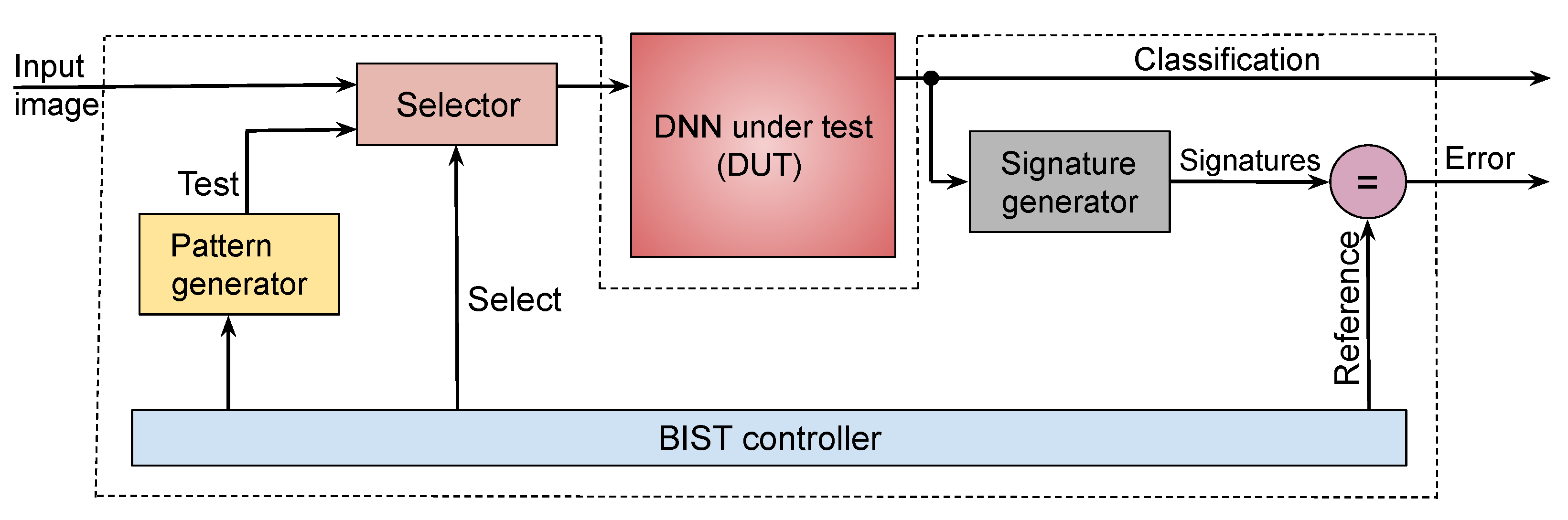
The proposed BIST infrastructure is shown in Figure 3. It operates as follows:

• The pattern generator contains logic to generate the pseudorandom test patterns, supplied to the hardware as 2D images. Three types of test patterns are generated: unstructured patterns in which pixel intensity values are chosen from either normal or uniform distributions; structured patterns that mimic edges and contours; and patterns from template images which capture chrominance information.
• The DUT is the quantized model obtained using the procedure described in Section 3. The ternary weights are mapped to the underlying crossbar architecture.
• Because the DUT is trained to classify the input into one of k labels, the response for each test consists of a one-hot-encoded predicted label wherein exactly one out of k output bits is set to 1. The signature generator compresses these bit patterns into a signature using cyclic redundancy checking (CRC) [27]. The signature generated per output line is compared to a previously calculated fault-free signature.
• The controller sequences and schedules tests. Control can be tied to a system reset so that the BIST occurs during system start-up or shutdown. The BIST can also be carried out when the system is idle, with the process being interruptible any time so that normal operation can resume.

5. Test-Pattern Generation

This section develops the TPG methods that generate pseudorandom and structured tests for the DUT.

5.1. Pseudorandom Testing

Test patterns are applied to the DUT in the form of 2D images where pixel-intensity values are chosen from a suitable distribution. In each case, we supply 10,000 test patterns to the DUT and calculate the ratio of covered faults to all possible faults.

Table 3. Fault coverage achieved by pseudorandom testing for various DNN models.

Workload	Model	Uniform Dist. (UD)	Normal Dist. (ND)
MNIST	ANN-3	34.02% (1416/4162)	92.04% (3831/4162)
	CNN-2	42.22% (1157/2740)	86.49% (2370/2740)
	LeNet-5	36.09% (1324/3668)	77.99% (2861/3668)
	AlexNet	52.67% (4577/8689)	93.72% (8144/8689)
FMNIST	ANN-3	43.83% (1779/4058)	95.29% (3867/4058)
	CNN-2	58.90% (2157/3662)	83.01% (3040/3662)
	LeNet-5	63.03% (3182/5048)	77.85% (3930/5048)
	AlexNet	64.74% (5496/8489)	91.58% (7775/8489)
CIFAR10	AlexNet	37.78% (11,304/29,922)	59.63% (17,845/29,922)
	ResNet-18	45.99% (38,840/84,447)	52.59% (44,412/84,447)

lists the fault coverage achieved for our DNNs. The simplest approach constructs tests $T_{\mathrm{UD}}$ using pixel-intensity values from a uniform distribution (UD) between $[0,1]$. However, the fault coverage achieved is very low. Conversely, tests, $T_{\mathrm{ND}}$, constructed using a normal distribution (ND) with appropriately chosen mean and standard deviation achieve much higher coverage.

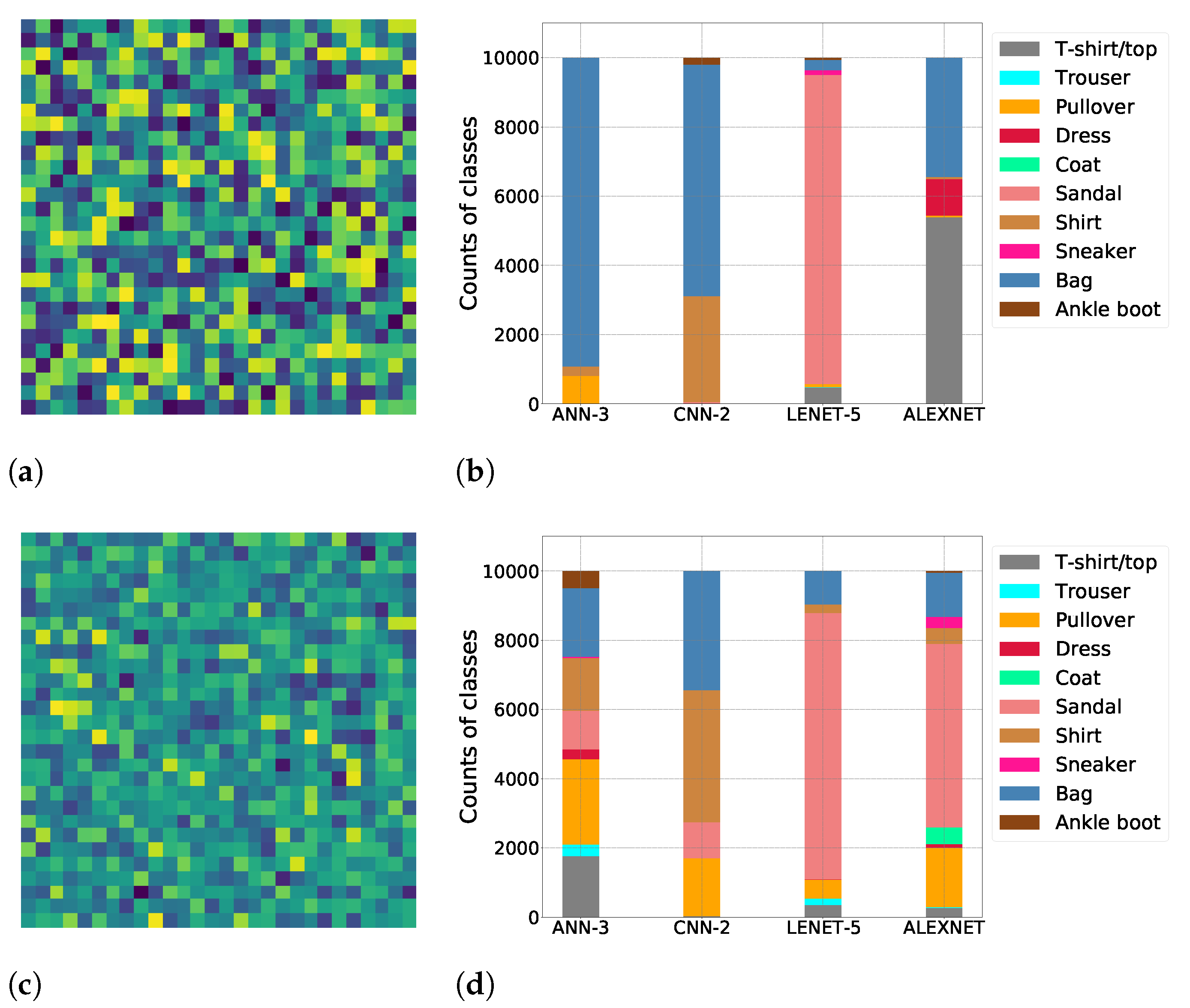
We use Figure 4 to gain insight into this phenomenon. The image in Figure 4a visualizes a sample test from $T_{\mathrm{UD}}$ and the stacked bar graph in Figure 4b shows the counts for the various output labels predicted by DNNs trained on FMNIST when supplied test patterns from $T_{\mathrm{UD}}$. Clearly, the models are unable to assign a diverse set of labels to these patterns. For example, ANN-3 assigns the “Bag” label to most of its tests. This behavior indicates the lack of diversity among the patterns within $T_{\mathrm{UD}}$—not enough weights are being sensitized because these patterns are not representative of the data used to train these models.

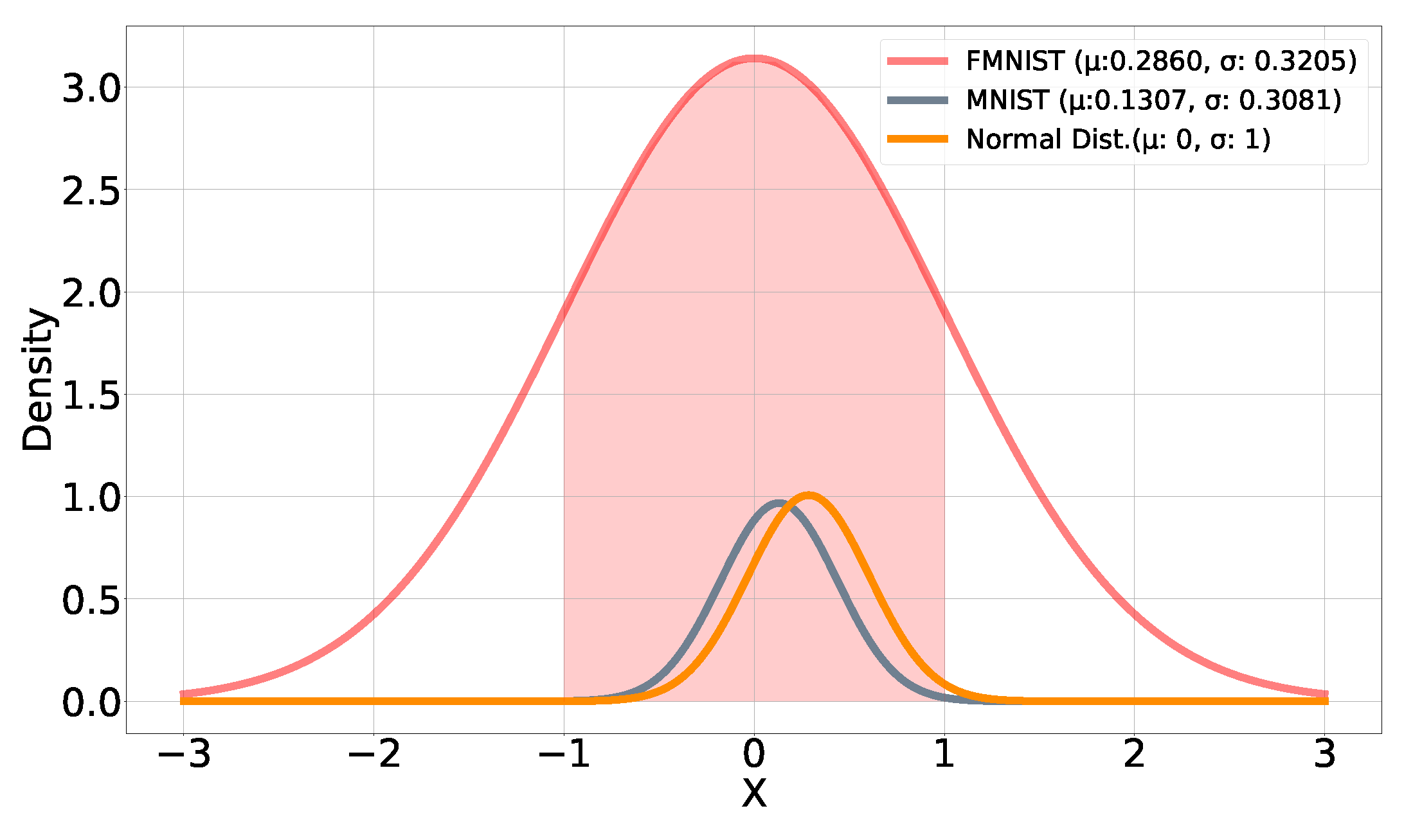
The rationale behind generating tests using an ND is best explained by describing how DNNs are trained. Instead of using raw feature values, these are standardized such that the transformed values are centered around the mean with standard deviation; if x is the raw value, then its scaled counterpart is obtained as $\tilde{x}=(x-\mu )/\sigma$, where $\mu$ and $\sigma$ denote the mean and standard deviation, respectively, of the training dataset. This is performed to improve the performance of the model and for a faster convergence of the optimizer as it learns the weights.

The summary statistics $(\mu ,\sigma )$ for the features within MNIST and FMNIST are calculated as $(0.13,0.31)$ and $(0.29,0.32)$, respectively. Once standardized, most pixel values for the MNIST and FMNIST datasets lie within one standard deviation of a normal distribution centered around a mean of zero, as shown in Figure 5, indicating that the DNNs were trained using data ranging mostly within $[-1,1]$. Therefore, pseudorandom tests are generated from a normal distribution having $(\mu ,\sigma )=(0,1)$ so that each test contains pixel-intensity values also mostly in the range $[-1,1]$. Figure 4c shows an example test image generated using values from this distribution. Because the DUT has been trained on similar values, these test patterns sensitize a greater fraction of the weights within it, resulting in an improved distribution in the count of predicted output labels (Figure 4d). If a weight becomes faulty, there is higher likelihood that the DUT will assign a label to one of the test images which is different from the one assigned in the fault-free case. This improves the fault coverage as confirmed by the results shown in Table 3.

Given its simplicity, we also generate tests using a UD whose values lie within the range of the raw pixel-intensity values found within the training dataset. The diversity is increased by applying different geometric transformations to each test, such as horizontal flipping, vertical flipping, random rotation, and affine transformation.

It is important to incorporate the summary statistics of the training dataset during the TPG to generate tests with a high likelihood of sensitizing faulty weights within the DUT.

5.2. Testing Using Structured Patterns

A CNN’s convolution layers extract features in the form of edges and contours for the subsequent fully connected neural layers. To improve upon the fault coverage in these DNN models, we generate structured patterns aimed at mimicking such features. The following primitive patterns are used as the basic building blocks.

• The $[0,f]$ primitive sets the intensity value of the current pixel to zero and that of its neighbor to f.
• The $[f,0]$ primitive sets the value of the current pixel to f and that of its neighbor to zero.
• The $[f,f]$ primitive sets values of both the current and neighbor pixels to f.

In the above, f denotes a value chosen from the normal distribution. To generate a structured pattern, m rows are chosen at random, and for each such row, we choose one of the three primitives, again at random, and replicate this primitive across the entire row. This process is repeated for n randomly chosen columns by replicating the chosen primitive along each column. The values at the intersection of a row and column are overwritten by the pattern used for that column, and the values outside of the shaded cells are set to zero. Figure 6 (top) illustrates this process. Once the basic structure is generated, we apply the same different geometric transformations used for UD-based tests to increase diversity. These simple operations result in complex test patterns such as those shown in Figure 6 (bottom).

5.3. Testing Using Template Images

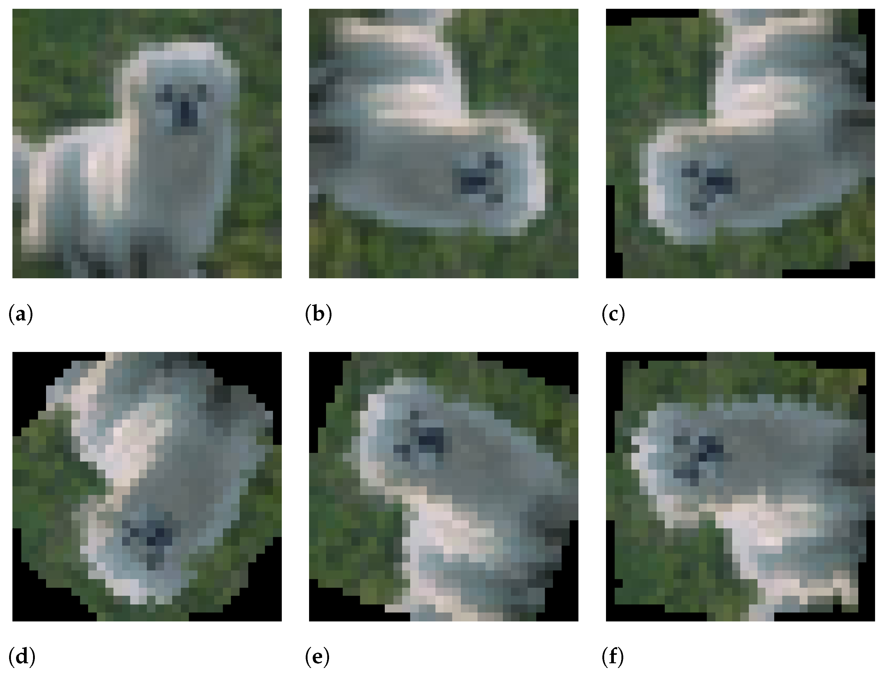
The above TPG method focuses on grayscale images. It generates edges, shapes, contours, and shadows but ignores the chrominance information present in the color images. These patterns may not achieve high fault coverage when applied to DUTs trained to classify color images. Thus, we develop the TPG method shown in Algorithm 1 which specifically targets color images which comprise red, green, and blue channels. We select, at random, template images from each class and generate test patterns by applying different geometric transformations on them to introduce diversity. This is similar to the approach used to capture statistical properties of the training dataset to create tests, but here, templates are used to capture the chrominance information present in the training images. Here, C denotes the number of classes, X is the set of training images, $x^{C_i}\subset X$ is the set of templates used per class, and $|x^{C_i}|$ is the number of templates per class.

Let $\{{\tau }_1,{\tau }_2,\dots ,{\tau }_k$} denote kgeometric transformations wherein each transformation ${\tau }_i$ applies a bijective function ${\tau }_i:template⟶I$. The transformations used for the TPG are: random rotation, horizontal flip, vertical flip, and affine transformation. Because a geometric transformation is any bijection of the set of template images to itself or to another such set with some salient geometrical underpinning, this one-to-one mapping between template images and the corresponding transformed images generates diverse test patterns which are all unique. Figure 7a shows a template image from CIFAR-10, and Figure 7b through Figure 7f show the corresponding test patterns generated using the TPG method discussed above.

Algorithm 1: TPG for color images using templates.

$TP\leftarrow \left\{\right\}$     /* Initialize test-pattern set */

for $j=1:C$ do

for $template$ in $x^{C_j}$ do

$angle\leftarrow random(0,360)$

$i\leftarrow random(1,k)$

$I\leftarrow {\tau }_i(template,angle)$

$TP\leftarrow TP\cup I$ /* Add new pattern to test set */

end for

end

5.4. Test Sequencing

We combine the different testing approaches discussed in this section to maximize the effectiveness of the BIST. Given a budget of N tests, the transition points for the test sequencing are determined as follows:

• Initialize the status of all faults to be uncovered.
• Generate N ND-based tests. Obtain the fault–coverage curve and find the point on this curve, say after $n_1$ tests have been applied, after which coverage levels off. Mark the faults detected up to this point as covered.
• Generate $N-n_1$ structured patterns and obtain the coverage for the remaining uncovered faults. Determine the point, after $n_2$ tests have been applied, at which coverage levels off and mark the detected faults as covered.
• Generate $N-n_1-n_2$ UD-based tests for the remaining uncovered faults. To reduce the test-set size, we can stop before exhausting the testing budget, when the coverage achieved by these tests stagnates.

To eliminate run-time overhead, transition points can be obtained via an offline analysis of the coverage curve.

6. Performance Analysis

We evaluate the efficacy of our TPG method in terms of the fault coverage achieved for the DUTs trained on grayscale and color images. We also evaluate the performance when multiple faults may be present in the system. The experiments reported here are performed using the PyTorch framework.

Note that when reporting fault coverage, we exclude dead neurons in the network from consideration. Though the ReLU activation function improves the DNN performance, there is a downside in that some ReLU neurons may “die” during training and always provide an output of zero for any input from the dataset. These neurons cannot discriminate between different inputs (and from a testing viewpoint, cannot be sensitized by any test pattern). In practice, dead neurons are detected and removed from the final network structure prior to mapping it on to the hardware.

6.1. Results for Grayscale Images

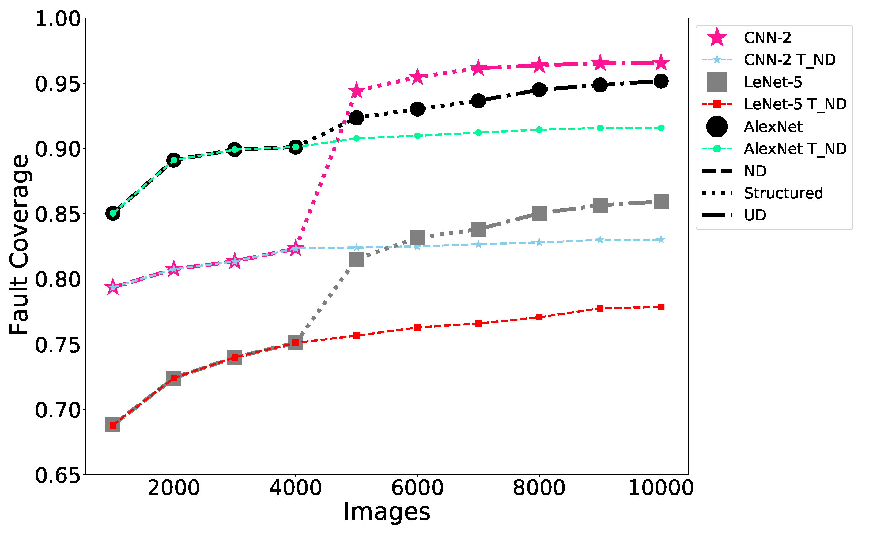
Assuming a budget of 10,000 tests, these are sequenced using the approach discussed previously: the first 4000 are chosen from $T_{\mathrm{ND}}$, the next 3000 are structured grayscale images, and the final 3000 tests are chosen from $T_{\mathrm{UD}}$. Figure 8 contains two curves for each of the three CNN architectures trained on FMNIST—one showing the fault coverage achieved via test sequencing and the baseline in which all 10,000 tests are chosen from $T_{\mathrm{ND}}$. By sequencing multiple types of tests, we are able to achieve higher coverage relative to the baseline case, especially for more complex CNN architectures such as AlexNet ( the results for MNIST are qualitatively similar and therefore are omitted from the paper). We theorize this is because tests $\in T_{\mathrm{ND}}$ sensitize easy-to-detect faults. Then, the structured tests along with tests $\in T_{\mathrm{UD}}$ which have been geometrically transformed further to increase their diversity sensitize the harder-to-detect faults, improving the fault coverage.

Table 4. Fault coverage achieved using 10,000 images from the training set versus our approach.

Workload	Model	Random (10 k)	Our Approach
MNIST	ANN-3	90.02%	98.94%
	CNN-2	96.27%	92.84%
	LeNet-5	94.62%	92.36%
	AlexNet	91.16%	96.78%
FMNIST	ANN-3	91.16%	96.78%
	CNN-2	98.77%	96.55%
	LeNet-5	96.94%	94.39%
	AlexNet	94.31%	95.18%
CIFAR10	AlexNet	91.54%	88.34%
	ResNet-18	90.46%	86.34%

compares the coverage achieved by our TPG method (column 4) against the case in which 10,000 random images from the MNIST and FMNIST training sets are used to detect faults (“Random” in column 3). This is not practical because these images must be stored onboard the device. Nevertheless, our approach achieves a comparable performance while incurring a negligible storage cost. For certain models and workloads, it outperforms “Random”, and in other cases, the coverage is within 3% of that achieved by “Random”.

6.2. Results for Color Images

Figure 9 shows the progression of the fault coverage as the tests are supplied to AlexNet and ResNet-18 trained on color images from CIFAR-10. The tests generated from the templates achieve better fault coverage for these images compared to the sequencing method used previously. The coverage is also compared against the case in which 10,000 random images are chosen from the CIFAR-10 training set (Table 4). Our TPG approach which uses two template images per class (twenty images in total) to generate the tests is comparable in performance while incurring a fraction of the storage cost. The coverage is within 5% of that achieved by “Random”.

6.3. Fault Coverage in the Presence of Multiple Faults

Recall that our TPG strategy assumes, at most, one fault present in the system. However, the tests derived under this assumption are usually applicable for multiple faults, because in most cases, a multiple fault can be detected by tests designed for the individual single faults that compose the multiple one. We now evaluate the fault coverage in the presence of two and three faults in the system. Given the combinatorial nature of this problem, the results are obtained by sampling potential double and triple fault sites.

Table 5. Fault coverage in the presence of double faults.

Workload	Model	$\uparrow \uparrow$ Transitions	$\downarrow \downarrow$ Transitions	Mixed Transitions
MNIST	ANN-3	96.23%	99.01%	98.53%
	CNN-2	94.78%	95.82%	95.47%
	LeNet-5	91.52%	95.95%	94.90%
	AlexNet	97.85%	98.71%	99.75%
FMNIST	ANN-3	96.21%	98.27%	99.74%
	CNN-2	95.46%	99.09%	96.94%
	LeNet-5	93.48%	95.62%	97.03%
	AlexNet	97.03%	97.12%	98.30%
CIFAR10	AlexNet	93.48%	96.88%	97.03%
	ResNet-18	90.04%	86.76%	97.66%

and

Table 6. Fault coverage in the presence of triple faults.

Workload	Model	$\uparrow \uparrow \uparrow$ Transitions	$\downarrow \downarrow \downarrow$ Transitions	Mixed Transitions
MNIST	ANN-3	97.90%	100.00%	97.66%
	CNN-2	97.08%	98.01%	94.45%
	LeNet-5	94.43%	97.80%	94.05%
	AlexNet	98.24%	8.93%	99.06%
FMNIST	ANN-3	96.94%	98.27%	99.36%
	CNN-2	96.55%	99.09%	96.57%
	LeNet-5	95.77%	97.93%	95.02%
	AlexNet	97.62%	97.46%	98.16%
CIFAR10	AlexNet	95.16%	98.05%	96.24%
	ResNet-18	91.15%	87.50%	98.27%

show the coverage achieved when two and three faults are present in the system, respectively. Let w denote a weight involved in the faulty transition. We consider the three cases shown in columns three through five in both tables.

• Transitions to larger synaptic weights ($\uparrow \uparrow$/$\uparrow \uparrow \uparrow$). Each potential fault site is set to a higher synaptic weight value than the original value. That is, $-w\to 0$ or $-w\to +W$.
• Transitions to smaller synaptic weights ($\downarrow \downarrow$/$\downarrow \downarrow \downarrow$). Each potential fault site is set to a lower synaptic weight value than the original value. That is, $+w\to 0$ or $+w\to -W$.
• Mixed Transitions. For double faults, one of the potential fault sites is set to a higher synaptic weight value, whereas the other is set to a lower value. That is, $-w_a\to \{0,+W\}$ and $+w_b\to \{0,-W\}$, where $w_a$ and $w_b$ are the fault sites involved. For triple faults, we consider all eight combinations involving weights $w_a$, $w_b$, and $w_c$, where $w_c$ is the third site.

Let us understand the results shown in Table 5 and Table 6. During image classification, the trained DNN assigns the highest probability to one of the neurons within the output layer to decide the class for the input image. More precisely, a dot product is performed between inputs from the penultimate layer and weights leading to the output neurons and is then passed through a sigmoid or softmax function to assign probabilities to output neurons. Suppose double and triple faults affect multiple weights of the output neurons. Consider the following cases:

• Transitions to larger synaptic weights ($\uparrow \uparrow$/$\uparrow \uparrow \uparrow$). For a test pattern, assume that inputs from the penultimate layer are $\{x_1,x_2,x_3,x_4,x_5,x_6\}=\{0.08,0.15,0.10,0.12,0.07,0.30\}$ and the trained weights leading to an output neuron are $\{w_1,w_2,w_3,w_4,w_5,w_6\}=\{1,-1,-1,1,-1,-1\}$. The dot product $\mathbf{x}.{\mathbf{w}}^T=-0.42$, which when passed through a sigmoid function $1/(1+e^{-{\mathbf{w}}^T.\mathbf{x}})$ results in a probabilistic value of $p<0.5$. Suppose a double fault results in both $w_3$ and $w_5$ transitioning to 1. The dot product will be $-0.08$, also leading to $p<0.5$. Hence, the test will not be misclassified. Now, consider a triple fault which causes $w_3,w_5,\mathrm{and}{w}_6$ to transition to 1. The dot product is $0.52$, resulting in $p>0.5$. This leads to a misclassification and, therefore, detection.
• Transitions to smaller synaptic weights ($\downarrow \downarrow$/$\downarrow \downarrow \downarrow$). For a test pattern, assume that inputs from the penultimate layer are $\{x_1,x_2,x_3,x_4,x_5,x_6\}=\{0.30,0.10,0.25,0.10,0.21,0.10\}$ and the trained weights leading to an output neuron are $\{w_1,w_2,w_3,w_4,w_5,w_6\}=\{1,1,-1,-1,1,1\}$. The dot product is $0.36$, leading to $p>0.5$. Suppose a double fault affects $w_2\mathrm{and}{w}_6$, flipping them both to 0. The dot product is $0.16$, leading to $p>0.5$. The test will not be misclassified. However, if a triple fault flips $w_2,w_5,\mathrm{and}{w}_6$ to 0, the dot product is $-0.05$ and $p<0.5$. This leads to the test being misclassified.

The above-described phenomenon is the likely reason that coverage in the presence of multiple faults is higher for most DNNs when compared to a single fault, and that triple faults are detected at a higher rate than double faults.

Consider coverage in the case of mixed transitions, which can involve the possibility of fault masking. Assume inputs $\{x_1,x_2,x_3,x_4,x_5,x_6\}=\{0.30,0.20,0.22,0.35,0.25,0.13\}$ from the penultimate layer and weights of the output neuron $\{w_1,w_2,w_3,w_4,w_5,w_6\}=\{1,-1,1,-1,1,-1\}$. The dot product is $0.09$, resulting in $p>0.5$. If a double fault causes $w_1\to -1$ and $w_6\to 1$, the resulting dot product will be $-0.25$ with $p<0.5$. Therefore, the test will be misclassified. However, if a triple fault results in $w_1\to -1$, $w_2\to 1$, and $w_6\to 1$, the dot product will be $0.15$ and $p>0.5$. The test will be classified correctly. Referring to column five in Table 5 and Table 6, this masking effect is the likely reason why double faults are detected at a higher rate than triple faults.

To summarize, our experiments indicate that tests generated to detect single faults can also perform effectively in the presence of two or three faults affecting the system.

7. Error Detection via Signature Analysis

Because the DNN is trained to classify the input into one of k labels, the response for each test consists of a one-hot-encoded predicted label wherein exactly one out of k output bits is set to 1. These bit patterns can be compressed using a well-known design based on cyclic redundancy checking (CRC) [27]. We associate a separate response compactor with each output line of the DUT and responses observed on the ith line (which could be 0 or 1) are compressed into a 16-bit signature using the characteristic polynomial $1+x^4+x^7+x^9+x^{16}$ (this polynomial is used in the Hewlett-Packard 5004A signature analyzer and also in many other applications requiring CRC). The signature generated per each output line is compared to a corresponding fault-free signature that has been previously calculated. When using a 16-bit signature, the probability that an incorrect response will go undetected is very low ($2^{-16}$).

8. Processing and Storage Overhead

Generating pseudorandom and structured patterns incurs minimal storage overhead because the tests are produced on demand. The overhead involves storing the summary statistics needed for the TPG along with the fault-free signatures. If templates are used for the TPG, a subset of the training images must be stored, and test patterns are generated on demand by applying the previously discussed geometric transforms to these images. The diversity and uniqueness of the generated tests means that the number of template images can be kept very small. For example, considering AlexNet and ResNet18 trained on CIFAR-10, we achieve a fault coverage of 88% by using just two images per class, which is twenty images in total.

The processing overhead incurred by our TPG method is modest. We report the test generation times on an Intel Xeon CPU operating at 2.20 GHz with 12 GB of onboard RAM. The time taken to generate a single pattern derived from the normal distribution $T_{\mathrm{ND}}$ is 0.1 ms and from the uniform distribution $T_{\mathrm{UD}}$ after geometric transformations is 1.6 ms. It takes 0.9 ms to generate a structured pattern, whereas generating a test from a template image by applying a geometric transformation incurs about 5 ms on average.

Because the BIST is non-concurrent, the host processor can perform the TPG when the application is idle. The BIST is interruptible at any time so that normal operation can resume. The TPG can be fully implemented using software modules, requiring no specialized hardware support.

9. Related Work

There is a large body of work on fault-tolerant systems, starting with early work on tolerating permanent faults in memory systems using error correcting codes [28], using redundancy to tolerate faults affecting logic circuits [29,30,31,32] and the routing fabric [33,34]. However, these approaches are not directly applicable to the crossbar-based architecture considered in this work.

There has been significant interest in using crossbar arrays to build accelerators for DNNs due to efficient in-memory computing and the parallelism that these arrays offer [1,2,3,4,35]. Researchers have developed various techniques to tolerate failures affecting crossbars. For example, Liu et al. developed methods to mitigate the effect of cell failures within crossbar arrays on the accuracy of the underlying calculations [35]. Robust training of neural networks on memristor-based crossbar arrays by compensating for the impact of device variations on the accuracy of multiply–accumulate operations has been proposed [36]. Yeo et al. developed circuit-level techniques along with a training algorithm to reduce the effect of stuck-at-faults within a crossbar array on the performance of the neural network mapped on to it [37]. Re-training the neural network in situ, however, risks reducing the device’s lifetime by increasing the chances of write-endurance failures [38]. Therefore, the applicability of these methods is limited to small networks.

Our work differs from those discussed above because it is a testing scheme rather than a method for fault tolerance. The BIST scheme aims to uncover faults affecting NVM cells within the crossbar array. The subsequent reconfiguration of the system is beyond the scope of this work.

Another line of related work addresses the design of fault-tolerant, systolic-array based DNN accelerators for high-defect rate technologies [6,7,9,39]. However, the developed methods are specific to the underlying systolic-array designs and do not apply to crossbar architectures. Though targeted toward a systolic array, the work described by Kundu et al. [7] is closest in relation to ours. Their TPG approach identifies images to serve as test patterns using the Euclidean distance between images from the neural network’s testing set. The idea is to identify a set of images which look very similar from the perspective of Euclidean distance but belong to different classes. This way, when hardware faults occur, images within this set are more easily prone to misclassification. However, a limitation is that computing pairwise Euclidean distance between high-dimensional images does not provide meaningful similarity information [40], and so the generated test set has reduced fault coverage for larger networks and images.

The test patterns generated by the approach in Kundu et al. must be stored on the device, and so, the storage cost will increase for larger DNNs because more tests are typically required to achieve good fault coverage. Therefore, from the perspective of storage overhead, our approach has key advantages related to the deployment on edge devices when compared to methods which require test patterns to be stored. Our technique generates pseudorandom tests on demand, and though a very small number of templates are used to generate tests for DNNs trained to classify color images, this overhead is minimal. Another important difference lies in the thoroughness of the validation experiments. Kundu et al. apply their technique to two simple models, a four-layer ANN and a six-layer ANN, in which the six-layer ANN is trained on the MNIST dataset. We have shown the broad applicability of our BIST method using both simple models as well as larger models such as AlexNet and ResNet-18. The workload considered includes both grayscale and color images.

10. Conclusions

We have shown that pseudorandom tests generated using information specific to the DUT achieve good fault coverage under the assumed functional fault model and that augmenting these tests with structured patterns further improves coverage. Very high fault coverage—greater than 95% on average—is achieved for DNNs trained on grayscale images which constitute an important class in image processing. DNNs trained to classify color images are more complex. Nevertheless, our TPG method which uses a tiny subset of template images to capture the chrominance information in color images achieves a fault coverage of 87% for these networks. Our results demonstrate the viability of BIST schemes to test DNN accelerators deployed on edge devices for image classification tasks.

A limitation of functional testing is the difficulty in evaluating the effectiveness of the test sequences at the structural level. Future work will evaluate the fault coverage achieved by the generated functional tests, using detailed structural models of crossbar hardware.

Our current work can be extended in various directions: (1) We have considered DNNs trained using the ReLU activation function, whereas other common functions such as the hyperbolic tangent, leaky ReLU, and Gaussian Error Linear Unit (GELU) can also be explored. (2) The TPG method can be extended to generate additional structured test patterns which could potentially increase the fault coverage, for example, patterns in which the thickness of the edges and contours are varied. (3) We can target faults due to the resistance drift, a phenomenon which affects PCM cells where the programmed resistance does not remain constant but increases gradually over time. The resulting cumulative changes in synaptic weights reduces the accuracy of multiply–accumulate operations performed within the DNN. Hence, the early detection of this accuracy loss before the network starts misclassifying input data would be useful. This requires developing online concurrent testing strategies which can observe and analyze intermediate values flowing within the DUT.