Memory Forensics-Based Malware Detection Using Computer Vision and Machine Learning

Abstract

Malware has recently grown exponentially in recent years and poses a serious threat to individual users, corporations, banks, and government agencies. This can be seen from the growth of Advanced Persistent Threats (APTs) that make use of advance and sophisticated malware. With the wide availability of computer-automated tools such as constructors, email flooders, and spoofers. Thus, it is now easy for users who are not technically inclined to create variations in existing malware. Researchers have developed various defense techniques in response to these threats, such as static and dynamic malware analyses. These techniques are ineffective at detecting new malware in the main memory of the computer and otherwise require considerable effort and domain-specific expertise. Moreover, recent techniques of malware detection require a long time for training and occupy a large amount of memory due to their reliance on multiple factors. In this paper, we propose a computer vision-based technique for detecting malware that resides in the main computer memory in which our technique is faster or memory efficient. It works by taking portable executables in a virtual environment to extract memory dump files from the volatile memory and transform them into a particular image format. The computer vision-based contrast-limited adaptive histogram equalization and the wavelet transform are used to improve the contrast of neighboring pixel and to reduce the entropy. We then use the support vector machine, random forest, decision tree, and XGBOOST machine learning classifiers to train the model on the transformed images with dimensions of 112 × 112 and 56 × 56. The proposed technique was able to detect and classify malware with an accuracy rate of 97.01%. Its precision, recall, and F1-score were 97.36%, 95.65%, and 96.36%, respectively. Our finding shows that our technique in preparing dataset with more efficient features to be trained by the Machine Learning classifiers has resulted in significant performance in terms of accuracy, precision, recall, F1-score, speed and memory consumption. The performance has superseded most of the existing techniques in its unique approach.

1. Introduction

Malware refers to malicious software, script, or binary code that performs malicious activities on systems to compromise the confidentiality, integrity, and availability of data. When malicious software compromises sensitive information/data without the knowledge or consent of the owner, confidentiality is lost. Availability is compromised when the malware causes information to become unavailable. Server unavailability or network infrastructure failure may make the data unavailable to end-users. Integrity is compromised when information is altered. In some instances, malware not only steals information, but also modifies it by inserting malicious code and waiting for the optimal moment to attack. Malware developers are consistently improving their techniques and building new strategies to bypass security controls.

Malware poses one of the most significant security threats to computer systems, and its timely detection and removal are vital for protecting them. Many free and commercial tools are available to generate variants of malware [1]. There are two types of malware: metamorphic and polymorphic. With each iteration, metamorphic malware is rewritten to create a new unique version. The changes in code make it difficult for signature-based antivirus software to recognize the same malicious program in different iterations. Despite the permanent changes to code, metamorphic malware functions in the same way. The longer that a given malware stays on a computer, the greater the number of iterations that it produces, making it more difficult for antivirus programs to detect, quarantine, and disinfect it. Polymorphic viruses are sophisticated file infectors that can modify themselves to avoid detection while maintaining the same basic routines. Polymorphic viruses encrypt their codes and use different encryption keys for each infection to vary the physical makeup of their files. They use mutation engines to change their decryption routines each time they infect a machine. Traditional security solutions such as signature-based, may not be able to detect them because they do not use static code. Complex mutation engines that generate billions of decryption routines make them even more difficult to detect. Polymorphic viruses are typically spread via spam, infected websites, and other malware. Notable polymorphic viruses include URSNIF, VOBFUS, VIRLOCK, and UPolyX or BAGLE. Polymorphic viruses are more dangerous when combined with other malicious routines. Both metamorphic and polymorphic types of malware increase the cost of analysis and can easily bypass anti-malware tools, such as antivirus applications [2].

A recent report claimed that cybercrime is up by 600% due to the COVID-19 pandemic [3]. Considering the alarming increase in security threats, novel approaches to defending against these attacks are crucial. According to AV-TEST, 99.71 million instances of malware were discovered in 2012 and more than 1.2 billion in 2021 [4]. The same report claimed that the Windows Operating System is a more frequent target of attacks than macOS, Linux, and Android. Another report claimed that the total global cost of malware attacks increased from USD 500 billion in 2015 to USD 6 trillion in 2021 [5].

Malware analysis is the process of examining the behavior of malicious software. It aims to understand how the malware operates and to determine the best methods for detecting and removing it. This entails analyzing the suspect binary in a secure environment to ascertain its characteristics and functionality and to develop robust defenses for the network. The primary goal of malware analysis is to extract meaningful information from a malware sample. The aim is to ascertain the capability of the malware, identify it, and contain it. It can also be used to identify recognizable patterns to treat and prevent future infections. There are many approaches to analyze a file, such as static, dynamic, and memory-based analyses.

Static analysis is the examination of a binary file without execution. It is the simplest method that allows for the extraction of metadata associated with the suspect binary. While the static analysis may not reveal all the necessary information, it can occasionally reveal interesting data that can help determine where to focus in the subsequent analysis. This quick analytical technique can be used to identify known malware with a low false-positive rate (FPR) [6]. However, it is unsuitable for use on unknown malware because the recorded signature may not recognize them even if only minor changes have been made to the code. This renders it unproductive and inflexible.

Dynamic analysis can be used to overcome these issues. In such analysis, the malware is executed in isolation or in a virtual environment (sandbox) to analyze the logs of its runtime behaviors [7]. The rate of malware detection using dynamic analysis is higher than that of static analysis, hence it can be used to understand the malware design better.

The dynamic approach does not translate the binary file into the assembly as the static analysis does. However, the intruder can use many techniques to fool the disassembler tool or program [8]. The dynamic analysis uses system calls, memory modification, registry modification, and network information [9]. Its drawbacks include, but are not limited to, an inability to identify disguised processes and behavior, privilege escalation, and nested virtualization [8]. The common tools for dynamic analysis include IDA Pro, Lida, Peview, PeStudio, Process Explorer, TDIMon, RegMon, and Wireshark [10]. Recently developed techniques use a memory-based analysis of malware/benign files. This technique is also referred to as memory analysis or memory forensics. The aim is to understand the behavior of malicious files or programs in a computer’s volatile memory. It can be used, for instance, to identify suspicious hidden processes in memory, such as logic bombs [6]. In this approach, the entire volatile memory (RAM) of the victim computer system is dumped for analysis [9]. The log obtained through this approach contains runtime-specific information, such as a list of running processes, active users, open network connections, and registry information [11].

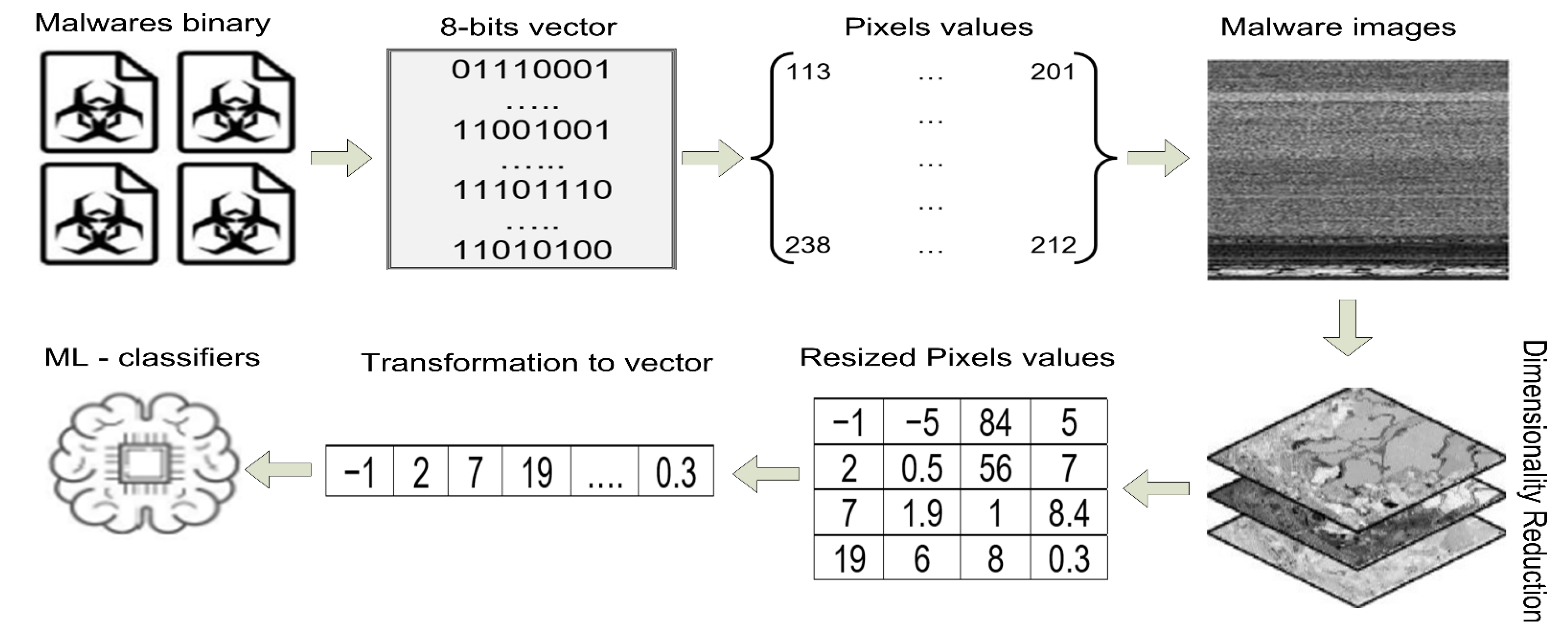
Many researchers have proposed a visualization analysis [12] of malware detection that negates the need for domain expertise to manually extract the artifacts [13]. In such an approach, malicious files are converted into images [14,15], and the dimensions of the resulting images vary based on the sizes of the malware files [16]. The literature review presents two types of image channels: a grayscale image [14,17,18] with a single channel and an RGB image [15,16] with three channels. Various dimensionality reduction and feature extraction techniques are used to reduce the size of malware images and to extract their pertinent characteristics. However, these techniques are either inefficient at extracting important features or computationally expensive, or memory intensive.

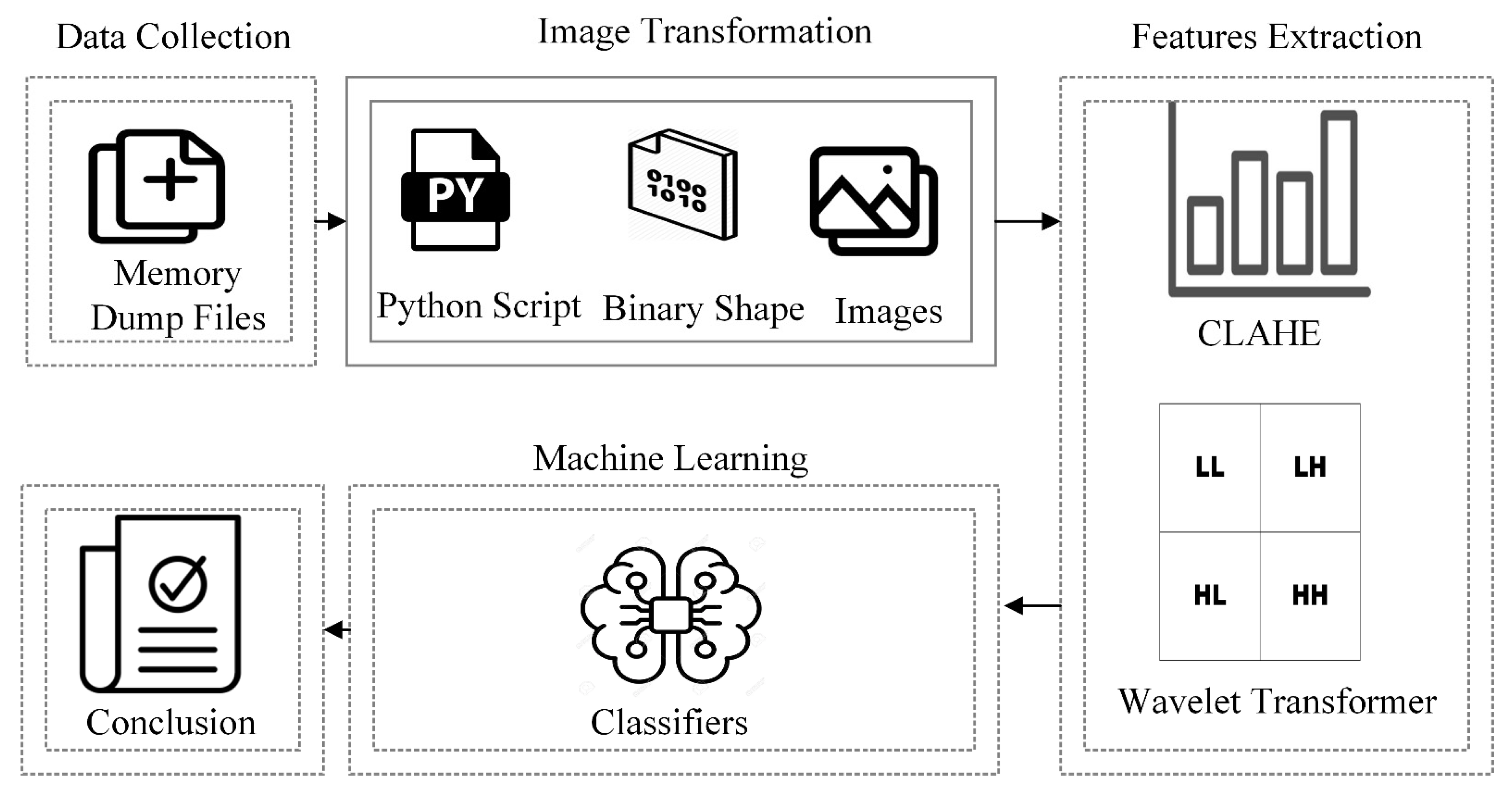
This paper presents a new technique for malware detection based on memory-based analysis and computer vision by using machine learning. The malware files are executed in a controlled virtual environment, and the data in memory are dumped into dmp files that are then converted into RGB images in PNG format. The Contrast Limited Adaptive Histogram Equalization (CLAHE) equalization technique is used to reduce noise and localize the contrast values of pixels in the images [19,20]. 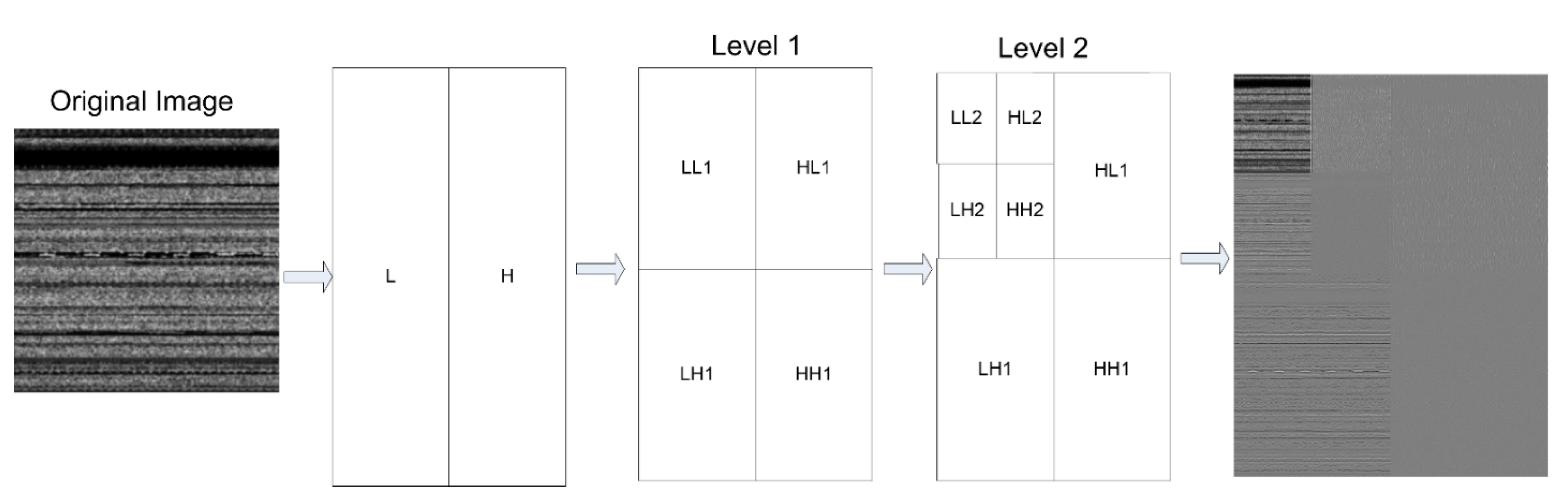The wavelet transform [21,22,23] is used to compress the images without losing the essential features for levels 1 and 2 that provide two versions of the dataset of images, consisting of images containing 112 pixels and 56 pixels. Finally, both versions of the dataset are fed into machine learning classifiers for training and testing. We compared our model with other machine learning algorithms to assess its performance.

The main contributions of this work are in two folds:

• A new technique that prepares malware datasets with efficient and significant features with the following novelty steps:

  ○

  An efficient technique that eliminates noise in images.

  ○

  A memory-efficient technique that reduces images size without compromising its sensitive information.

• Identification of the best machine learning classifiers that return the optimized and best performance based on the prepared datasets.

The remainder of this paper is organized as follows: Section 2 discusses related work in the area, Section 3 presents the methodology, Section 4 details its implementation and the results, and Section 5 provides the conclusions of this paper as well as directions for future research.

2. Background and Related Work

Machine learning and deep learning techniques have been used extensively to detect malware. Understanding the most critical features of malware files is essential for training any model to identify them. The patterns or behaviors of these malicious files need to be examined to gain information related to the intentions of the malware developer.

A signature is the characteristic footprint or pattern of a malicious attack on a computer network or system. This pattern can be a file or a byte sequence of network traffic. It can also be the unauthorized execution of software, network access, directory access, or the use of network privileges. Signature-based detection is a popular method for detecting software threats, including viruses, malware, worms, and trojans. Antivirus manufacturers use this method to create an appropriate signature of malware files and compare it with known suspicious files. 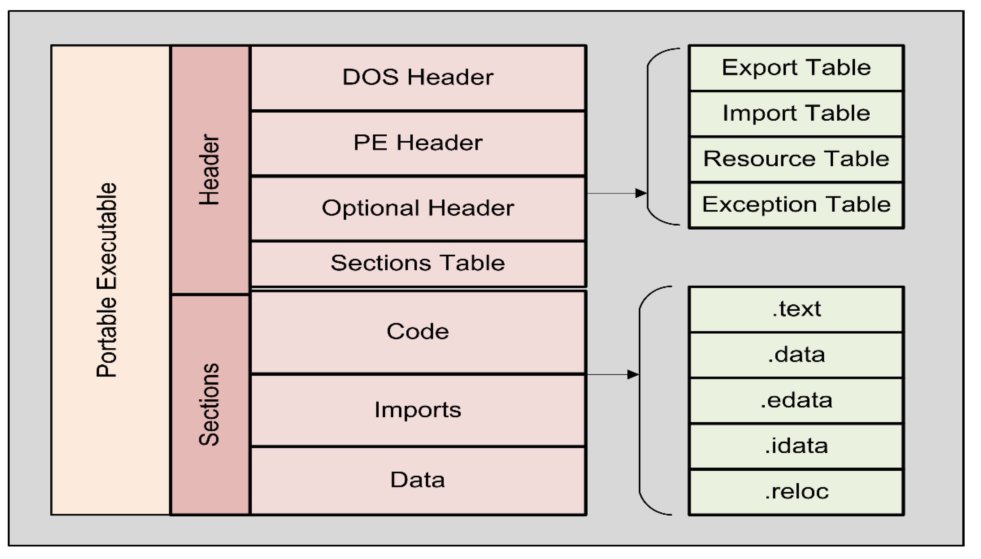This method is beneficial because it is quick and accurate [24]. Programs/tools such as PeStudio, Process Hacker, Process Monitor, ProcDt, and X64dbg are used for the static analysis of malicious files. It is important to understand the portable executable (PE) structure of the malicious file to effectively use these tools. The PE file format includes a Disk Operating System (DOS) header, DOS stub, PE file header, section tables, PE section, and transport layer security (TLS) section. Figure 1 shows the structure of the PE format used in 32-bit and 64-bit versions of Microsoft Windows.

The DOS header begins with 64 bytes for any PE file. This section reveals the extension of a particular file. An error message such as “This program cannot be run in DOS mode” appears on the screen when the DOS stub is used. Extra information, such as the size and location of the code can be found in the PE header. Other subsections include the Signature, NumberOfSections, SizeOfOptionHeader, SizeOfRawData, and PointerToRawData. The sections provide a logical and physical distinction between the various components and help load the executable file into memory during execution. They contain information on the Dynamic Link Library (DLL) and other metadata.

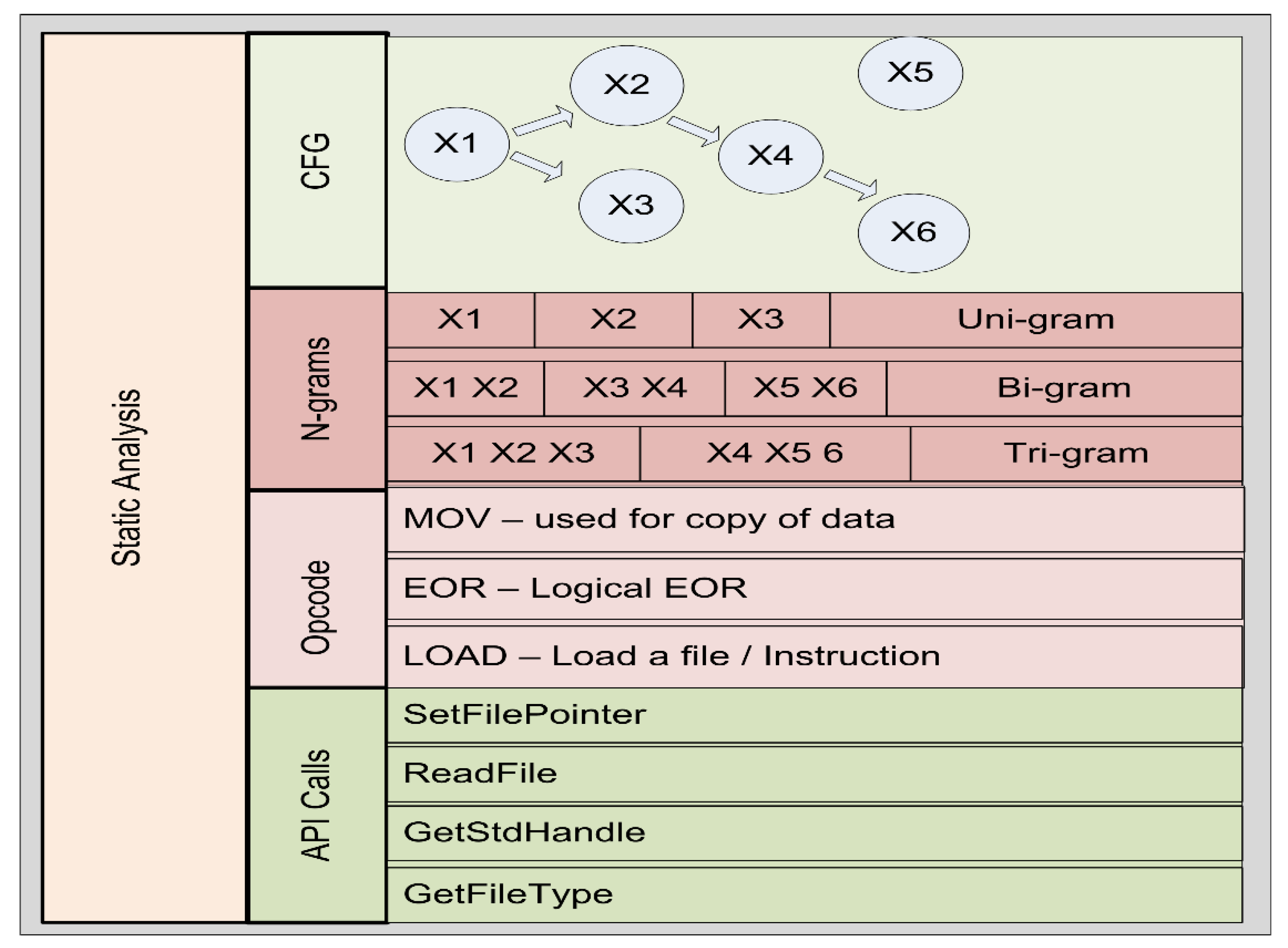
The structure of the PE file is analyzed to pull informative features from it. The static analysis uses a variety of approaches for analyzing and extracting such characteristics, including Application Programming Interface (API) calls, control flow graphs, n-grams, and operation code (opcode) [25]. Figure 2 shows the approaches to static analysis.

An API is software that enables two unrelated applications to communicate with each other. It functions as a bridge that accepts requests or messages from one application and delivers them to another by interpreting them and enforcing protocols in accordance with the given specifications. It links everything together and ensures that software systems operate in sync. APIs are often transparent to users and provide a plethora of options for software applications. They operate by allowing restricted access to a subset of the software’s functionality and data. This enables developers to access a particular program, piece of hardware, data, or application without requiring access to the complete system code.

Table 1. Windows-supported APIs.

Windows APIs	Description
CreateProcess	Create a new process
CreateMutex	Open an existing mutex
CreateThread	Create a new thread
CreateFiber	Create a new fibre
ExitProcess	Terminate the current process
WaitForSingleObject	Block on a single semaphore
LeaveCriticalSection	Release the lock on critical
SetPriorityClass	Set the priority class

presents a collection of commonly used Windows-based APIs and their descriptions.

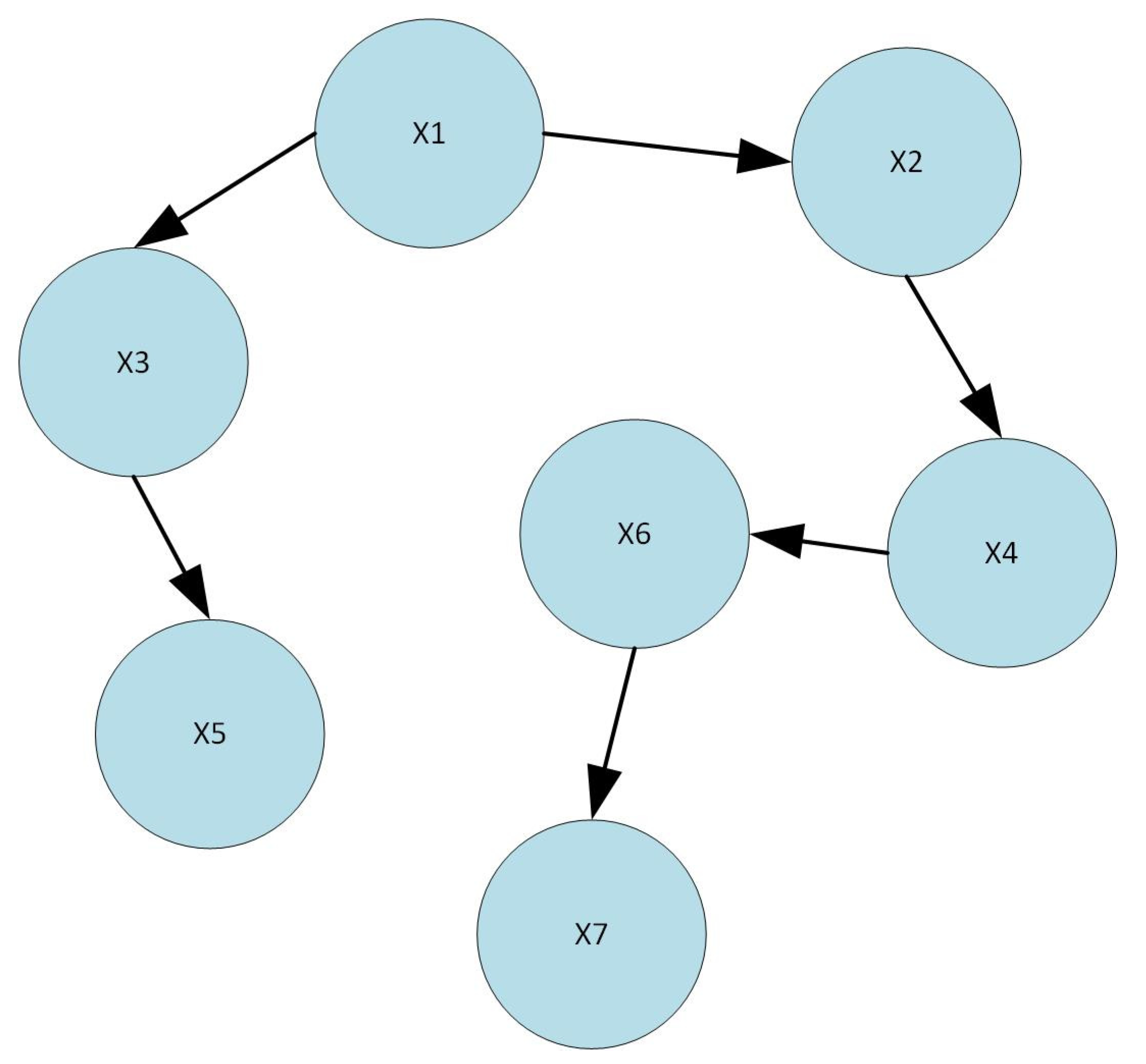
A control flow graph (CFG) is a graphical depiction of the several pathways that the code of a computer program may follow. A CFG is composed of a sequence of symbols called nodes that are linked by arrows that indicate the path taken by each node to reach the next one. Each node represents a single line or a group of lines of crucial computer code. Regardless of the mechanism used to generate a CFG, they are always read in the same way: A CFG resembles a flowchart. Creating it serves a variety of critical purposes, one of which is to determine if any portion of the computer program is useless. This can be determined by the control flow diagram and is a simple operation. Any node that is not connected to the rest of the nodes by an arrow is suitable for deletion. In addition, when program execution is restricted to a single node, a CFG can be used to help isolate problems, such as infinite loops. The condition that needs to be satisfied is to move to the node to which each arrow point is represented by an arrow on the diagram. As a consequence, situations in which this requirement is never satisfied can be recognized because the program cycles back to the previous node. A CFG may also be used for the development of a software dependency graph. This graph illustrates the interdependence of several components of a program and is used to ensure that the program code is run in the correct order. Figure 3 shows a general view of a program or application flow controlled by the CFG, where X1 through X7 are the names of the nodes, and it has values. These nodes are used in conjunction with conditional statements such as IF, IF-ELSE, WHILE, etc. Such a procedure always begins at X1 and advances until the condition is met. It is faster than other approaches to static analysis for analyzing file behavior [26].

X1–X7 represents nodes that are used in conjunction with conditional statements, such as IF, IF-ELSE, WHILE, etc. These conditional statements begin at X1 and advance until the condition is met.

The n-gram is another widely used approach to static analysis. An n-gram is a sequence of n consecutive elements in a text document. We can use words, numbers, symbols, and punctuation to create these items. Text classification, text generation, and sentiment analysis are all common uses of this method. When analyzing malware, the n-gram is used with an opcode, a string sequence, and a sequence of API calls. The n-gram keeps track of how many words exist in malware files. A variety of n-grams were used in the literature, e.g., unigram, bigram, trigram, four-gram, and five-gram.

The opcode-based approach to static analysis is a subset of a machine language instruction that specifies the operation to be performed. A program is defined more precisely as a sequence of organized assembly instructions. An instruction is a pair or list of operands consisting of an operational code and a list of operands. These operation codes, such as MOV, JUMP, PUSH, and POP, are often used to inspect a file and determine its behavior. In [27], a deep learning-based convolutional recurrent neural network was used in conjunction with the opcode sequence to detect malware. The researchers had to shorten the extended opcode into a sequence to extract the opcode from suspect PE files.

Dynamic analysis can be used to view the malicious file at multiple levels of detail. At a low level, we monitored the binary code, whereas changes to the registry or file system are examined at a high level [25]. In contrast to static analysis, which examines the binary code, patterns, and signatures of malicious files, dynamic analysis examines file behavior. Malware developers continually try to find new ways to evade detection or incorrectly classify their intent. At least 10 methods of attack are typically employed by malware developers in each sample [28], which is why malware analysts must be aware of these evasive techniques [29]. Feature extraction relies primarily on domain expertise and is conducted manually. The features are extracted by collecting all events, including API calls, network logs, and registry information. Various combinations of approaches, such as API + DLLs, API + summary information, DLL + Registry, Registry, DLLs, API calls, and Registry + summary information + DLLs + API, are used to enhance malware detection [30].

Approaches to malware analysis based on memory analysis have become popular in the last two years. This approach is efficient and precise at detecting and classifying malware. Two critical phases are involved in implementing a memory forensics-based analysis. Memory acquisition is the first, where researchers attempt to execute suspicious files in a simulated control environment and then dump the volatile memory by using a free or a commercial tool (Memoryze, FastDump, Dumpit) [31]. In the second phase, the dump file is analyzed by using Volatility and Rekall tools. The domain-specific characteristics are manually extracted.

Memory Analysis/Memory Forensics

In [17], the researchers illustrated how files from a computer’s memory dump could be used as a heuristic environment for malware detection. This approach examines the registry activity, imported libraries, and API function calls in three features of memory images. The researchers in [17] examined the performance of the technique for malware detection after evaluating the significance of each feature. The method achieved an accuracy of 96% by using a support vector machine-based model fitted to data on the registry activity.

In [32], the researchers demonstrated forensics by using memory dumps and static malware analysis. Malware that conceals its behavior or artifacts can be discovered by using this approach. Static analysis was used to decrypt and pack malware samples in order to identify hidden activity. The authors categorized 90% of the data as within the required limits and claimed that their approach could be used in a variety of strategies to increase the rate of detection.

In [33], researchers provide novel solutions to problems, such as user-mode/kernel-mode rootkits, calling undocumented functions, calling native functions that are not hooked, and custom WinAPI function implementation. The authors contributed to the trigger-based memory analysis approach, which automatically used exciting events to take memory dumps in the system. Security researchers can thus obtain comprehensive information on executables. Combined with other techniques of memory analysis, this method can improve security and provide helpful information on malware.

Similarly, the researchers in [34] proposed a trustworthy and safe architecture for detecting malware on virtual machines in the private cloud of an organization. The authors obtained safe and trustworthy volatile memory dumps from a virtual machine (VM) and used the minhash technique to examine the data in them. This approach was assessed in a series of increasingly demanding tests that also tested the efficacy of several classifiers (similarity-based and machine learning based) on real-world malware and legitimate apps. The authors claimed that the proposed framework could identify known, new, and unknown malware with an extremely high TPR (100% for ransomware and RATs) and very low FPR (1.8% percent for ransomware and 0% for RATs).

In [35], the researchers introduced a sandbox design by using memory forensics-based techniques to provide an agentless sandbox solution independent of the VM hypervisor. It leveraged the introspection method of the VM to monitor malware running memory-related data outside the VM and analyzed its system behaviors, such as the process, file, registry, and network activities. The authors evaluated the feasibility of this method by using 20 advanced and eight script-based malware samples. They demonstrated how to analyze malware behavior in memory and verified the results by using three types of sandboxes. The results showed that this approach could be used to analyze suspicious malware activities, which is helpful for cyber security.

In [36], the researchers presented a sample malware memory dump-based technique developed by using an API trigger-based memory dump. They updated the Cuckoo sandbox to implement it. The API trigger was replaced with a hooking approach in Cuckoo. This means that API calls and memory dumps were always synchronized. The authors claimed that because the encrypted IP address was stored in memory, it was possible to retrieve the plain text and identify hidden information before it was hidden again by the malware.

In [37], the researchers provided a strategy to detect malware that uses forensics-based techniques to recover malicious artifacts from memory and combines them with data obtained during malware execution in real time. They also applied feature engineering techniques before training and testing the dataset on machine learning models. Following the implementation of the SVM, the results showed a significant improvement in terms of accuracy (98.5%) and the false-positive rate (1.7%). The authors claimed that the limitations of dynamic analysis could be circumvented by including important memory artifacts that reveal the true intent underlying malicious files.

In [6], the researchers demonstrated a memory forensics-based approach for extracting memory-based features to facilitate the detection and classification of malware. The authors claimed that the extracted features could be used to reveal the behavior of the malware, including the DLL and process injection, communication with command and control, and gaining privileges to perform specified tasks. They used feature engineering to transform the features into binary vectors before training and testing the classifiers. The experimental results showed that this approach could achieve a classification accuracy of 98.5% and a false positive rate of 1.24% when the SVM classifier was used. The authors also constructed a memory-based dataset with 2502 malware files and 966 benign samples and made this publicly available for future research.

In [38], the researchers proposed three strategies to prevent the memory space of malevolent users from being exposed to tools of analysis. Two of these tactics, page table entries and structures that handle the user’s memory, also require elevated privileges. The third makes use of shared memory but does not completely create and test all approaches to the Windows and Linux operating systems to demonstrate the viability of the strategy. The authors provided two Rekall plugins to automate the finding of shared memory.

In [30], the researchers provided a technique for memory imaging and pattern extraction from suspicious data. The authors claimed that malware samples from the same families have comparable 3D patterns of memory access defined by the sequence of access relative to the sequence of computing instructions, the instruction address, and the memory location accessed. This technique was tested on datasets of malicious and benign software. The results showed that comparable malware samples could be recognized by using memory images.

In [9], the researchers proposed criteria for signature matching and string pattern matching for the YARA scanner to detect malicious programs in RAM dumps. In order to save time, a GUI-based automated forensics toolkit was used instead of the command-line technique of the volatile memory forensic toolkit for analyzing processes. The RAM image is inspected using a built-in program to detect and remove possibly dangerous apps. According to the study, malware forensics can be applied to the recorded processes to delve into the origins of the attack and determine the specific cause.

In [31], the researchers combined the VMI, memory forensics analysis (MFA), and machine learning at the hypervisor to form an enhanced VMM-based guest-assisted A-IntExt introspection system. They used the VMI to inspect digital artifacts from a live guest OS to obtain a semantic perspective on the processes. The proposed A-IntExt system includes an intelligent cross-view analyzer (ICVA) that scans VMI data to discover hidden, dead, and suspicious processes while anticipating indications of early malware execution on the guest OS. Machine learning algorithms were used to identify malicious executables in the MFA-based executables. The A-IntExt system was tested by running a large number of malware and benign executables on the live guest OS. It obtained an accuracy of 99.55% and an FPR of 0.004% when detecting unknown malware on a generated dataset. The A-IntExt system exceeded real-world malware detection at the VMM by over 6.3%.

Similarly, in [16], the researchers proposed a technique for detecting malware that involves collecting the memory dumps of suspicious programs and converting them to an RGB image. First, the authors described the proposed approach. Unlike past research, they sought to gather and exploit memory-related data to form visual patterns that can be identified by using computer vision and machine learning algorithms in a multi-class open-set recognition regime. Second, they used a state-of-the-art manifold learning approach called UMAP to improve the accuracy of malware identification by using binary classification. They tested the method on a dataset of 4294 samples containing ten malware families and benign executables. Finally, GIST and HOG (histogram of gradients) descriptors were used to create their signatures (feature vectors). The collected signatures were categorized by using j48, the RBF kernel-based SMO, random forest, XGBoost, and linear SVM. The method yielded an accuracy of 96.39% by using the SMO algorithm on feature vectors based on GIST + HOG. The authors also used a UMAP-based manifold learning technique to increase the accuracy of detection of unknown malware by average values of 12.93%, 21.83%, and 20.78% for the random forest, linear SVM, and XGBoost algorithms, respectively.

3. The Methodology

Our proposed technique consists of four basic steps for malware detection and classification, namely, (i) data collection, (ii) image transformation, (iii) feature extraction, and (iv) training and testing using machine learning classifiers. The data collection phase provides information on the dataset, such as the number of classes and files and the file type. Image transformation involves converting the data in the memory dump of the malware into images. Feature extraction involves obtaining essential features from the images. We use two approaches in this step: CLAHE and the wavelet transform. The CLAHE approach helps eliminate noise while the wavelet transform reduces the number of dimensions of the images. The last step in our proposed technique involves training and testing the data by using machine learning classifiers. The whole methodology in our proposed technique is shown in Figure 4.

3.1. Data Collection

The data can be in any format, including video, audio, images, and electronic impulses. They must be gathered from a trustworthy source and need to be pre-processed. A limited number of datasets, such as the Microsoft Malware Classification Challenge, Malicia, Malimg, and Malevis, are available to this end. The BIG2015 (Microsoft Malware Classification Challenge) dataset contains 200 GB for training and 200 GB for testing. It contains nine malware classes in 10,859 files [39]. The Malicia dataset contains eight classes of malware containing 11,363 samples [40], and the Malimg dataset is used for multi-class classification. It contains 25 malware families over 9339 images. The number of files belonging to each family varies, which makes it a highly unbalanced dataset [14]. The Malevis dataset contains 26 classes, of which 25 are malware, and one is benign. The dataset contains RGB images. It contained 9100 training images and 5126 validation images. We used another dataset provided in [16] that contains memory dump files executed in a virtual control environment. It consisted of 4294 portable executables classified into 11 categories (10 malware + one benign class), as shows in

Table 2. Memory dump dataset consisting of ten classes of malicious software and one class of benign software.

Category	Classes	Quantity
Adware	Adposhel	457
Worm	Allaple.A	437
Adware	Amonetize	436
Worm	AutoRun-PU	196
Adware	BrowseFox	190
Trojan	Dinwod!rfn	127
Adware	InstallCore.C	467
Adware	MultiPlug	488
Trojan	Vilsel	389
Virus	VBA	499

.

Generally, adware is used to display or download advertisements as banners or pop-ups when a user goes online in order to generate revenue for the developers. Worm is a self-replicating program that attempts to spread to other computer networks in order to infect them. Trojans are malicious programs that look legitimate but take over your computer. Trojans severely affect, steal, or otherwise harm your data or network, whereas computer viruses are malicious code that spread from device to device. These self-copying threats are a subset of malware designed to damage or steal data.

3.2. Image Transformation

Extracting critical characteristics from a file requires a significant amount of effort and domain-specific expertise. The absence of any critical characteristic might degrade the performance of a machine learning model. One of the contributions of this study is to convert malicious dump files into images so that their characteristics can be extracted automatically. This visualization technique bridges the gap between computer vision and sequences of executable bytes. To convert binary files (DMP) files into images, we used the Python tool binary2image. The script converts a DMP file into binary and then into RGB (.png) format. The RGB image has three channels—R (Red), G (Green), and B (Blue)—that consume a large amount of memory and increase the cost of computation. The objective of converting images into the png format is to avoid loss of data [12]. This technique for compressing files works on both image and audio files. All the images are converted into grayscale, and images with a diversity of dimensions, ranging from 1024 pixels to 1580 pixels, are obtained. Scaling the image to a square size reduces its visual information, but the loss is not significant [16]. Classification, clustering, and other machine learning techniques require feature vectors of equal length. A computer vision-based technique thus must generate feature vectors of equal size (i.e., signatures) to represent images. In this work, all images are resized to dimensions of 224 × 224. Figure 5 illustrates the images of malicious and benign files after conversion.

Table 3. Pseudocode of an algorithm used for the transformation of dump (binary) files into images.

Algorithm 1: Transformation algorithm for dump (binary) files to RGB images
	Input: A path to a dataset of memory dump files
	Output: Transformation of RGB images with various dimensionality
	Start Set B a list of memory dump files Set weight 1024 Set data an empty list [ ] For bi in length(B) where bi integer numbers range from 0 to n.   height = calculate_size_byte(Bbi)   size = weight × height   image = Bbi.dimension(size), where Bbi indicate the dump (binary) files range from 0 to n.   image.save[‘PNG’]   data.append[image] End For End

illustrates the pseudocode of the algorithms utilized by the proposed techniques. Algorithm 1 describes how to convert dump files (binary) into color images as ‘PNG’ format.

3.3. Feature Extraction

Feature extraction is a dimension reduction technique that reduces a large set of raw data into more manageable groups for processing. These large datasets contain variables and require significant computation power to process them. Feature extraction is the term used to describe methods for selecting and combining variables into features to reduce the amount of data that needs to be processed while exclusively and accurately describing the original information.

3.3.1. Contrast-Limited Adaptive Histogram Equalization (CLAHE)

Global histogram equalization (GHE) is a widely used technique for increasing the contrast of images by extending their range of intensity. The equalization of histograms entails mapping one distribution to another so that the provided histogram is transformed into a more uniform and broader range of intensity values. It is accomplished by using the cumulative distribution function to normalize the distribution of intensity to yield a uniform distribution. Despite its impressive performance, histogram equalization can alter the original brightness of the input image, add irritating artifacts, and increase the noise in it. CLAHE can overcome the limitations of GHE. It is used to increase the complexity of a grayscale image by operating on discrete parts of it, referred to as tiles, instead of the entire image. The difference between tiles is increased such that the histogram of the output of a given tile matches the histogram set by using the appropriate parameter. Adjacent tiles are then connected by using bilinear addition to eliminate any artificially imposed constraints. Complexity, especially in homogenous regions, can be limited to avoid enhancing any noise in the image. CLAHE conducts histogram equalization in tiny patches with great precision and contrast limitation.

In the proposed technique, we used a computer vision function of CLAHE with the “cliplimit” set to 0.02 and “tileGridSize” set to (4,4). Figure 6a,b show the differences in images before and after the implementation of CLAHE.

The difference between the histogram equalization of the image before and after the use of CLAHE is shown in Figure 7a,b. CLAHE changes the pixel values of the image from high to low. It is an extension of Adaptive Histogram Equalization (AHE) that modifies the computation of enhancement by imposing a user-specified level on the height of the local histogram. Thus, augmentation is minimized in extremely uniform portions of the image to prevent enhancing noise and reduce the impact of edge shadowing. High-intensity values (black color) are converted into lower-intensity values (grey).

3.3.2. Wavelet Transform (WT)

The wavelet transform is derived from the Fourier transform and alters the representation of a function or signal (waveform). The Fourier transform is applied to time-based patterns. It computes each cycle to provide the amplitude, rotation, and offset. It is used in signal processing. In the context of image processing, it splits the given image into sine and cosine components. The output image is in the frequency domain or the Fourier domain, while the input image is in the spatial domain. This technique applies to a wide variety of tasks, including image filtering, reconstruction, compression, and analysis. The primary disadvantage of the Fourier transform is that it creates a signal with only a frequency domain and does not allow for spatial localization. The wavelet transform overcomes these constraints. It is a finite-length oscillation function that combines images and audio with localized vibrations. A review of the literature shows that it is used in a variety of applications, including signal processing, image reconstruction, and noise reduction. It is used to compress an image without sacrificing its resolution. Wavelet transforms are grouped into three categories: continuous wavelet transform, discrete wavelet transform, and wavelet transform with multi-resolution (MR) capabilities. Continuous wavelet transform is often used in time-frequency analysis to filter the time-localized frequency.

By contrast, the discrete wavelet transform compresses the signal/image, whereas the multi-resolution transform helps analyze the signal at multiple frequencies and resolutions. It provides excellent temporal resolution at a low frequency. Noise can be removed by using the wavelet transform through a Gaussian technique to compress the image. It separates the input signal into several scales, each representing a different space–frequency component of the original signalization. In the proposed technique, the CLAHE images are downscaled by using the wavelet transform. Depending on the level of implementation, it divides the images in half. In this context, we image with dimensions of 224 × 224 pixels that are downscaled to 112 × 112 pixels by using the wavelet transform at level 1. Similarly, level 2 contained images with dimensions of 56 × 56 pixels. We constructed two datasets of memory-related images with dimensions of 112 × 112 and 56 × 56. We determined whether the combination of CLAHE and the wavelet transform is suitable for reducing noise, memory, and the cost of processing via dimension reduction.

We used the pywt library, a Python package for wavelet transforms. It contains various families, including Haar, Daubechies, and Symlets. We considered the Daubechies (db) family here. The signal extension mode is used to present digital signals on the computer. Because it is a finite array of values, some extrapolation of the input data is required prior to performing the discrete wavelet transform by using cascading filter banks. We used the periodization mode. To compress the images, we considered two levels of the wavelet transform. Figure 8 depicts a general view of the wavelet transform for levels 1 and 2.

Table 4. Pseudocode of the algorithm used to denoise and compress the malware’s images.

Algorithm 2: The algorithm to convert images to list.
	Input: Path to the malware’s images
	Output: Transform into lists (dataset, labels)
	Start Set path to data Set X empty list [ ] Set Y empty list [ ] For i in length(path)   X.append[datai]   Label = Xi.label   Y.append[Label] End For End
Algorithm 3: Feature engineering process.
Input: List of images in matrixes and label as categorical values
	Output: Transformation to noise-free and compressed images
	Start Set X, where X is the list of images Set Y, where Y is corresponding image’s labels Set wavelet empty list [ ] For i in length(X)  Function CLAHE   createCLAHE = (Set clipLimit=0.02, Set tileGrideSize=(4,4))   equalized = createCLAHE.apply(Xi)  Function Wavelet_transform   createWavelet = (equalized,’db5’,mode=’periodization’, level=(1..2))   wavelet.append[createWavelet] End For End

illustrates the pseudocode of the algorithms utilized by the proposed techniques. Algorithm 2 converts the images into a lists of data and labels, and Algorithm 3 applies noise reduction and image compression.

3.4. Classifiers

The feature extraction process generates vectors reflecting the characteristics of the images. To categorize the images of the memory dumps, we used four well-known machine learning classifiers: (1) support vector machine (linear, RBF), (2) random forest, (3) XGBoost, and (4) decision trees. We used Python as a programming interface for training and testing our datasets. Figure 9 illustrates in detail how malware binary files are ultimately converted to vector format before being fed to machine learning classifiers.

3.4.1. Support Vector Machine

The support vector machine (SVM) is a non-probabilistic, binary, linear classifier. The non-probabilistic component is its most important feature. The SVM splits data across a decision boundary (plane) defined by a small portion of the data (feature vectors). The data points that serve as a foundation for drawing a decision boundary are known as “support vectors”. The other feature vectors do not influence decision boundaries in the dataset as they are not part of the feature space.

On the contrary, probabilistic classifiers build a model that accounts for all the data rather than just a portion of it and thus requires greater processing power. However, the SVM has two drawbacks: binary and linear. The linearity limitation on the decision boundary can be solved by recent improvements that use a “kernel trick”.

We used the SVM with RBF and linear kernel. A regularization parameter (C) of 10 was used to solve the problem of overfitting. Our experimental process does not involve tuning the hyperparameters of the model.

3.4.2. Random Forest

There are many decision trees in the RF, because of which it is used for classification and prediction. An ensemble of trees is created and verified based on the given training dataset to make predictions based on a set of predictors. For each tree, there are a variety of variations in the RF that can be distinguished by (1) how each tree is built, (2) the technique used to create the changed datasets on which each tree is built, and (3) the way in which the predictions of each tree are aggregated to give a unique consensus. The RF builds complete decision trees in parallel by using random bootstrap samples of the dataset in a process called bagging. The final forecast is calculated as the average of the predictions of all decision trees. We applied the Python library sklearn (Ensemble) and set n_estimators to 200 to use the RF classifier based on machine learning. We retained the default values of all other hyperparameters.

3.4.3. Decision Tree

By analyzing a tree containing “if–then, … else true/false” questions and calculating the smallest number of questions necessary to evaluate the likelihood of reaching a good choice, decision trees provide a model that predicts labels. Decision trees may predict a categorical or continuous numeric value by using classification or regression. The RF and the gradient-boosting decision tree (GBDT) use numerous decision trees to create a model. They are different in the way in which the trees are constructed and joined.

3.4.4. XGBoost

Extreme gradient boosting (XGBoost) is a distributed gradient-boosting decision tree (GBDT)-based machine learning classifier. It is the premier machine learning library for regression, classification, and ranking tasks because it supports parallel tree boosting. It is a combination of approaches to software and hardware optimization that produces the best outcomes while using the fewest possible computational resources. Both XGBoost and gradient-boosting machines (GBMs) are ensemble tree-based approaches that use the gradient descent architecture to boost weak learners (CARTs in general). XGBoost, on the contrary, enhances the fundamental GBM framework through system optimization and algorithmic improvements. We used the default parameters and hyperparameters of the XGBoost classifier here.

Table 5. Pseudocode of the algorithm used in the proposed methods to split the data and feed it into SVM with RBF kernel classifier.

Algorithm 4: Distribute the dataset into training and testing, and feed it into the SVM with the RBF Kernel.
	Input: Lists (denoised and compressed images, labels)
	Output: Classification of images as malware or benign
	Start X_training, x_test,,y_training,y_test = Split(wavelet,Y, set test_size = 0.25) Function SVM (set kernel = ‘rbf’)  svm.fit(X_training,y_training)  y_pred = svm.predict(X_test)  accuracy_score(y_test,y_pred) End

illustrates the pseudocode of the algorithms utilized by the proposed techniques. Algorithm 4 divides the data into training and testing and feeds it to machine learning classifiers such as SVM.

4. Implementation and Results

The details of the hardware used in the experiment are provided in

Table 6. System specifications.

Parameters	Values
Operating System	Windows 7 Professional—64 bit
RAM	32
Processor	2.40 GHz
Hard Drive	512 SSD

. The Python v3.7 programming interface and all required library packages such as numpy, pandas, matplotlib, CV2, and pyWavelets were installed. The experiments were conducted without unique settings or hyper-tuning. A Python script was created and executed to convert the memory dump files of the computer into images. The image transformation process took two days. The size of the files used during the memory analysis rendered the processing of certain files significantly slower than the others. This is due to the number of services and processes run by various malicious files.

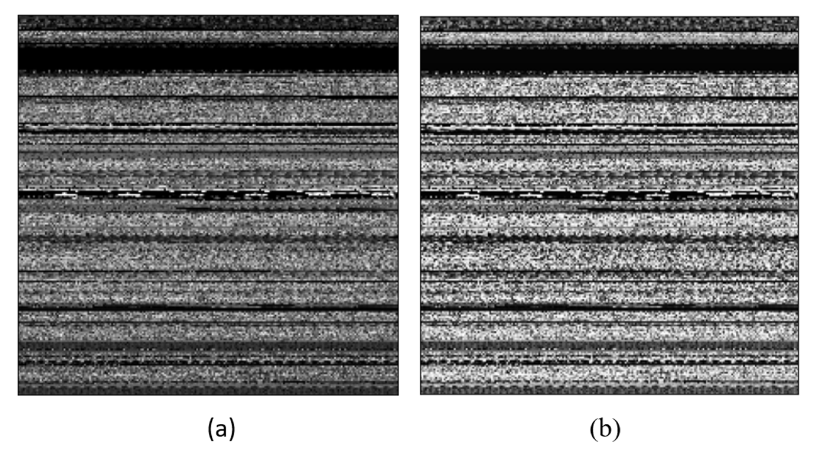
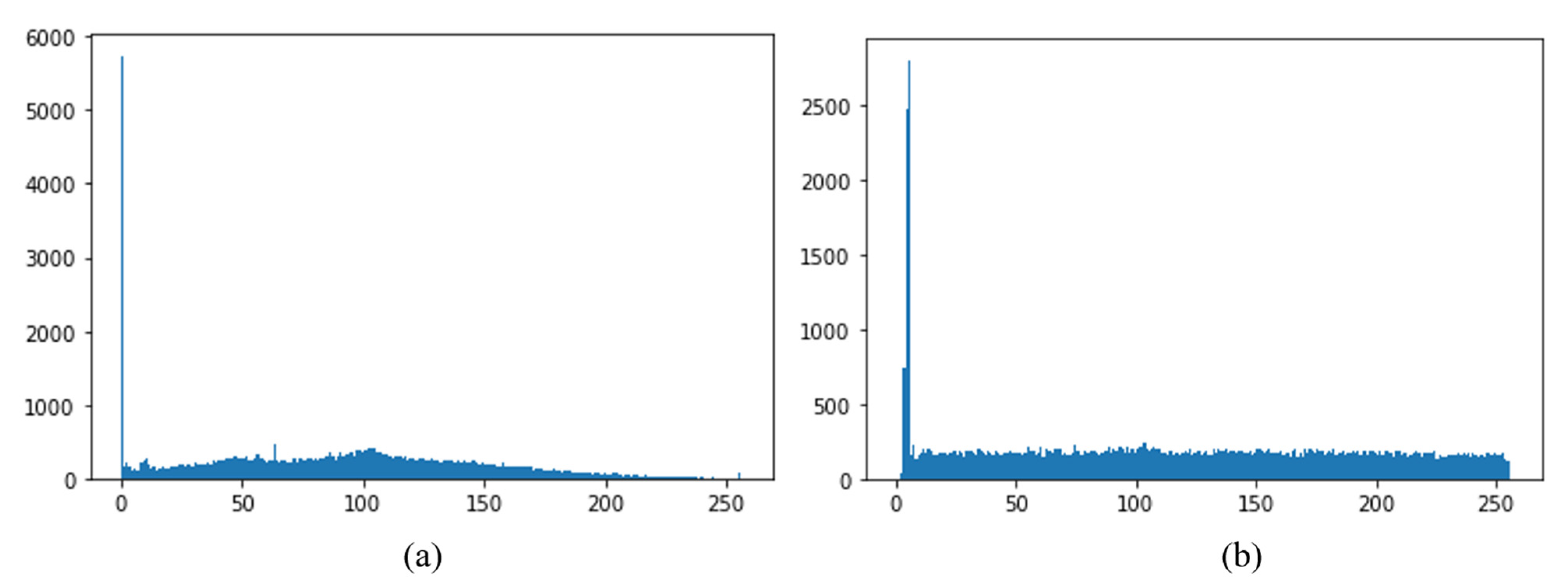
The image transformation yielded images of various classes with a variety of dimensions. We resized all images to 224 × 224 grayscale pixels by using the computer vision library without interpolation. The values of the grayscale images range from 0 to 255. A computer vision library was used to implement CLAHE on all images (CV2). Following this, we observed a slight shift in the pixel values of the images. Extremely dark pixels (0) became lighter while extremely bright pixels (255) became dark gray, indicating noise. The pywt module of Python was used to access features of the wavelet transform. All images were compressed to different levels throughout the process. We executed levels 1 and 2 of the wavelet transform on images with dimensions of 112 × 112 and 56 × 56, respectively. Hereinafter, we refer to these two tiers of datasets as version 1 and version 2, respectively. The files from the memory dump belonging to malware and benign programs are classified accordingly. We used five well-known machine learning classifiers: SVM with RBF, SVM with linear, RF, XGBoost, and the decision tree. The experiment began by training the machine learning classifiers on version 1 of the dataset. The same procedure was then used with version 2. The results of both versions were compared, and the performance of the best classifier was compared with the results of methods proposed in past work.

4.1. Notations and Preliminaries

In the past, accuracy as a performance metric was frequently used to evaluate any technique; however, this increases the likelihood of overfitting. We evaluated the technique based on its precision, recall, and F1-score. The ratio of true positives to the sum of true positives and false positives defines precision. It quantifies the number of false positives incorporated into the sample. If no false positives (FPs) occur, the model has an accuracy of 100%. The more FPs are added to the mix, the more imprecise the outcome. The positive and negative numbers from a confusion matrix were required to determine the accuracy of the model. Precision was calculated as follows:

Precision = TP/(TP + FP)

(1)

Rather than focusing on the number of false positives predicted by the model, recall considers the number of false negatives in the results of the prediction. The recall rate is penalized when a false negative is predicted because the penalties for precision and recall are the opposite. It is expressed as follows:

Recall = TP/(TP + FN)

(2)

The F1-score balances the accuracy and recall rate. The closer the F1-score is to 1, the better the classification. It is expressed as follows:

F1-score = 2 (Precision × Recall)/Precision + Recall

(3)

The confusion matrix was used to assess the performance of any given classification. It is an N × N matrix used to evaluate the performance of a classification model, where N is the number of target classes. The matrix compares values predicted by the model with the target values. It provides a comprehensive perspective on the performance of a classification model and the kinds of mistakes made.

4.2. Implementation and Results

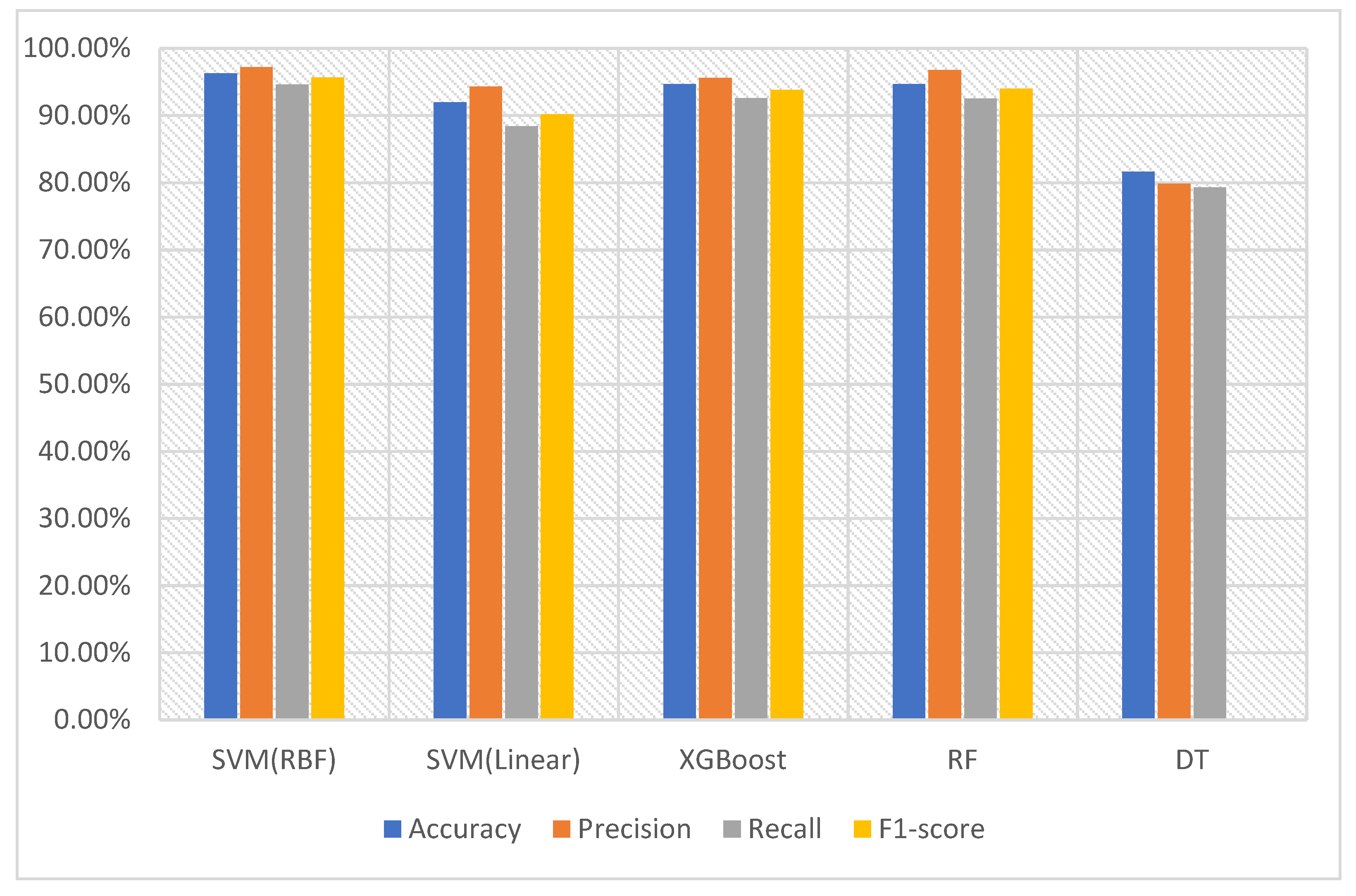
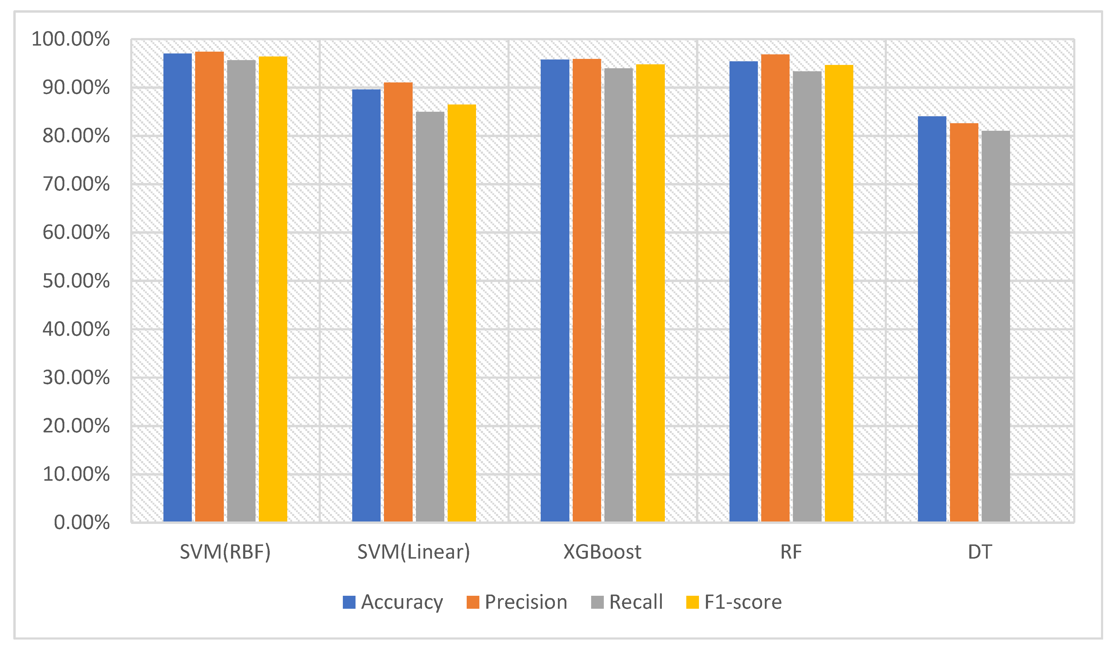
In order to feed data into the machine learning classifiers, we converted version 1 of the dataset of images into feature vectors. They were input to the SVM with RBF and the SVM with the linear kernel, XGBoost, RF, and DT. The SVM with the RBF kernel was able to recognize and classify the malware with an accuracy of 96.28%. Its scores of precision, recall, and F1-score were 97.17%, 94.62%, and 95.66%, respectively. This indicates that the SVM with the RBF kernel obtained a sufficient amount of information from the feature vectors to be able to differentiate between the malware and benign data. RF delivered the second-best performance with an accuracy of 94.66%, precision of 96.75%, recall of 94.50%, and F1-score of 94.02%. The results obtained using the version 1 dataset are depicted in

Table 7. Comparison of the results of the machine learning classifiers on version 1 of the dataset.

#	ML	Pixels Size	Feature	Level	Accuracy	Precision	Recall	F1-Score
1	SVM (RBF)	112 × 112	CLAHE + WT	L 1	96.28%	97.17%	94.62%	95.66%
2	SVM (Linear)	112 × 112	CLAHE + WT	L 1	91.94%	94.28%	88.39%	90.16%
3	XGBoost	112 × 112	CLAHE + WT	L 1	94.66%	95.62%	92.58%	93.78%
4	RF	112 × 112	CLAHE + WT	L 1	94.66%	96.75%	92.50%	94.02%
5	DT	112 × 112	CLAHE + WT	L 1	81.62%	79.84%	79.28%	79.48%

and Figure 10.

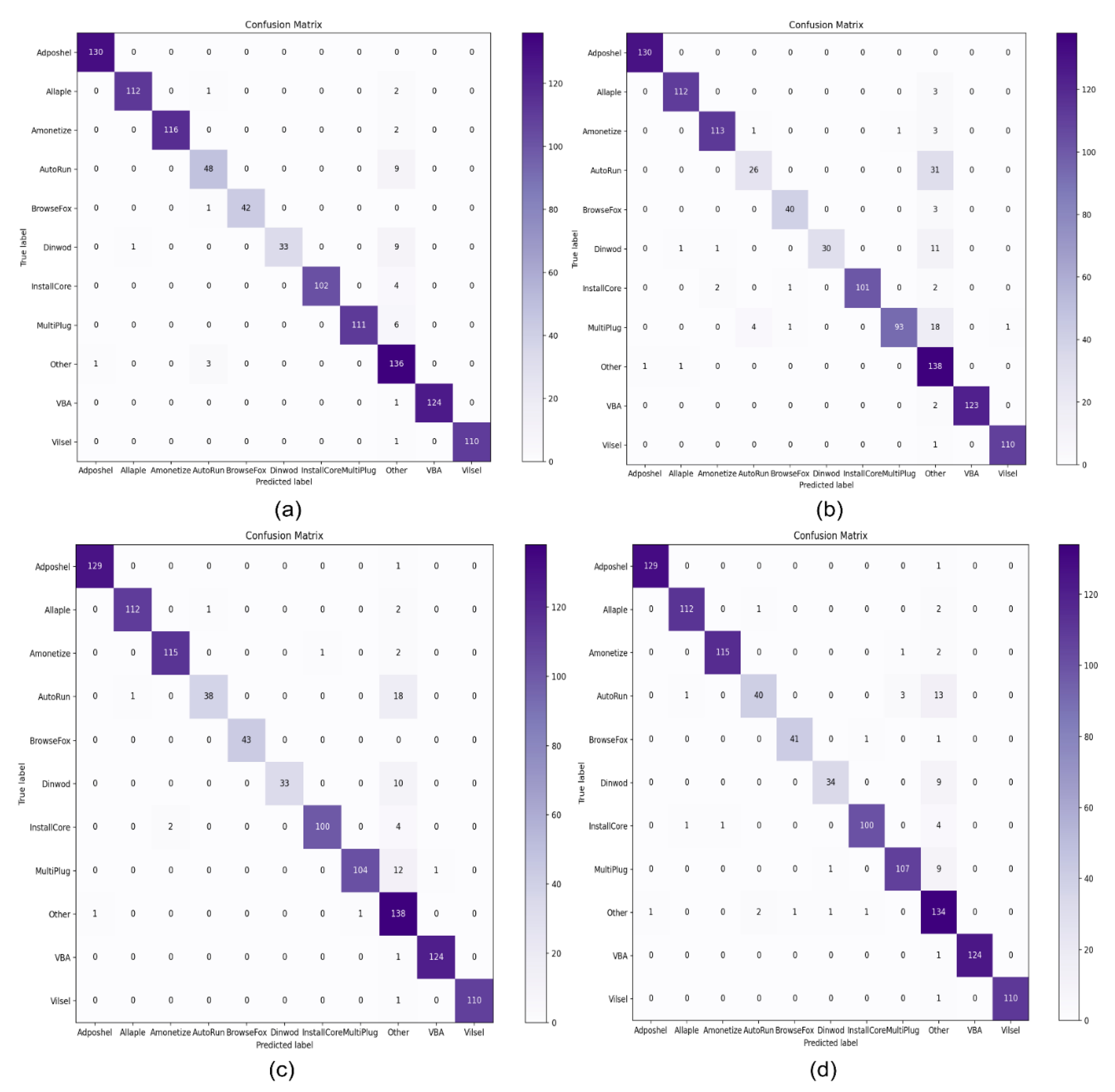
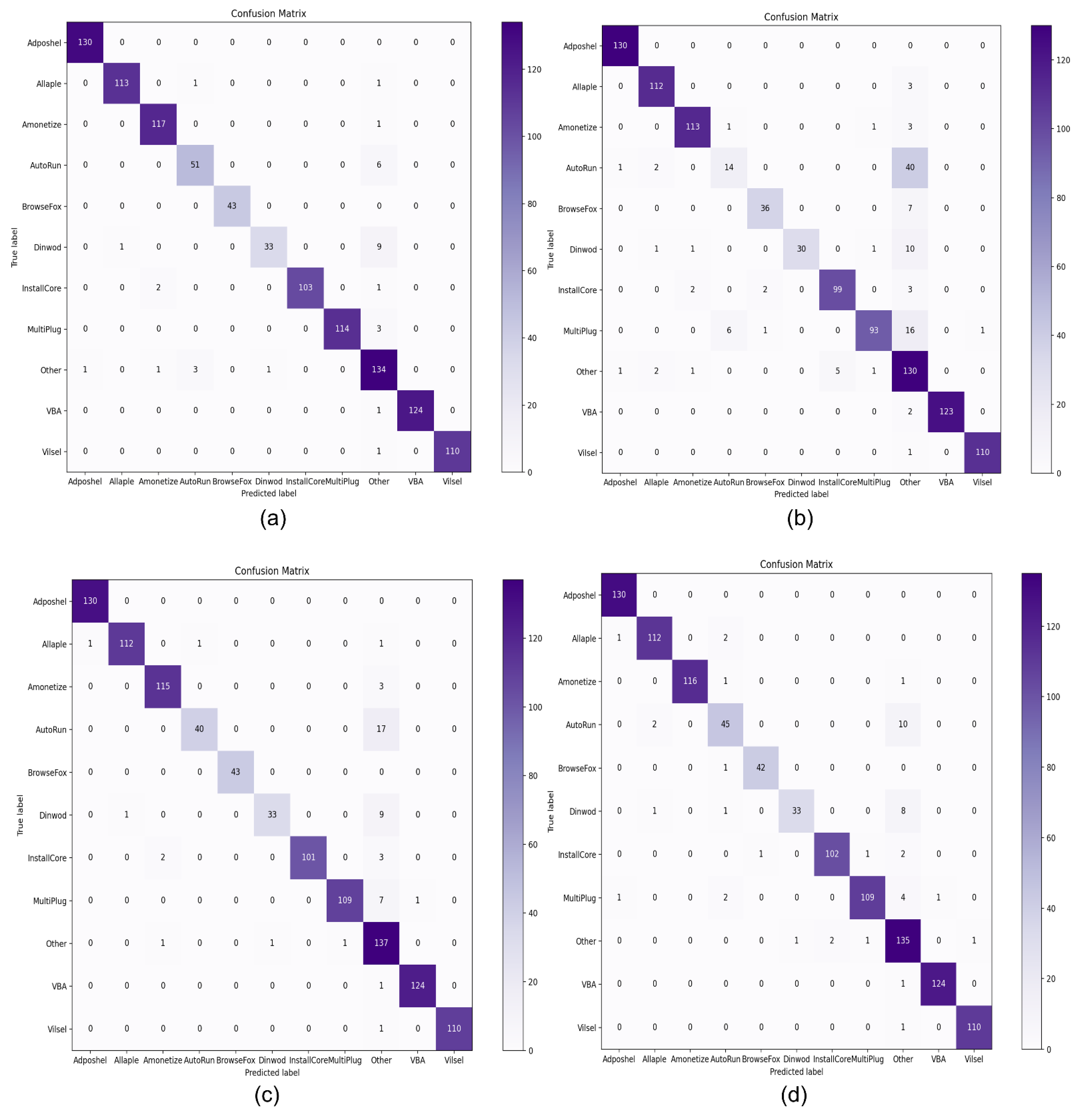
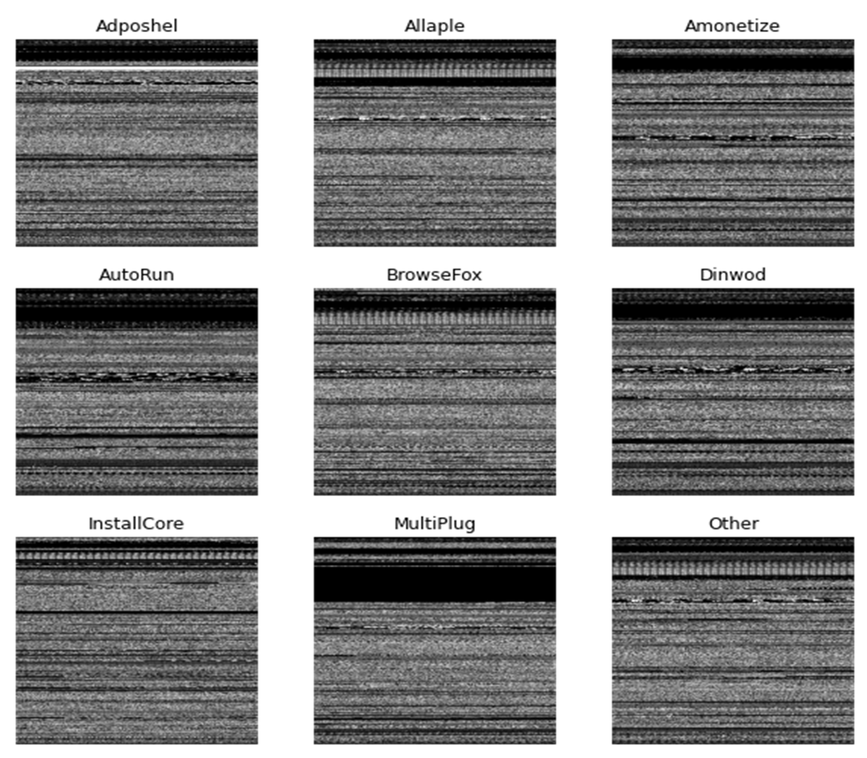
Figure 11 illustrates the confusion matrixes of the top four machine learning classifiers, including SVM with RBF, SVM with Linear, RF, XGBoost and DT. Among them is the SVM with the RBF classifier to highlight its performance in terms of identifying malware and benign software. Figure 11a shows that among the various malware classes, “Adposhel” achieved a 100% correct result, while “Dinwod” performed slightly worse, with a 95% classification rate. The proposed technique accurately classified benign images, as shown in the part of the diagram marked “other”. The use of CLAHE and wavelet transform for noise reduction and image compression enabled us to extract a sufficient number of useful features to successfully distinguish between the classes.

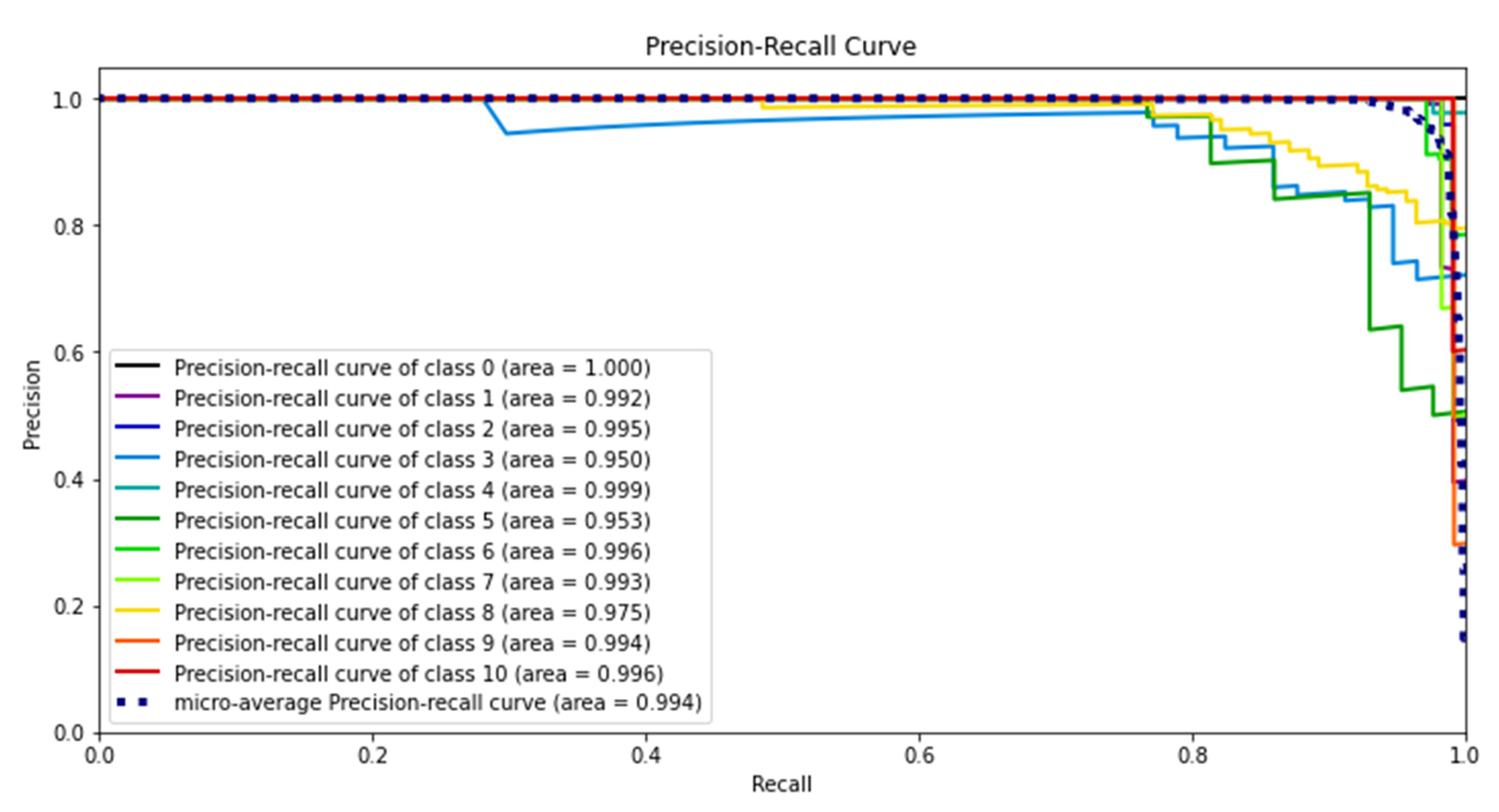
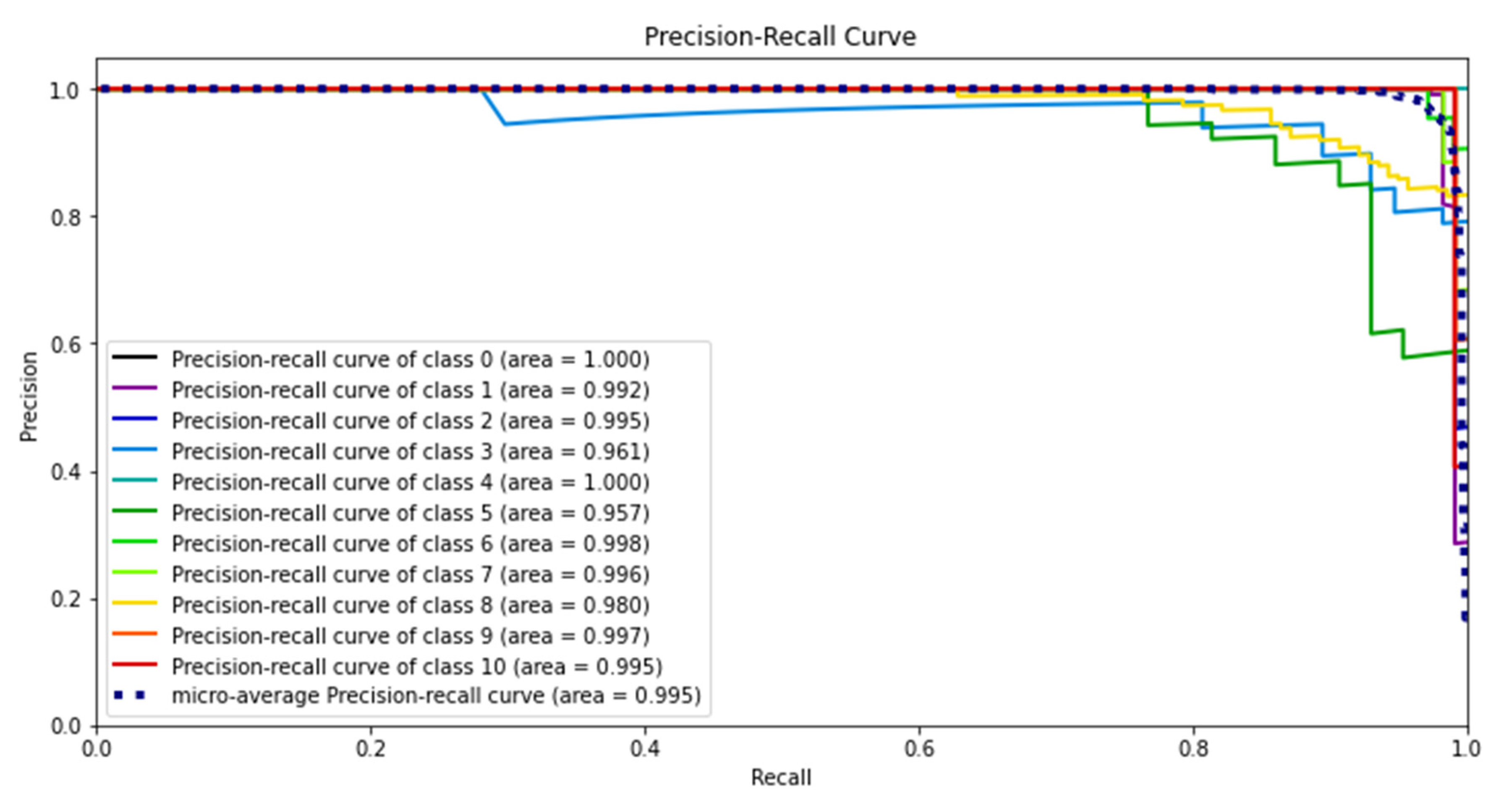
We also evaluated the performance of the best classifier in terms of the precision–recall curve (PRC). It illustrates the tradeoff between precision and recall when the threshold is changed. A large area under the curve indicates good recall and precision when the rates of false positives and false negatives are low. The higher the scores are, the more accurate the classifier (high precision), and the greater the number of positive results that it returns (high recall). Figure 12 depicts the results of the SVM with the RBF kernel classifier on various families of malware. The highest precision and recall values on version 1 are obtained for class 0 (Adposhel), with inferior performance on class 3 (AutoRun) and class 5 (Dinwod), and it is most probably due to the unbalanced dataset. We are optimistic about improving the performance of those worse malware family classes if applied to a balanced dataset. The overall value of the area of the PRC for various malware classes shows that the proposed technique worked well even on unbalanced datasets.

Memory utilization and time consumption during training are critical considerations in evaluating a given model or technique. We used a Python script to determine the computer’s memory utilization logs and the time taken for training. During the training phase, the SVM with the RBF kernel used 4090.3 MB of system memory and took 586 s. The XGBoost classifier consumed 3927.1 MB and took 519 s, whereas the DT had the lowest memory utilization and the shortest training time of 3880.0 MB and 72 s, respectively.

Table 8. Memory utilization of the machine learning classifiers on version 1 of the dataset.

S.No	Classifiers	Memory Usage (MB)
1	SVM-RBF	4090.3
2	SVM-Linear	4077.9
3	Random Forest	3892.3
4	XGBoost	3927.1
5	Decision Tree	3886.0

exhibits the experimental outcomes in terms of memory usage for all machine learning classifiers during training.

In the next experiment, we used version 2 of the dataset of memory-related images with dimensions of 56 × 56. The experiment was conducted with the same settings and classifiers. The SVM with the RBF kernel achieved the highest accuracy of 97.01%. The RF classifier, which delivered the second-best performance in terms of accuracy on version 1 of the dataset, now has lower accuracy, indicating that it did not obtain a sufficient amount of information to discriminate between different classes of malware. The XGBoost classifier achieved the second-highest accuracy of 95.74%. The performance of the classifiers is shown in

Table 9. Comparison of the results of the machine learning classifiers on version 2 of the dataset.

#	Classifiers	Pixels Size	Features	Level	Accuracy	Precision	Recall	F1-Score
1	SVM (RBF)	56 × 56	CLAHE + WT	L2	97.01%	97.36%	95.65%	96.36%
2	SVM (Linear)	56 × 56	CLAHE + WT	L2	89.59%	91.03%	84.94%	86.45%
3	XGBoost	56 × 56	CLAHE + WT	L2	95.74%	95.91%	93.92%	94.74%
4	RF	56 × 56	CLAHE + WT	L2	95.38%	96.84%	93.30%	94.62%
5	DT	56 × 56	CLAHE + WT	L2	83.98%	82.56%	80.99%	81.66%

and Figure 13 to be 97.36%

We used the confusion matrix of the top four machine learning classifiers in order to evaluate the performance of version 2 of the dataset. Among all machine learning classifiers, SVM with RBF kernel successfully classified various malware classes. Figure 14a shows its overall performance on various classes of malware. It attained the highest accuracy on the “Adposhel” class of malware, with a classification rate of 100%, but delivered slightly worse results on “Dinwod”. As shown in Figure 14a–d, the “AutoRun” class obtained the most confusing of the various confusion matrices of machine learning classifiers.

As shown in Figure 15, we used the PRC to determine how well the SVM with the RBF kernel performed on unbalanced classes of the dataset with fewer dimensions. When compared to version 1 of the dataset result, our technique improved almost classes of malware, such as class 3 (AutoRun), class 4 (BrowseFox), class 5 (Dinwod), class 6 (InstallCore), class 7 (MultiPlug), class 8 (other), class 9 (VBA), and class 10 (Vilsel). It was discovered that the wavelet transformer technique is capable of appropriately transforming non-stationary image signals and achieving both good frequency resolution for low-frequency images and high temporal resolution for high-frequency components.

Finally, we evaluated our classifiers in terms of memory utilization and time consumption during training.

Table 10. Memory utilization of the machine learning classifiers on version 2.

No	Classifiers	Memory Usage (MB)
1	SVM-RBF	2667.0
2	SVM-Linear	2673.1
3	Random Forest	2638.5
4	XGBoost	2644.4
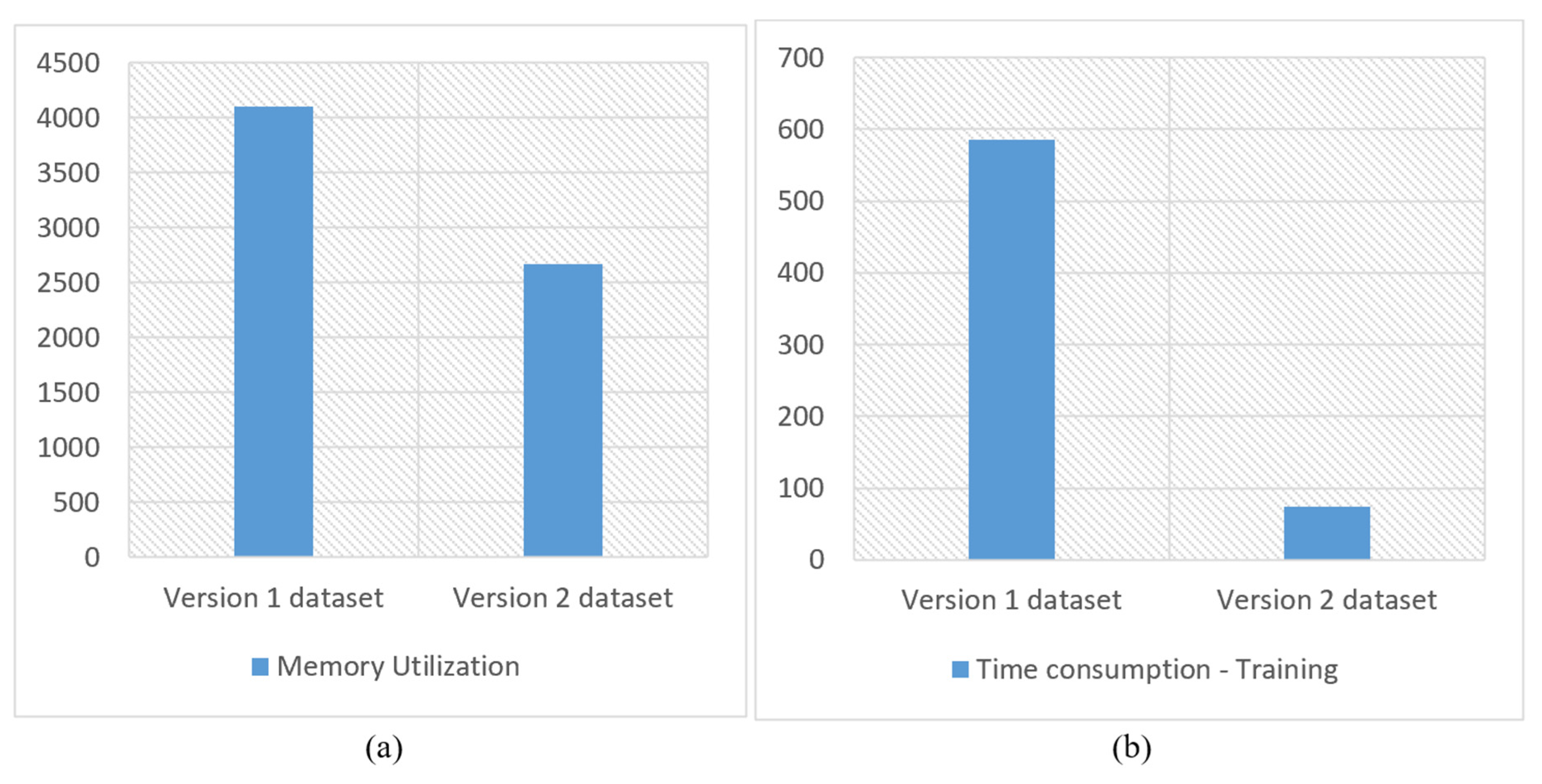
5	Decision Tree	2630.1

displays the overall memory usage during the training process. The SVM with the RBF kernel once again delivered the best performance, such as lower memory utilization from 4090.3 MB to 2667 MB and a training time from 586 s to 74 s without compromising the efficiency.

The proposed technique that uses CLAHE and the wavelet transform is able to reduce or eliminate noise in all memory-related images. It is also able to significantly compress the images to increase the accuracy of the SVM classifier while reducing the memory consumption and the cost of training the system. Our proposed method used images with 56 × 56 pixels, which is a significantly smaller size than what was considered in past studies. Finally, we compared the overall results of the proposed method with the state-of-the-art work reported in [14,15,16,18], as shown in

Table 11. Comparison of our proposed classifier with state-of-the-art methods.

Study	Accuracy	Precision	Recall	F1-Score
[14]	91.40%	91.50%	91.40%	91.50%
[18]	94.54%	94.60%	94.50%	94.50%
[15]	96.93%	97.00%	96.90%	96.90%
[16]	96.36%	96.40%	96.40%	96.40%
Proposed model	97.01%	97.36%	95.65%	96.36%

. The authors of [14] used GIST descriptors in conjunction with machine learning methods, while those of [18] applied HOG descriptors through a multi-layer perceptron model. Similarly, the authors of [15] recommended the use of deep convolutional neural networks via the VGG16 architecture, whereas the research in [16] utilized a combination of GIST and HOG for feature selection. A downside of GIST is that it divides images into parts by using a spatial grid [41], whereas the accuracy of HOG is unreliable due to its processing speed during object detection. The proposed technique relies on feature selection by using CLAHE and the wavelet transform. To compare our approach with the above methods, we used accuracy, precision, recall, and the F1-score as performance criteria. Our findings show that the proposed method outperformed all the others on each of the metrics, such as accuracy and precision. It is also able to identify elements in images with the smallest dimensions.

We compared the proposed method with the best classifiers on both datasets to evaluate its performance in terms of memory usage and training time and found that it delivered significant improvements in both. The SVM with the RBF kernel achieved the best performance on both versions of the dataset, and thus we compared its memory usage and training time/cost. Figure 16 shows that the use of CLAHE and the wavelet transform helped reduce memory utilization and training time.

5. Conclusions

Identifying and classifying various types of malware is very important especially in the existence of Advanced Persistent Threat (APT) because it provides information on how they infect computers or devices, the harm they can do to such systems, and ways to safeguard against them. In this paper, we proposed a memory-based technique to detect malware that are not easily being detected by the traditional malware detection techniques i.e., malware that resides in main computer memory. Feature extraction is the critical part in malware detection, and we used two techniques: CLAHE and the wavelet transform. Both techniques were able to extract features from the images in such a way that the machine learning classifiers that subsequently used them were able to recognize different types of malware and distinguish them from benign image files. The experimental results showed that our proposed technique is superior to prevalent methods in terms of accuracy and precision while using less memory and time for training and testing. In the future, we plan to use different approaches for feature selection to further improve the accuracy of the proposed method and reduce more its computational cost.