Phase Transition of Total Variation Based on Approximate Message Passing Algorithm

Abstract

In compressed sensing (CS), one seeks to down-sample some high-dimensional signals and recover them accurately by exploiting the sparsity of the signals. However, the traditional sparsity assumption cannot be directly satisfied in most practical applications. Fortunately, many signals-of-interest do at least exhibit a low-complexity representation with respect to a certain transformation. Particularly, total variation (TV) minimization is a notable example when the transformation operator is a difference matrix. Presently, many theoretical properties of total variation have not been completely explored, e.g., how to estimate the precise location of phase transitions and their rigorous understanding is still in its infancy. So far, the performance and robustness of the existing algorithm for phase transition prediction of TV model are not satisfactory. In this paper, we design a new approximate message passing algorithm to solve the above problems, called total variation vector approximate message passing (TV-VAMP) algorithm. To be specific, we first consider the problem from the Bayesian perspective, and formulate it as an optimization problem. Then, the vector factor graph for the TV model is constructed based on the formulized problem. Finally, the TV-VAMP algorithm is derived according to the idea of probabilistic inference in machine learning. Compared with the existing algorithm, our algorithm can be applied to a wider range of measurements distributions, including the non-zero-mean Gaussian distribution measurements matrix and ill-conditioned measurements matrix. Furthermore, in experiments with various settings, including different measurement distribution matrices, signal gradient sparsity, and measurement times, the proposed algorithm can almost reach the target mean squared error (−60 dB) with fewer iterations and better fit the empirical phase transition curve.

1. Introduction

Compressed sensing concerns the problem of recovering a high-dimensional signal ${\mathit{x}}^{☆}$ from a small number of linear observations $\mathit{y}$, which has received increasing attention over the past few years [1,2]. In recent years, compressed sensing has been applied to multifarious areas such as radar analysis, medical imaging, distributed signal processing, and data quantization, to name a few; see [3] for an overview. Similar to compressed sensing, the total variation model also belongs to the signal recovery model based on prior distribution. Since the TV model was proposed by Rudin [4], it has been applied in many fields due to its characteristics, such as image denoising [5] and compressed video sensing [6]. Especially, it plays a significant role in image restoration to recover signals from degraded measurements, such as denoising [7,8,9,10], compressed sensing [2,11], and deconvolution [12,13,14]. However, lots of theoretical properties of total variation regularization problems have not been explored [15], e.g., how to estimate the precise location of phase transitions is still an open problem [16,17].

Recent studies have shown that phase transitions occur in lots of stochastic convex optimization problems in mathematical signal processing and computational statistics [18,19]. In the case of random measurements, numerical results have observed that phase transitions emerge in total variation regularization problems. Concretely, when the number of the measurements exceeds a threshold, this procedure can precisely reconstruct signal ${\mathit{x}}^{☆}$ with high probability. When the number of the measurements is below the threshold, this procedure fails with high probability. This phenomenon is called phase transition [20]. Notably, the reason for studying phase transitions is to determine the minimum number of observations at which the original signal can be accurately recovered, which is meaningful in practical application.

Many related studies try to determine the location of this phase transition based on different proof strategies. For example, ref. [21] introduced the concept of $\mathit{D}$-RIP and has shown that $\mathcal{O}(s·\mathrm{Poly}(log(n/s))$ measurements are sufficient to guarantee success, where $s=\parallel \mathit{D}{\mathit{x}}^{☆}{\parallel }_0$ and $\mathit{D}$ denotes the TV operator. This bound on the sample rate naturally extends the classical guarantee for sparse recovery towards TV regularization. Another line of works [22,23,24] relied on Gaussian processing theory and demonstrated the phase transition occurs around ${\omega }^2({\mathcal{T}}_f\left({\mathit{x}}^{☆}\right)\cap {\mathbb{S}}^{n-1})$, where ${\mathcal{T}}_f\left({\mathit{x}}^{☆}\right)$ denotes the tangent cone introduced by $f(·)={\parallel \mathit{D}(·)\parallel }_1$ at point ${\mathit{x}}^{☆}$ and $\omega ({\mathcal{T}}_f\left({\mathit{x}}^{☆}\right)\cap {\mathbb{S}}^{n-1})$ represents the Gaussian width of the sphere part of this tangent cone. In contrast to [24], ref. [25] used tools from conical integral geometry and shown that the phase transition is located at $\delta \left({\mathcal{T}}_f\left({\mathit{x}}^{☆}\right)\right)$. Here $\delta \left({\mathcal{T}}_f\left({\mathit{x}}^{☆}\right)\right)$ denotes the statistical dimension of the same cone, which was proved to be almost equivalent to the squared Gaussian width; however, how to accurately estimate the Gaussian width or statistical dimension turns out to be a quite challenge problem. Several works have provided upper or lower bounds on these two geometric quantities. For example, ref. [26] established an upper bound on the Gaussian width when $\mathit{D}$ is a frame or TV operator. Ref. [27] improved this bound by using more careful approximations in the proofs. In a recent work [17], the authors obtained accurate estimation of ${\omega }^2({\mathcal{T}}_f\left({\mathit{x}}^{☆}\right)\cap {\mathbb{S}}^{n-1})$ when the Gram matrix $\mathit{D}{\mathit{D}}^T$ is almost diagonal. On the other hand, ref. [16] provided a numerically sharp lower bound for the statistical dimension when $\mathit{D}$ is TV operator; however, the results of above methods are only an approximation of the phase transition curve given from the perspective of the Gaussian process, and cannot fit the empirical phase transition accurately. In addition, they cannot give a specific solution to the problem.

Approximate message passing (AMP) algorithm is a kind of probability inference algorithm based on probability graph model in machine learning [28], which has been proved to be effective in reconstructing sparse signals from linear inverse problems [29,30,31]. It is worth noting that AMP algorithm is a general term for a class of probability inference algorithms, not a specific algorithm. Recently, some works study the phase transitions of total variation regularization problems under the approximate message passing (AMP) framework. Ref. [32] proposed a total variation approximate message passing (TVAMP) algorithm, attempted to solve the above problems and explore the phase transition of these problems at the same time; however, the TVAMP algorithm is limited to zero-mean Gaussian (or sub-Gaussian) measurements, and could not fit the empirical phase transition well.

In this paper, we follow a different strategy and provide a new iterative algorithm, total variation vector approximate message passing (TV-VAMP), to solve total variation regularization problems and estimate the phase transitions of these problems. The TVAMP algorithm in [32] is selected for comparison because it is an AMP-like approach as our algorithm, and provides a specific solution to total variation regularization problems. Numerical experiments verify that the proposed algorithm shows great advantage in many aspects. The main contributions made in our work are as follows:

• A new total variation vector approximate message passing algorithm (TV-VAMP) is designed to solve total variation regularization problems and estimate the phase transitions of these problems.
• Compared with the TVAMP algorithm, the proposed algorithm has better performance in convergence and phase transition prediction, when the measurements distribution is zero-mean Gaussian distribution.
• The proposed algorithm can be applied to a wider range of measurements distributions, including non-zero-mean measurements distribution and ill-conditioned measurements distribution, and has stronger robustness to the measurement matrix. In addition, TV-VAMP algorithm can still maintain excellent performance in the above scenarios.

The rest of this paper is organized as follows. In the next section, total variation regularization problems are expressed in the form of a mathematical formula. The specific derivation of the TV-VAMP algorithm for total variation model is discussed in Section 3. In Section 4, we make several numerical experiments and comparisons. Ultimately, Section 5 summarizes the entire work.

Before the discussion, the mathematical symbols in this paper are explained. Boldface letters in upper case and lower case denote matrices and column vectors, respectively. Scalars are signed with lowercase letters. Apart from that, the following mathematical symbols, parameters and operators are used:

• $tr$: the trace of a matrix;
• $\mathbb{R}$: the set of real numbers;
• ${∥·∥}_2$: Euclidean norm or ${\ell }_2$-norm;
• $\left|·\right|$: absolute-value norm or ${\ell }_1$-norm;
• ∂: differential operator;
• $y\propto x$: variable y is proportional to x;
• ${\mathit{A}}^{-1}$: inverse of matrix $\mathit{A}$;
• ${\mathit{A}}^T$: transpose of matrix $\mathit{A}$;
• $⟨\mathit{x},\mathit{y}⟩$: inner product of vector $\mathit{x}$ and vector $\mathit{y}$;
• $⟨\mathit{x}⟩$: the mean of the element-wise sums of the vector $\mathit{x}$;
• $diag(\mathit{x})$: a square diagonal matrix with the elements of vector $\mathit{x}$ on the main diagonal;
• $\mathbb{E}[\mathit{x}|f(\mathit{x})]$: the expectation of $\mathit{x}$ under the $f(\mathit{x})$ distribution;
• $Cov[\mathit{x}|f(\mathit{x})]$: the variance of $\mathit{x}$ under the $f(\mathit{x})$ distribution;
• $exp(·)$: simplified notation for exponential function;
• $\mathcal{N}\left(x;\mu ,\Sigma \right)$: variable x follows a Gaussian distribution with mean $\mu$ and variance $\Sigma$;
• $\mathrm{s}.\mathrm{t}.$: subject to.

2. Problem Formulations

The total variation model considers the problem of reconstructing a high-dimensional signal from a little collection of observations

$$\begin{array}{c}\hfill \mathit{y}=\mathit{A}{\mathit{x}}^{☆}+w,\end{array}$$

(1)

where $\mathit{A}\in {\mathbb{R}}^{m\times n}$ is a measurements matrix with $m<<n$ and $w\in {\mathbb{R}}^m$ represents the observation noise. The goal is to recover unknown signal ${\mathit{x}}^{☆}$ from observation $\mathit{y}\in {\mathbb{R}}^m$. Traditional compressed sensing usually assumes that ${\mathit{x}}^{☆}$ is sparse (or nearly sparse), which is often not satisfied in practice. A increasing number of applications concern the case that ${\mathit{x}}^{☆}$ is sparse with respect to some transformations [15,21,33,34]. As a typical example, total variation model aims to solve this kind of recovery problem when the transformation operator is a difference matrix. The key idea is to analyze signal ${\mathit{x}}^{☆}\in {\mathbb{R}}^n$ with a collection of vectors ${\mathit{d}}_1,\dots ,{\mathit{d}}_{n-1}\in {\mathbb{R}}^n$, i.e.,

$$\mathit{D}{\mathit{x}}^{☆}={(⟨{\mathit{d}}_1,{\mathit{x}}^{☆}⟩,\dots ,⟨{\mathit{d}}_{n-1},{\mathit{x}}^{☆}⟩)}^T\in {\mathbb{R}}^{n-1},$$

where

$$\begin{array}{c}\hfill \mathit{D}=\left(\begin{array}{ccccc}-1\hfill & 1& 0& \cdots & 0\\ 0\hfill & -1& 1& \cdots & 0\\ ⋮\hfill & ⋮& \ddots & \ddots & 0\\ 0\hfill & \cdots & 0& -1& 1\end{array}\right)\end{array}$$

(2)

denotes the TV operator (difference matrix). One may expect the transformed signal $\mathit{D}{\mathit{x}}^{☆}$ to be sparse (or nearly sparse); a natural method to recover the signal is the ${\ell }_1$-analysis minimization:

$$\begin{array}{c}\hfill \underset{\mathit{x}\in {\mathbb{R}}^n}{min}\left|\mathit{D}{\mathit{x}}^{☆}\right|,\mathrm{s}.\mathrm{t}.{\parallel \mathit{y}-\mathit{A}\mathit{x}\parallel }_2\le \delta ,\end{array}$$

(3)

where $\delta \ge 0$ reflects the noise level in terms of ${\ell }_2$-norm. Consequently, total variation regularization problems can be formulized as problem (3).

3. Total Variation Vector Approximate Message Passing Algorithm

In this section, we discuss our algorithm in detail. First of all, we introduce the vector factor graph and state the vector message-passing rules. Then, we construct the vector factor graph for TV model based on problem (3). Finally, we give the specific derivation of our TV-VAMP algorithm for total variation regularization problems.

3.1. Introduction of Vector Factor Graph

A factor graph is a bipartite graph that shows the decomposition of a function. In probability theory, factor graphs are used to represent the factorization of probability distribution functions, which can be efficiently computed by belief propagation algorithm [35,36,37]. The factor graph consists of variable nodes and factor nodes, where the factor nodes are functions of the variable nodes, representing the relationship between the variables [38,39]. Variable nodes and factor nodes are connected to each other through messages. It is worth mentioning that the message and the belief (mentioned below) are both probability distributions of variables. As a matter of fact, message passing is equivalent to computing the marginal probabilities of a variable. In the factor graph, the probability distribution of the high-dimensional signal is iteratively calculated through the process of message passing. A vector factor graph is a special kind of factor graph whose variable nodes are vectors.

In a vector factor graph, the message passing between variables follows certain rules, which are called vector message passing rules [40]. There are three rules for vector messaging, as shown in Figure 1. We present them here for the sake of discussion.

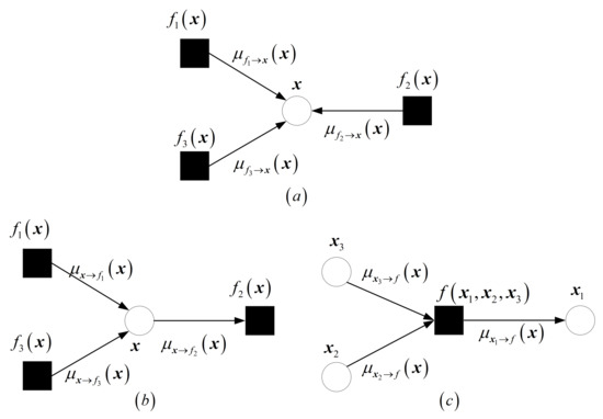
Figure 1. The figure illustrates vector message-passing rules. The circles represent variable nodes and the squares represent factor nodes. ${\mu }_{f\to \mathit{x}}(\mathit{x})$ denotes the message from the factor node f to the variable node $\mathit{x}$ and ${\mu }_{\mathit{x}\to f}(x)$ denotes the message from the variable node $x$ to the factor node f. (a) shows the rule of calculating approximate beliefs. (b) shows the rule of calculating variable-to-factor messages. (c) shows the rule of calculating factor-to-variable messages.

(1)

Approximate beliefs: The approximate belief on variable node $\mathit{x}$ is $b_{app}\left(\mathit{x}\right)\sim \mathcal{N}\left(\mathit{x};\widehat{\mathit{x}},\sigma \mathit{I}\right)$, where $\widehat{\mathit{x}}=\mathbb{E}\left[\mathit{x}\right|b_{sp}]$ and $\sigma =⟨diag(Cov\left[\mathit{x}\right|b_{sp}]⟩$ are the mean and average variance of the corresponding sum product belief $b_{sp}\left(\mathit{x}\right)\propto {\prod }_i{\mu }_{f_i\to \mathit{x}}\left(\mathit{x}\right)$. Illustration given by Figure 1a.

(2)

Variable-to-factor messages: The message from a variable node $\mathit{x}$ to a connected factor node $f_i$ is ${\mu }_{\mathit{x}\to f_i}\left(\mathit{x}\right)\propto b_{app}\left(\mathit{x}\right)/\phantom{b_{app}\left(\mathit{x}\right){\mu }_{f_i\to \mathit{x}}\left(\mathit{x}\right)}{\mu }_{f_i\to \mathit{x}}\left(\mathit{x}\right)$, i.e., the ratio of the most latest approximate belief $b_{app}\left(x\right)$ to the most recent message from $f_i$ to $\mathit{x}$. Illustration given by Figure 1b.

(3)

Factor-to-variable messages: The message from a factor node f to a connected variable node ${\mathit{x}}_i$ is ${\mu }_{f\to {\mathit{x}}_i}\left({\mathit{x}}_i\right)\propto \int f\left({\mathit{x}}_i,{\left\{{\mathit{x}}_j\right\}}_{j\ne i}\right){\prod }_{j\ne i}{\mu }_{{\mathit{x}}_j\to f}\left({\mathit{x}}_j\right)d{\mathit{x}}_j.$ See Figure 1c for an illustration.

3.2. Construction of Vector Factor Graph for TV Model

In Section 2, we obtain that total variation regularization problems can be formulized as problem (3). In this subsection, we consider the problem from a Bayesian perspective and further build relevant vector factor graph. Given a regularization parameter $\lambda \in \mathbb{R}$, the solution of problem (3) can be expressed as

$$\widehat{\mathit{x}}=\underset{x}{argmin}\frac{1}{2}{∥\mathit{y}-\mathit{A}\mathit{x}∥}_2^2+\lambda \left|\mathit{D}\mathit{x}\right|.$$

(4)

In accordance with maximum a posteriori probability (MAP) estimate, we give the following posterior distribution of $\mathit{x}$

$$p\left(\mathit{x}\right)\propto exp\left(-\lambda \left|\mathit{Dx}\right|\right)\mathcal{N}\left(\mathit{y};\mathit{Ax},{\gamma }_w^{-1}\mathit{I}\right)$$

(5)

and assume noise precision ${\gamma }_w\ge 0$. In fact, our estimate value $\widehat{\mathit{x}}$ is exactly the optimal value that maximizes the distribution $p\left(\mathit{x}\right)$ in Equation (5). Subsequently, we introduce a new variable $\mathit{z}=\mathit{Dx}$, giving an equivalent factorization

$$p\left(\mathit{x},\mathit{z}\right)\propto exp\left(-\lambda \left|\mathit{z}\right|\right)\delta \left(\mathit{z}-\mathit{Dx}\right)\mathcal{N}\left(\mathit{y};\mathit{Ax},{\gamma }_w^{-1}\mathit{I}\right),$$

(6)

where $\delta \left(·\right)$ is the Dirac delta distribution. In term of the joint distribution $p\left(\mathit{x},\mathit{z}\right)$, we could easily obtain the corresponding vector factor graph for total variation model, which is shown in Figure 2.

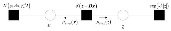
Figure 2. The figure shows the factor graph of Vector AMP for total variation regularization problems. The circles represent variable nodes and the squares represent factor nodes. ${\mu }_{\delta \to \mathit{x}}(\mathit{x})$ and ${\mu }_{\delta \to \mathit{z}}\left(\mathit{z}\right)$ denote the messages from the factor node $\delta \left(\mathit{z}-\mathit{Dx}\right)$ to the variable nodes $\mathit{x}$ and $\mathit{z}$. There are mutual messages between any two adjacent nodes in the graph. We omit some messages that are not drawn.

Consequently, the solution of problem (3) is equivalent to finding $\widehat{\mathit{x}}$ that maximizes the distribution $p\left(\mathit{x},\mathit{z}\right)$ in Equation (6). In the next subsection, we give the derivation of $\widehat{\mathit{x}}$ on the basis of the vector message-passing rules and vector factor graph for total variation model. Specifically, we first find the approximate distribution of $\mathit{x}$, then calculate the expectation of the distribution, which is the estimation of the real signal. Notably, the above steps are calculated iteratively through the message-passing process in Figure 2.

3.3. Derivation of TV-VAMP Algorithm

In this section, we present the detailed derivation of TV-VAMP algorithm. First of all, we assume that the messages from factor node $\delta \left(\mathit{z}-\mathit{Dx}\right)$ to variable nodes $\mathit{x}$ and $\mathit{z}$ are Gaussian distributions,

$${\mu }_{\delta \to \mathit{x}}(\mathit{x})\propto exp\left(-\frac{{\gamma }_1}{2}{\left(\mathit{Dx}\right)}^T\left(\mathit{Dx}\right)+{\gamma }_1{\mathit{r}}_1^T\left(\mathit{Dx}\right)\right),$$

(7)

$${\mu }_{\delta \to \mathit{z}}\left(\mathit{z}\right)\propto exp\left(-\frac{{\gamma }_2}{2}{\mathit{z}}^T\mathit{z}+{\gamma }_2{\mathit{r}}_2^T\mathit{z}\right).$$

(8)

After that, we initialize the message passing with

$${\mu }_{\delta \to \mathit{x}}\propto exp\left(-\frac{{\gamma }_{10}}{2}{(\mathit{Dx})}^T\mathit{Dx}+{\gamma }_{10}{\mathit{r}}_{10}^T\mathit{Dx}\right).$$

(9)

Throughout the derivation, k denotes the TV-VAMP iteration. The following steps are then repeated for $k=0,1,2,\dots ,K$. The concrete derivation of algorithm follows the steps below.

Step 1: Calculate approximate belief $b_{app}\left(\mathit{x}\right)$. Applying vector message passing rule 1 to the variable $\mathit{x}$ in Figure 2, we have

$$\begin{array}{cc}\hfill b_{sp}\left(\mathit{x}\right)& \propto {\mu }_{\delta \to \mathit{x}}(\mathit{x})\mathcal{N}\left(\mathit{y};\mathit{Ax},{\gamma }_w^{-1}\mathit{I}\right)\hfill \\ \hfill & \propto exp\left(-\frac{{\gamma }_{1k}}{2}{\left(\mathit{Dx}\right)}^T\left(\mathit{Dx}\right)+{\gamma }_{1k}{\mathit{r}}_{1k}^T\left(\mathit{Dx}\right)\right)\mathcal{N}\left(\mathit{y};\mathit{Ax},{\gamma }_w^{-1}\mathit{I}\right)\hfill \\ \hfill & =exp\left(-\frac{{\mathit{x}}^T\mathit{x}-2{\mathit{\xi }}^T{\Omega }^{-1}\mathit{x}}{2{\Omega }^{-1}}\right),\hfill \end{array}$$

(10)

where

$$\Omega ={\gamma }_w{\mathit{A}}^T\mathit{A}+{\gamma }_{1k}{\mathit{D}}^T\mathit{D},$$

(11)

$$\mathit{\xi }={\gamma }_w{\mathit{A}}^T\mathit{y}+{\gamma }_{1k}{\mathit{D}}^T{\mathit{r}}_{1k}.$$

(12)

Accordingly, the mean and average variance of the estimated value of variable $\mathit{x}$ in step k can be obtained for

$${\widehat{\mathit{x}}}_k={\left({\gamma }_w{\mathit{A}}^T\mathit{A}+{\gamma }_{1k}{\mathit{D}}^T\mathit{D}\right)}^{-1}\left({\gamma }_w{\mathit{A}}^T\mathit{y}+{\gamma }_{1k}{\mathit{D}}^T{\mathit{r}}_{1k}\right),$$

(13)

$${\left({\sigma }_{\mathit{x}}\right)}_k=\frac{1}{n}tr\left({\left({\gamma }_w{\mathit{A}}^T\mathit{A}+{\gamma }_{1k}{\mathit{D}}^T\mathit{D}\right)}^{-1}\right),$$

(14)

which yields

$$b_{app}\left(\mathit{x}\right)\sim \mathcal{N}\left(\mathit{x};{\widehat{\mathit{x}}}_k,{\left({\sigma }_{\mathit{x}}\right)}_k\mathit{I}\right).$$

(15)

Step 2: Update parameters ${\gamma }_{2k}$ and ${\mathit{r}}_{\mathbf{2}\mathit{k}}$. Applying vector message passing rule 2 to the variable $\mathit{x}$ in Figure 2, we have

$$\begin{array}{cc}\hfill {\mu }_{\mathit{x}\to \delta }\left(\mathit{x}\right)& =b_{app}\left(\mathit{x}\right)/\phantom{b_{app}\left(\mathit{Dx}\right){\mu }_{\delta \to \mathit{Dx}}(\mathit{Dx})}{\mu }_{\delta \to \mathit{x}}\left(\mathit{x}\right)\hfill \\ \hfill & =exp\left(-\frac{1}{2{\left({\sigma }_{\mathit{x}}\right)}_k}{\left(\mathit{x}-{\widehat{\mathit{x}}}_k\right)}^T\left(\mathit{x}-{\widehat{\mathit{x}}}_k\right)\right)/\phantom{exp\left(-\frac{1}{2{\left({\sigma }_{\mathit{x}}\right)}_k}{\left(\mathit{x}-{\widehat{\mathit{x}}}_k\right)}^T\left(\mathit{x}-{\widehat{\mathit{x}}}_k\right)\right){\mu }_{\delta \to \mathit{x}}\left(\mathit{x}\right)}{\mu }_{\delta \to \mathit{x}}\left(\mathit{x}\right)\hfill \\ \hfill & \approx exp\left(-\frac{1}{2{\left({\sigma }_{\mathit{Dx}}\right)}_k}{\left(\mathit{x}-{\widehat{\mathit{x}}}_k\right)}^T{\mathit{D}}^T\mathit{D}\left(\mathit{x}-{\widehat{\mathit{x}}}_k\right)\right)/\phantom{exp\left(-\frac{1}{2{\left({\sigma }_{\mathit{Dx}}\right)}_k}{\left(\mathit{x}-{\widehat{\mathit{x}}}_k\right)}^T{\mathit{D}}^T\mathit{D}\left(\mathit{x}-{\widehat{\mathit{x}}}_k\right)\right){\mu }_{\delta \to \mathit{x}}\left(\mathit{x}\right)}{\mu }_{\delta \to \mathit{x}}\left(\mathit{x}\right)\hfill \\ \hfill & =exp\left(-\frac{1}{2}{\phi }_{1k}{\left(\mathit{Dx}\right)}^T\left(\mathit{Dx}\right)+{\mathit{\nu }}_{1k}^T\left(\mathit{Dx}\right)\right),\hfill \end{array}$$

(16)

where

$${\left({\sigma }_{\mathit{Dx}}\right)}_k=\frac{1}{n}tr\left({\left({\gamma }_w{\mathit{A}}^T\mathit{A}+{\gamma }_{2k}{\mathit{D}}^T\mathit{D}\right)}^{-1}{\mathit{D}}^T\mathit{D}\right),$$

(17)

and

$${\phi }_{1k}=\frac{1}{{\left({\sigma }_{\mathit{Dx}}\right)}_k}-{\gamma }_{1k},$$

(18)

$${\mathit{\nu }}_{1k}=\frac{\mathit{D}{\widehat{\mathit{x}}}_k}{{\left({\sigma }_{\mathit{Dx}}\right)}_k}-{\gamma }_{1k}{\mathit{r}}_{1k}.$$

(19)

Applying vector message passing rule 3 to the message ${\mu }_{\delta \to \mathit{z}}\left(\mathit{z}\right)$ in Figure 2, we have

$$\begin{array}{cc}\hfill {\mu }_{\delta \to \mathit{z}}\left(\mathit{z}\right)& =\int \delta \left(\mathit{z}-\mathit{Dx}\right){\mu }_{\mathit{x}\to \delta }\left(\mathit{x}\right)dx\hfill \\ \hfill & =exp\left(-\frac{1}{2}{\phi }_{1k}{\mathit{z}}^T\mathit{z}+{\mathit{\nu }}_{1k}^T\mathit{z}\right).\hfill \end{array}$$

(20)

Comparing Equation (20) with (8), we have

$${\phi }_{1k}=\frac{1}{{\left({\sigma }_{\mathit{Dx}}\right)}_k}-{\gamma }_{1k}={\gamma }_{2k},$$

(21)

$${\mathit{\nu }}_{1k}=\frac{\mathit{D}{\widehat{\mathit{x}}}_k}{{\left({\sigma }_{\mathit{Dx}}\right)}_k}-{\gamma }_{1k}{\mathit{r}}_{1k}={\gamma }_{2k}{\mathit{r}}_{2k}.$$

(22)

Step 3: Calculate approximate belief $b_{app}\left(\mathit{z}\right)$. Applying vector message passing rule 1 to the variable $\mathit{z}$ in Figure 2, we have

$$\begin{array}{cc}\hfill b_{sp}\left(\mathit{z}\right)& \propto p_0\left(\mathit{z}\right){\mu }_{\delta \to \mathit{z}}\left(\mathit{z}\right)\hfill \\ \hfill & =exp\left(-\lambda \left|\mathit{z}\right|-\frac{1}{2}{\gamma }_{2k}{\mathit{z}}^T\mathit{z}+{\gamma }_{2k}{\mathit{r}}_{2k}^T\mathit{z}\right).\hfill \end{array}$$

(23)

Unfortunately, we cannot obtain the mean $\widehat{\mathit{z}}$ and average variance ${\sigma }_{\mathit{z}}$ of the estimated value of variable $\mathit{z}$ for the distribution $b_{sp}\left(\mathit{z}\right)$. Therefore, we consider instead a different distribution here

$$f_{sp}\left(\mathit{z}\right)=exp\left(-\beta \left(\lambda \left|\mathit{z}\right|+\frac{1}{2}{\gamma }_{2k}{\mathit{z}}^T\mathit{z}-{\gamma }_{2k}{\mathit{r}}_{2k}^T\mathit{z}\right)\right)$$

(24)

and take the limit $\beta \to \infty$, thus making the entire mass of the distribution concentrate around its mode. Then, according to the Laplace approximate method [41], we can easily obtain

$$\begin{array}{cc}\hfill {\widehat{\mathit{z}}}_k& \approx \underset{\beta \to \infty }{lim}\mathbb{E}\left[\mathit{z}\right|f_{sp}]\hfill \\ \hfill & =\underset{\mathit{z}}{argmin}\left(\lambda \left|\mathit{z}\right|+\frac{1}{2}{\gamma }_{2k}{\mathit{z}}^T\mathit{z}-{\gamma }_{2k}{\mathit{r}}_{2k}^T\mathit{z}\right)\hfill \\ \hfill & =\eta \left(r_{2k},\frac{\lambda }{{\gamma }_{2k}}\right),\hfill \end{array}$$

(25)

$$\begin{array}{c}\hfill {\left({\sigma }_{\mathit{z}}\right)}_k\approx ⟨Cov\left[\mathit{z}\right|f_{sp}]⟩={\gamma }_{2k}^{-1}⟨\nabla \eta \left({\mathit{r}}_{2k},\frac{\lambda }{{\gamma }_{2k}}\right)⟩,\end{array}$$

(26)

where $\eta \left(·\right)$ is soft thresholding function

$$\eta \left(r_i,\lambda /\phantom{\lambda \gamma }\gamma \right)=\left\{\begin{array}{cc}{r}_i-\lambda /\phantom{\lambda \gamma }\gamma \hfill & \mathrm{if}{r}_i\ge \lambda /\phantom{\lambda \gamma }\gamma ,\hfill \\ 0\hfill & \mathrm{if}\left|r_i\right|<\lambda /\phantom{\lambda \gamma }\gamma ,\hfill \\ r_i+\lambda /\phantom{\lambda \gamma }\gamma \hfill & \mathrm{if}{r}_i\le -\lambda /\phantom{\lambda \gamma }\gamma .\hfill \end{array}\right.$$

Therefore, we obtain

$$b_{app}\left(\mathit{z}\right)\sim \mathcal{N}\left(\mathit{z};{\widehat{\mathit{z}}}_k,{\left({\sigma }_{\mathit{z}}\right)}_k\mathit{I}\right).$$

(27)

Here we consider the reason why the approximation (Equation (25)) holds from a different perspective. If we treat $p_0\left(\mathit{z}\right)$ and ${\mu }_{\delta \to \mathit{z}}\left(\mathit{z}\right)$ as the prior and likelihood functions, then the distribution $b_{sp}\left(\mathit{z}\right)$ is the corresponding posterior distribution. Therefore, the mean of $b_{sp}\left(\mathit{z}\right)$ can be regarded as the Bayesian solution of the problem:

$$\begin{array}{c}\hfill \underset{z}{min}\frac{{\gamma }_{2k}}{2}{∥\mathit{z}-{\mathit{r}}_{2k}∥}_2^2+\lambda \left|\mathit{z}\right|.\end{array}$$

Similarly, the mean of $f_{sp}\left(\mathit{z}\right)$ is the maximum a posteriori probability (MAP) solution of this problem. Specifically, when we take the limit $\beta \to \infty$, the entire mass of the distribution $f_{sp}\left(\mathit{z}\right)$ concentrate around the value making the posterior distribution $b_{sp}\left(\mathit{z}\right)$ maximum, which is in line with the maximum a posteriori estimation. Consequently, we can consider the above process as utilizing the MAP solution to approximate the Bayesian solution of the same problem.

Step 4: Update parameters ${\gamma }_{1k}$ and ${\mathit{r}}_{\mathbf{1}\mathit{k}}$. Applying vector message passing rule 2 to the variable $\mathit{z}$ in Figure 2, we have

$$\begin{array}{cc}\hfill {\mu }_{\mathit{z}\to \delta }\left(\mathit{z}\right)& =b_{app}\left(\mathit{z}\right)/\phantom{b_{app}\left(\mathit{z}\right){\mu }_{\delta \to \mathit{z}}\left(\mathit{z}\right)}{\mu }_{\delta \to \mathit{z}}\left(\mathit{z}\right)\hfill \\ \hfill & \propto \mathcal{N}\left(\mathit{z};{\widehat{\mathit{z}}}_k,{\left({\sigma }_{\mathit{z}}\right)}_k\mathit{I}\right)/\phantom{\mathcal{N}\left(\mathit{z};{\widehat{\mathit{z}}}_k,{\left({\sigma }_z\right)}_k\mathit{I}\right)exp\left(-\frac{{\gamma }_2}{2}{\mathit{z}}^T\mathit{z}+{\gamma }_2{\mathit{r}}_2^T\mathit{z}\right)}exp\left(-\frac{{\gamma }_{2k}}{2}{\mathit{z}}^T\mathit{z}+{\mathit{\gamma }}_{2k}{\mathit{r}}_{2k}^T\mathit{z}\right)\hfill \\ \hfill & =exp\left(-\frac{1}{2}{\phi }_{2k}{\mathit{z}}^T\mathit{z}+{\mathit{\nu }}_{2k}^T\mathit{z}\right),\hfill \end{array}$$

(28)

where

$${\phi }_{2k}=\frac{1}{{\left({\sigma }_{\mathit{z}}\right)}_k}-{\gamma }_{2k},$$

(29)

$${\mathit{\nu }}_{2k}=\frac{{\widehat{\mathit{z}}}_k}{{\left({\sigma }_{\mathit{z}}\right)}_k}-{\gamma }_{2k}{\mathit{r}}_{2k}.$$

(30)

Applying vector message passing rule 3 to the message ${\mu }_{\delta \to \mathit{x}}\left(\mathit{x}\right)$ in Figure 2, we have

$$\begin{array}{cc}\hfill {\mu }_{\delta \to \mathit{x}}\left(\mathit{x}\right)& =\int \delta \left(\mathit{z}-\mathit{Dx}\right){\mu }_{\mathit{z}\to \delta }\left(\mathit{z}\right)d\mathit{z}\hfill \\ \hfill & ={\mu }_{\mathit{z}\to \delta }(\mathit{Dx})\hfill \\ \hfill & =exp\left(-\frac{1}{2}{\gamma }_{2k}{(\mathit{Dx})}^T(\mathit{Dx})+{\gamma }_{2k}{\mathit{r}}_{2k}^T(\mathit{Dx})\right).\hfill \end{array}$$

(31)

Comparing Equation (31) with (7), we have

$${\phi }_{2k}=\frac{1}{{\left({\sigma }_{\mathit{z}}\right)}_k}-{\gamma }_{2k}={\gamma }_{1,k+1},$$

(32)

$${\mathit{\nu }}_{2k}=\frac{{\widehat{\mathit{z}}}_k}{{\left({\sigma }_{\mathit{z}}\right)}_k}-{\gamma }_{2k}{\mathit{r}}_{2k}={\gamma }_{1,k+1}{\mathit{r}}_{1,k+1}.$$

(33)

The above steps are then repeated with $k\leftarrow k+1$. Due to the parameters ${\gamma }_{1k},{\mathit{r}}_{1k}$ And ${\gamma }_{2k},{\mathit{r}}_{2k}$ are mutually expressed, so we can unify the parameters ${\gamma }_{1k},{\mathit{r}}_{1k}$ And ${\gamma }_{2k},{\mathit{r}}_{2k}$. To be specific, we define

$${\gamma }_k\equiv {\gamma }_{1k},{\mathit{r}}_k\equiv {\mathit{r}}_{1k}.$$

(34)

Then, according to Equations (21), (22), (32), and (33), we can obtain

$${\gamma }_{k+1}={\gamma }_{1,k+1}=\frac{1}{{\left({\sigma }_{\mathit{z}}\right)}_k}-{\gamma }_{2k}=\frac{1}{{\left({\sigma }_{\mathit{z}}\right)}_k}-\frac{1}{{\left({\sigma }_{\mathit{Dx}}\right)}_k}+{\gamma }_k,$$

(35)

and

$${\mathit{r}}_{k+1}={\mathit{r}}_{1,k+1}=\frac{\widehat{\mathit{z}}}{{\left({\sigma }_{\mathit{z}}\right)}_k}-{\mathit{r}}_{2k}=\frac{\widehat{\mathit{z}}}{{\left({\sigma }_{\mathit{z}}\right)}_k}-\frac{\mathit{D}{\widehat{\mathit{x}}}_k}{{\left({\sigma }_{\mathit{Dx}}\right)}_k}+{\mathit{r}}_k.$$

(36)

Furthermore, we have

$${\gamma }_{2k}=-\frac{1}{{\left({\sigma }_{\mathit{Dx}}\right)}_k}+{\gamma }_k,$$

(37)

and

$${\mathit{r}}_{2k}=-\frac{\mathit{D}{\widehat{\mathit{x}}}_k}{{\left({\sigma }_{\mathit{Dx}}\right)}_k}+{\mathit{r}}_k.$$

(38)

Subsequently, the approximate mean ${\widehat{\mathit{z}}}_k$ and average variance ${\left({\sigma }_{\mathit{z}}\right)}_k$ of the estimated value of the distribution $b_{sp}\left(\mathit{z}\right)$ in Equations (25) and (26) can be expressed as

$${\widehat{\mathit{z}}}_k=\eta \left(\frac{-\mathit{D}{\widehat{\mathit{x}}}_k+{\left({\sigma }_{\mathit{Dx}}\right)}_k{\mathit{r}}_k}{{\left({\sigma }_{\mathit{Dx}}\right)}_k},\frac{\lambda {\left({\sigma }_{\mathit{Dx}}\right)}_k}{{\left({\sigma }_{\mathit{Dx}}\right)}_k{\gamma }_k-1}\right),$$

(39)

and

$${\left({\sigma }_{\mathit{z}}\right)}_k=\frac{{\left({\sigma }_{\mathit{Dx}}\right)}_k}{{\left({\sigma }_{\mathit{Dx}}\right)}_k{\gamma }_k-1}⟨\partial \eta \left(\frac{-\mathit{D}{\widehat{\mathit{x}}}_k+{\left({\sigma }_{\mathit{Dx}}\right)}_k{\mathit{r}}_k}{{\left({\sigma }_{\mathit{Dx}}\right)}_k},\frac{\lambda {\left({\sigma }_{\mathit{Dx}}\right)}_k}{{\left({\sigma }_{\mathit{Dx}}\right)}_k{\gamma }_k-1}\right)⟩.$$

(40)

Finally, combining Equations (39), (40) with (13), (17), (35), and (36), we could obtain Algorithm 1. The output of our algorithm is ${\widehat{\mathit{x}}}_K$, which is the solution to problem (3), i.e., the estimated value of the true signal. Additionally, the other quantities in the algorithm are intermediate parameters.

Algorithm 1 TV-VAMP Algorithm

Require:  Matrix $\mathit{A}\in {\mathbb{R}}^{m\times n}$; measurements $\mathit{y}\in {\mathbb{R}}^m$; TV operator $\mathit{D}\in {\mathbb{R}}^{(n-1)\times n}$; assumed noise precision ${\gamma }_w\ge 0$; ${\gamma }_0=1$ and ${\mathit{r}}_0=\mathbf{0}$ ; number of iterations K. 1: for$k=0,1,2,\cdots ,K$do 2:    ${\widehat{\mathit{x}}}_k={\left({\gamma }_w{\mathit{A}}^T\mathit{A}+{\gamma }_k{\mathit{D}}^T\mathit{D}\right)}^{-1}\left({\gamma }_w{\mathit{A}}^T\mathit{y}+{\gamma }_k{\mathit{D}}^T{\mathit{r}}_k\right)$ 3:     4:    ${\left({\sigma }_{\mathit{Dx}}\right)}_k=\frac{1}{n}tr\left({\left({\gamma }_w{\mathit{A}}^T\mathit{A}+{\gamma }_k{\mathit{D}}^T\mathit{D}\right)}^{-1}{\mathit{D}}^T\mathit{D}\right)$ 5:     6:    ${\widehat{\mathit{z}}}_k=\eta \left(\frac{-\mathit{D}{\widehat{\mathit{x}}}_k+{\left({\sigma }_{\mathit{Dx}}\right)}_k{\mathit{r}}_k}{{\left({\sigma }_{\mathit{Dx}}\right)}_k},\frac{\lambda {\left({\sigma }_{\mathit{Dx}}\right)}_k}{{\left({\sigma }_{\mathit{Dx}}\right)}_k{\gamma }_k-1}\right))$ 7:     8:    ${\left({\sigma }_{\mathit{z}}\right)}_k=\frac{{\left({\sigma }_{\mathit{Dx}}\right)}_k}{{\left({\sigma }_{\mathit{Dx}}\right)}_k{\gamma }_k-1}⟨\partial \eta \left(\frac{-\mathit{D}{\widehat{\mathit{x}}}_k+{\left({\sigma }_{\mathit{Dx}}\right)}_k{\mathit{r}}_k}{{\left({\sigma }_{\mathit{Dx}}\right)}_k},\frac{\lambda {\left({\sigma }_{\mathit{Dx}}\right)}_k}{{\left({\sigma }_{\mathit{Dx}}\right)}_k{\gamma }_k-1}\right)⟩$ 9:     10:    ${\gamma }_{k+1}=\frac{1}{{\left({\sigma }_{\mathit{z}}\right)}_k}-\frac{1}{{\left({\sigma }_{\mathit{Dx}}\right)}_k}+{\gamma }_k$ 11:     12:    ${\mathit{r}}_{k+1}=\frac{{\widehat{\mathit{z}}}_k}{{\left({\sigma }_z\right)}_k}-\frac{\mathit{D}{\widehat{\mathit{x}}}_k}{{\left({\sigma }_{\mathit{Dx}}\right)}_k}+{\mathit{r}}_k$ 13: end for 14: Return ${\widehat{\mathit{x}}}_K$.

4. Simulation Results

In this section, we present several numerical experiments to compare the TV-VAMP algorithm with the TVAMP algorithm from [32]. We concern three different measurements matrices in this section:

• Zero-mean Gaussian distribution measurements matrix.
• Non-zero-mean Gaussian distribution measurements matrix.
• Ill-conditioned measurements matrix.

Furthermore, we discuss two types of simulation results for each measurements matrix:

• Normalized mean squared error (NMSE) convergence over iterations.
• Phase transitions.

Before the description, experimental settings are stated.

4.1. Experimental Settings

All these simulation results are averaged over 50 trials using the Monte Carlo method. At each Monte Carlo trial, we reconstruct unknown signal ${\mathit{x}}^{☆}\in {\mathbb{R}}^n$ from measurements $\mathit{y}\in {\mathbb{R}}^m$, where ${\mathit{x}}^{☆}$ is gradient sparse, noise $w\sim \mathcal{N}\left(\mathbf{0},{\gamma }_w^{-1}\mathit{I}\right)$ and noise precision ${\gamma }_w^{-1}={10}^{-8}$. Moreover, we consider that the transformation operator is a difference matrix in all experiments. For the TVAMP algorithm and TV-VAMP algorithm, we set the maximum iteration step to 500, and regularization parameter $\lambda =0.05$.

4.1.1. Experimental Settings for NMSE Convergence over Iterations Experiment

The experiment settings for NMSE convergence over iterations experiment are as follows: signal feature dimension $n=200$, m denotes the number of measurements times and s denotes signal gradient sparsity. We observe NMSE over iterations for four different scenarios of $(s,m)$:

(a)

$s=10$, $m=50$

(b)

$s=20$, $m=80$

(c)

$s=40$, $m=140$

(d)

$s=60$, $m=160$.

4.1.2. Experimental Settings for Phase Transition Experiment

The experiment settings for phase transition experiment are as follows: signal feature dimension $n=200$, the measurements number m and gradient sparsity s changes from 5 to n with step 5. We declare success if the solution to problem (3) satisfies

$$\frac{{∥\widehat{\mathit{x}}-{\mathit{x}}^{☆}∥}_2^2}{{∥{\mathit{x}}^{☆}∥}_2^2}\le {10}^{-6},$$

(41)

where ${\mathit{x}}^{☆}$ denotes the true value and $\widehat{\mathit{x}}$ denotes the estimated value.

4.2. Zero-Mean Gaussian Distribution Measurements Matrix A

In the first experiment, realizations of $\mathit{A}$ are constructed by drawing an i.i.d. $\mathcal{N}\left(\mu ,1/m\right)$ matrix and $\mu =0$. We have two tasks here.

4.2.1. NMSE Convergence over Iterations

First of all, we compare the convergence over iterations of TVAMP algorithm with TV-VAMP algorithm. The experimental results are shown in Figure 3.

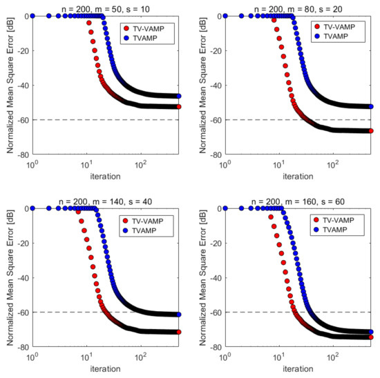
Figure 3. Normalized mean squared error (NMSE) convergence over iterations when $\mathit{A}$ is a zero-mean Gaussian distribution measurements matrix. Each curve is the average of 50 Monte Carlo samples.

Table 1 reports the results of the TVAMP algorithm and TV-VAMP algorithm when $\mathit{A}$ is a zero-mean Gaussian distribution measurements matrix. We give the number of iteration steps required for both algorithms to reach the target MSE (−60 dB of NMSE) in all cases. In four different experimental settings, our TV-VAMP algorithm can converge to the target MSE in the latter three cases, while TVAMP algorithm can only converge to the target MSE in the latter two cases. Additionally, we need fewer iteration steps and can converge to a smaller NMSE. Overall, our algorithm performs better in terms of convergence performance in this scenario.

Table 1. Average number of iterations to achieve NMSE = −60 dB for zero-mean Gaussian distribution measurements matrix.

Cases	$\mathit{s}=10,\mathit{m}=50$	$\mathit{s}=20,\mathit{m}=80$	$\mathit{s}=40,\mathit{m}=140$	$\mathit{s}=60,\mathit{m}=160$
TVAMP	∞	∞	112	36
TV-VAMP	∞	32	23	21

According to Table 1, we find that TVAMP and TV-VAMP algorithms cannot converge to the target MSE (−60 dB of NMSE) under some experimental settings. We believe that it is caused by insufficient measurement times. Notably, this is the purpose of our study of phase transition, which is discussed in the following section. We can determine the minimum number of measurements at which the real signal can be reconstructed according to the phase transition curve, which is of great significance in practical applications.

4.2.2. Phase Transition

In this subsection, we utilize TVAMP algorithm and TV-VAMP algorithm to predict the phase transition of total variation regularization problems. The purpose of studying phase transitions is to evaluate how the measurements number m varies with gradient sparsity s. Moreover, we can determine the minimum number of observations at which the original signal can be reconstructed.

In order to obtain the empirical phase transition, we use CVX [42] to solve the convex problem (3), which is a Matlab software for disciplined convex programming. Similarly, the empirical phase transition is averaged over 50 trials using the Monte Carlo method. The phase transition diagrams of CVX, TVAMP algorithm, and TV-VAMP algorithm, are shown in Figure 4.

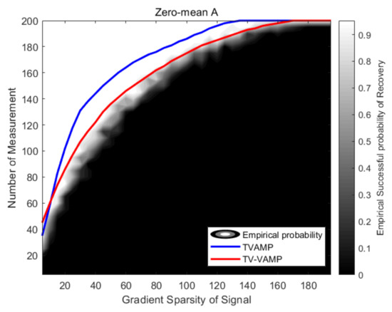
Figure 4. The figure shows phase transitions of CVX, TVAMP algorithm, and TV-VAMP algorithm when $\mathit{A}$ is a zero-mean Gaussian distribution measurements matrix and $n=200$.

The brightness of figure in each pair $(s,m)$ shows the empirical probability of success (black = 0% and white = 100%) in Figure 4. For the TVAMP algorithm and TV-VAMP algorithm, the phase transition curves are connection of experimental points having 0.5 success rate of the signal recovery. The upper part of the curve can reconstruct the original signal, while the part below the curve cannot. Compared with TVAMP algorithm, we can see that the phase transition curve obtained by TV-VAMP algorithm can better fit the empirical phase transition.

4.3. Non-Zero-Mean Gaussian Distribution Measurements Matrix A

In the second experiment, realizations of $\mathit{A}$ are constructed by drawing an i.i.d. $\mathcal{N}\left(\mu ,1/m\right)$ matrix and $\mu =1$. In a similar way, we have two different experiments here.

4.3.1. NMSE Convergence over Iterations

Firstly, the convergence of two different algorithms is compared. Our numerical experiment results are shown in Figure 5.

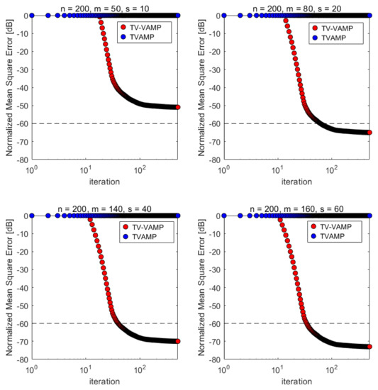
Figure 5. Normalized mean squared error (NMSE) convergence over iterations in the case of $\mu =1$ and $n=200$. Each curve is the average of 50 Monte Carlo samples.

Additionally, the results of two different algorithms are listed in Table 2 when $\mathit{A}$ is a non-zero-mean Gaussian distribution measurements matrix and the mean of the distribution $\mu =1$. Homogeneously, we give the number of iteration steps required to reach the target MSE (−60 dB of NMSE). Specifically, our TV-VAMP algorithm can converge to the target MSE in the latter three cases, while TVAMP algorithm all fails, which confirms the effectiveness of TV-VAMP algorithm.

Table 2. Average number of iterations to achieve NMSE = −60 dB for non-zero-mean Gaussian distribution measurements matrix.

Cases	$\mathit{s}=10,\mathit{m}=50$	$\mathit{s}=20,\mathit{m}=80$	$\mathit{s}=40,\mathit{m}=140$	$\mathit{s}=60,\mathit{m}=160$
TVAMP	∞	∞	∞	∞
TV-VAMP	∞	58	35	32

4.3.2. Phase Transition

In this subsection, since the TVAMP algorithm does not converge, we only compare the phase transition of TV-VAMP algorithm with the empirical phase transition. Equally, we use CVX [42] to obtain the empirical phase transition, and the experiment settings are the same as Section 4.2.2. The simulation results are shown in Figure 6. Conspicuously, the phase transition curve of TV-VAMP algorithm is still sufficiently close to the empirical phase transition when $\mathit{A}$ is a non-zero-mean Gaussian distribution measurements matrix.

Figure 6. The figure shows phase transitions of CVX and TV-VAMP algorithm in the case of $\mu =1$ and $n=200$.

4.4. Ill-Conditioned Measurements Matrix A

In the third experiment, we explore algorithm robustness to the condition number of $\mathit{A}$. In this case, realizations of $\mathit{A}$ are constructed from singular value decomposition (SVD) $\mathit{A}=\mathit{U}diag\left(\mathit{s}\right){\mathit{V}}^T$, where $\mathit{U}$ and $\mathit{V}$ are randomly sampled from the set of orthogonal matrices, and $\mathit{s}\in {\mathbb{R}}^m$ is constructed by singular values of $\mathit{A}$. We consider zero-mean measurements, i.e., $\mu =0$, and set $k(\mathit{A})=500$, where $k(\mathit{A})$ is the condition number of $\mathit{A}$, which is the ratio of the largest singular value to the smallest singular value of $\mathit{A}$.

4.4.1. NMSE Convergence over Iterations

First of all, we compare the convergence over iterations of two different algorithms. Figure 7 and Table 3 shows the results of two different algorithms when $\mathit{A}$ is ill-conditioned. Similarly, Table 3 reports the number of iteration steps required to reach the target MSE (−60 dB of NMSE). In four different experimental settings, our TV-VAMP algorithm can converge to the target MSE in the latter two scenarios, while the TVAMP algorithm is divergent in all experiments, which demonstrates the robustness of our algorithm. We believe that the reason why the NMSE of the TV-VAMP algorithm can not converge to −60 dB in the first two scenarios is that the number of measurements times are not enough.

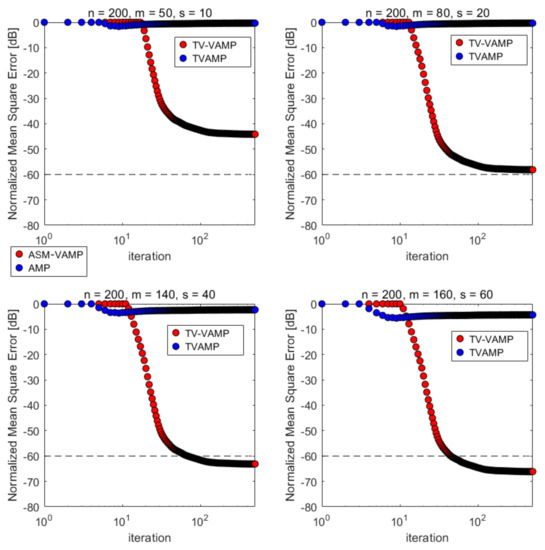
Figure 7. Normalized mean squared error (NMSE) convergence over iterations in the case of $k(\mathit{A})=500$ and $n=200$. Each curve is the average of 50 Monte Carlo samples.

Table 3. Average number of iterations to achieve NMSE = −60 dB for ill-conditioned measurements matrix.

Cases	$\mathit{s}=10,\mathit{m}=50$	$\mathit{s}=20,\mathit{m}=80$	$\mathit{s}=40,\mathit{m}=140$	$\mathit{s}=60,\mathit{m}=160$
TVAMP	∞	∞	∞	∞
TV-VAMP	∞	∞	60	43

4.4.2. Phase Transition

As before, we investigate the phase transition of TV-VAMP algorithm when the measurements matrix $\mathit{A}$ has an ill-conditioned number. Similarly, the empirical phase transition is calculated by CVX [42], and the experiment settings are the same as Section 4.2.2. Figure 8 confirms that the phase transition curve of TV-VAMP algorithm is still relatively accurate. In addition, it can be seen from the phase transition diagram in Figure 8 that when the gradient sparsity of the signal $s=[10,20]$, at least the number of measurements times $m=[72,89]$ is required to recover the original signal ($NMSE$ = −60 dB), while the number of measurements in the experiment is less than that. This is the reason why the NMSE of the TV-VAMP algorithm cannot converge in the first two cases in Table 3. Notably, the above is the purpose of our study of phase transition. We can determine the minimum number of observations at which the original signal can be reconstructed according to the phase transition curve, which is of great significance in practical applications.

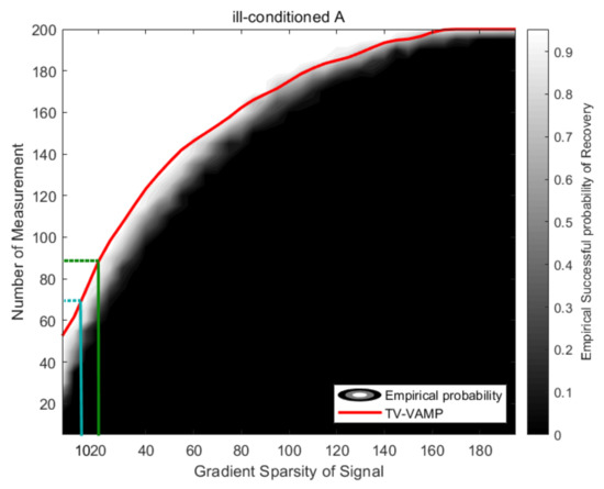
Figure 8. The figure shows phase transitions of CVX and TV-VAMP algorithm in the case of $k(\mathit{A})=500$ and $n=200$.

In the process of signal recovery, the measurement matrix plays an important role. The above numerical experiments show that the proposed TV-VAMP algorithm can be applied to a wider range of measurement matrices, especially when the measurement matrix is ill-conditioned, as it can still accurately recover the original signal, which verifies that our algorithm is robust to the measurement matrix.

5. Conclusions and Future Work

In this paper, we design a new iterative algorithm, called total variation vector approximate message passing (TV-VAMP), to solve total variation regularization problems and estimate the phase transitions of these problems. According to numerical simulations, we verify that the proposed algorithm is more robust than the TVAMP algorithm [32]. Specifically, our algorithm is suitable for a wider range of measurements distributions, including non-zero-mean Gaussian distribution measurements matrix and ill-conditioned measurements matrix. Furthermore, the experimental results confirm that our algorithm can better fit the empirical phase transition. Particularly, we can determine the minimum number of observations at which the real signal can be precisely recovered, which is meaningful in practical application; however, there is still a gap between the phase transition curve obtained by our algorithm and the empirical phase transition. The existence of the gap is caused by approximation steps in the derivation of TV-VAMP algorithm.

We believe that the gap could be improved if we can optimize the approximation steps in this paper. To be specific, we are going to find a more appropriate approximation to the mean and average variance of the distribution $b_{sp}\left(\mathit{z}\right)$ in Equation (23). Apart from that, it is necessary to note that, according to the existing references [29,30], state evolution can accurately predict the phase transition of the corresponding model, which is a simple scalar iterative scheme that can track dynamics of approximate message passing algorithm. Therefore, we prepare to deduce the state evolution of the total variation model and further infer the corresponding optimal TV-VAMP algorithm on the basis of state evolution.

References

- Donoho, D.L. Compressed sensing. IEEE Trans. Inf. Theory 2006, 52, 1289–1306. [Google Scholar] [CrossRef]
- Candès, E.J.; Romberg, J.; Tao, T. Robust uncertainty principles: Exact signal reconstruction from highly incomplete frequency information. IEEE Trans. Inf. Theory 2006, 52, 489–509. [Google Scholar] [CrossRef]
- Eldar, Y.C.; Kutyniok, G. Compressed Sensing: Theory and Applications; Cambridge University Press: Cambridge, UK, 2012. [Google Scholar]
- Rudin, L.I.; Osher, S.; Fatemi, E. Nonlinear total variation based noise removal algorithms. Phys. D 1992, 60, 259–268. [Google Scholar] [CrossRef]
- Wu, Q.; Li, Y.; Lin, Y. The application of nonlocal total variation in image denoising for mobile transmission. Multimed. Tools Appl. 2017, 76, 17179–17191. [Google Scholar] [CrossRef]
- Hosseini, M.S.; Plataniotis, K.N. High-accuracy total variation with application to compressed video sensing. IEEE Trans. Image Process. 2014, 23, 3869–3884. [Google Scholar] [CrossRef] [PubMed]
- Chan, T.; Esedoglu, S.; Park, F.; Yip, A. Total variation image restoration: Overview and recent developments. In Handbook of Mathematical Models in Computer Vision; Springer: Berlin/Heidelberg, Germany, 2006; pp. 17–31. [Google Scholar]
- Chan, T.; Marquina, A.; Mulet, P. High-order total variation-based image restoration. SIAM J. Sci. Comput. 2000, 22, 503–516. [Google Scholar] [CrossRef]
- Bredies, K.; Kunisch, K.; Pock, T. Total generalized variation. SIAM J. Imaging Sci. 2010, 3, 492–526. [Google Scholar] [CrossRef]
- Benning, M.; Brune, C.; Burger, M.; Müller, J. Higher-order TV methods—Enhancement via Bregman iteration. J. Sci. Comput. 2013, 54, 269–310. [Google Scholar] [CrossRef]
- Afonso, M.V.; Bioucas-Dias, J.M.; Figueiredo, M.A. An augmented Lagrangian approach to the constrained optimization formulation of imaging inverse problems. IEEE Trans. Image Process. 2010, 20, 681–695. [Google Scholar] [CrossRef]
- Figueiredo, M.A.; Bioucas-Dias, J.M. Restoration of Poissonian images using alternating direction optimization. IEEE Trans. Image Process. 2010, 19, 3133–3145. [Google Scholar] [CrossRef]
- Almeida, M.S.; Figueiredo, M. Deconvolving images with unknown boundaries using the alternating direction method of multipliers. IEEE Trans. Image Process. 2013, 22, 3074–3086. [Google Scholar] [CrossRef]
- Matakos, A.; Ramani, S.; Fessler, J.A. Accelerated edge-preserving image restoration without boundary artifacts. IEEE Trans. Image Process. 2013, 22, 2019–2029. [Google Scholar] [CrossRef]
- Kabanava, M.; Rauhut, H. Analysis ℓ1-recovery with Frames and Gaussian Measurements. Acta. Appl. Math. 2015, 140, 173–195. [Google Scholar] [CrossRef]
- Daei, S.; Haddadi, F.; Amini, A. Living Near the Edge: A Lower-Bound on the Phase Transition of Total Variation Minimization. IEEE Trans. Inf. Theory 2020, 66, 3261–3267. [Google Scholar] [CrossRef]
- Genzel, M.; Kutyniok, G.; März, M. ℓ1-Analysis minimization and generalized (co-)sparsity: When does recovery succeed? Appl. Comput. Harmon. Anal. 2021, 52, 82–140. [Google Scholar] [CrossRef]
- Chandrasekaran, V.; Sanghavi, S.; Parrilo, P.A.; Willsky, A.S. Rank-sparsity incoherence for matrix decomposition. SIAM J. Optim. 2011, 21, 572–596. [Google Scholar] [CrossRef]
- Donoho, D.L.; Gavish, M.; Montanari, A. The phase transition of matrix recovery from Gaussian measurements matches the minimax MSE of matrix denoising. Proc. Natl. Acad. Sci. USA 2013, 110, 8405–8410. [Google Scholar] [CrossRef]
- Donoho, D.; Tanner, J. Observed universality of phase transitions in high-dimensional geometry, with implications for modern data analysis and signal processing. Philos. Trans. R. Soc. A 2009, 367, 4273–4293. [Google Scholar] [CrossRef]
- Candès, E.J.; Eldar, Y.C.; Needell, D.; Randall, P. Compressed sensing with coherent and redundant dictionaries. Appl. Comput. Harmon. Anal. 2011, 31, 59–73. [Google Scholar] [CrossRef]
- Rudelson, M.; Vershynin, R. On sparse reconstruction from Fourier and Gaussian measurements. Comm. Pure Appl. Math. 2008, 61, 1025–1045. [Google Scholar] [CrossRef]
- Stojnic, M. Various thresholds for ℓ1-optimization in compressed sensing. arXiv 2009, arXiv:0907.3666. [Google Scholar]
- Chandrasekaran, V.; Recht, B.; Parrilo, P.A.; Willsky, A.S. The Convex Geometry of Linear Inverse Problems. Found. Comput. Math. 2012, 12, 805–849. [Google Scholar] [CrossRef]
- Amelunxen, D.; Lotz, M.; McCoy, M.B.; Tropp, J.A. Living on the edge: Phase transitions in convex programs with random data. Inf. Inference J. IMA 2014, 3, 224–294. [Google Scholar] [CrossRef]
- Kabanava, M.; Rauhut, H.; Zhang, H. Robust analysis ℓ1-recovery from Gaussian measurements and total variation minimization. Eur. J. Appl. Math. 2014, 26, 917–929. [Google Scholar] [CrossRef]
- Daei, S.; Haddadi, F.; Amini, A. Sample Complexity of Total Variation Minimization. IEEE Signal Process. Lett. 2018, 25, 1151–1155. [Google Scholar] [CrossRef]
- Feng, O.Y.; Venkataramanan, R.; Rush, C.; Samworth, R.J. A unifying tutorial on Approximate Message Passing. Found. Trends Mach. Learn. 2022, 15, 335–536. [Google Scholar] [CrossRef]
- Donoho, D.L.; Maleki, A.; Montanari, A. Message passing algorithms for compressed sensing. Proc. Nat. Acad. Sci. USA 2009, 106, 18914–18919. [Google Scholar] [CrossRef]
- Bayati, M.; Montanari, A. The Dynamics of Message Passing on Dense Graphs, with Applications to Compressed Sensing. IEEE Trans. Inf. Theory 2011, 57, 764–785. [Google Scholar] [CrossRef]
- Ma, Y.; Rush, C.; Baron, D. Analysis of Approximate Message Passing With Non-Separable Denoisers and Markov Random Field Priors. IEEE Trans. Inf. Theory 2019, 65, 7367–7389. [Google Scholar] [CrossRef]
- Donoho, D.L.; Johnstone, I.; Montanari, A. Accurate Prediction of Phase Transitions in Compressed Sensing via a Connection to Minimax Denoising. IEEE Trans. Inf. Theory 2013, 59, 3396–3433. [Google Scholar] [CrossRef]
- Liu, Y.; Mi, T.; Li, S. Compressed Sensing With General Frames via Optimal-Dual-Based ℓ1-Analysis. IEEE Trans. Inf. Theory 2012, 58, 4201–4214. [Google Scholar] [CrossRef]
- Nam, S.; Davies, M.; Elad, M.; Gribonval, R. The cosparse analysis model and algorithms. Appl. Comput. Harmon. Anal. 2013, 34, 30–56. [Google Scholar] [CrossRef]
- Kschischang, F.R.; Frey, B.J.; Loeliger, H.A. Factor graphs and the sum-product algorithm. IEEE Trans. Inf. Theory 2001, 47, 498–519. [Google Scholar] [CrossRef]
- Koller, D.; Friedman, N. Probabilistic Graphical Models: Principles and Techniques; MIT Press: Cambridge, MA, USA, 2009. [Google Scholar]
- Wainwright, M.J.; Jordan, M.I. Graphical models, exponential families, and variational inference. Found. Trends Mach. Learn. 2008, 1, 1–305. [Google Scholar] [CrossRef]
- Loeliger, H.A. An introduction to factor graphs. IEEE Signal Process. Mag. 2004, 21, 28–41. [Google Scholar] [CrossRef]
- Frey, B.J.; Kschischang, F.R.; Loeliger, H.A.; Wiberg, N. Factor graphs and algorithms. In Proceedings of the Annual Allerton Conference on Communication Control and Computing, Monticello, IL, USA, 1 October 1997; Volume 35, pp. 666–680. [Google Scholar]
- Rangan, S.; Schniter, P.; Fletcher, A.K. Vector Approximate Message Passing. IEEE Trans. Inf. Theory 2019, 65, 6664–6684. [Google Scholar] [CrossRef]
- Gelman, A.; Carlin, J.B.; Stern, H.S.; Rubin, D.B. Bayesian Data Analysis; Chapman and Hall/CRC: Boca Raton, FL, USA, 1995. [Google Scholar]
- Grant, M.; Boyd, S. CVX: Matlab Software for Disciplined Convex Programming, Version 2.1. 2014. Available online: https://web.stanford.edu/~boyd/papers/pdf/disc_cvx_prog.pdf (accessed on 12 August 2022).
Publisher’s Note: MDPI stays neutral with regard to jurisdictional claims in published maps and institutional affiliations. |
© 2022 by the authors. Licensee MDPI, Basel, Switzerland. This article is an open access article distributed under the terms and conditions of the Creative Commons Attribution (CC BY) license (https://creativecommons.org/licenses/by/4.0/).