Geo-Location Method for Images of Damaged Roads

Abstract

Due to the large difference between normal conditions and damaged road images, geo-location in damaged areas often fails due to occlusion or damage to buildings and iconic signage in the image. In order to study the influence of post-war building and landmark damage conditions on the geolocation results of localization algorithms, and to improve the geolocation effect of such algorithms under damaged conditions, this paper used informative reference images and key point selection. Aiming at the negative effects of occlusion and landmark building damage in the retrieval process, a retrieval method called reliability- and repeatability-based deep learning feature points is proposed. In order to verify the effectiveness of the above algorithm, this paper constructed a data set consisting of urban, rural and technological parks and other road segments as a training set to generate a database. It consists of 11,896 reference images. Considering the cost of damaged landmarks, an artificially generated method is used to construct images of damaged landmarks with different damage ratios as a test set. Experiments show that the database optimization method can effectively compress the storage capacity of the feature index and can also speed up the positioning speed without affecting the accuracy rate. The proposed image retrieval method optimizes feature points and feature indices to make them reliable against damaged terrain and images. The improved algorithm improved the accuracy of geo-location for damaged roads, and the method based on deep learning has a higher effect on the geo-location of damaged roads than the traditional algorithm. Furthermore, we fully demonstrated the effectiveness of our proposed method by constructing a multi-segment road image dataset.

1. Introduction

The Global Navigation Satellite System (GNSS) has been a relatively mature posi-tioning technology, and it has been widely used in many fields. In the actual use of the GNSS positioning method, the ground signal strength is weak, and the civil coding structure is open, which makes the GNSS signal vulnerable to interference under complex electromagnetic interference and is prone to positioning failure when it is interfered by malicious deception. Although nowadays, smart devices have the function of obtaining geographic tags, when the GNSS signal is interfered and still needs to be positioned, users cannot rely on GNSS to obtain positioning information, and they are located in cities, post-disaster damaged areas, and geodetic control points. Being damaged and unable to be used normally, the inertial navigation equipment cannot be effectively calibrated, so it is difficult to use the inertial navigation equipment for precise positioning. In recent years, visual place recognition has received great attention in the field of machine vision, which can be used to solve the problem of location information localization. If relatively accurate geo-location information is added to these images, they can be of great benefit in areas such as outdoor localization [1], pedestrian detection [2], autonomous driving [3], etc. In addition, pictures with geolocation information can also help environment perception technology for robots [4] and urban construction. Therefore, it is a problem that needs to be researched to identify the visual position of damaged road images under the condition of interference with GNSS signals, and to perform geolocation at the same time.

In order to correctly localize a road image, the image-based localization (IBL) task matches image features with unknown location information to image feature labels with GNSS information in the database [5]. Precise image geo-location has long been a challenge, and geolocation using images involves image retrieval, including identifying, extracting, and indexing geographic information features from massive databases. Simultaneous localization and mapping (SLAM) is also widely used in image geolocation to map and locate objects. However, under the condition of interference of GNSS signals, such as damaged landmarks, traditional image retrieval methods cannot capture enough features, resulting in retrieval failure, and the matching results of SLAM will also be affected. It is impossible to draw maps and calculate latitude and longitude under conditions where landmark features in the image are corrupted, or where the image is obscured or contaminated. Additionally, different types of features will be highlighted under different conditions [6]. Under extreme conditions such as occlusion and landmark damage, the altered landform hides most of the features, making visual location recognition difficult. In the future network system, it is also a very important requirement for the unification of location information in the same coordinate system with high accuracy. The traditional method of map-based emergency positioning has gradually been difficult to meet the requirements of high precision.

Content-based image retrieval (CBIR) is one of the important applications of deep learning in computer vision. The purpose of CBIR is to search images with similar content from the database. Under the condition that the landmarks in the image are damaged, the change of the scene in the image will increase the difficulty of image retrieval, and the feature points used for positioning in the image will change. Deep learning has been successful in many fields in recent years, including computer vision (CV) [7,8,9,10].

The descriptors of the whole image are calculated directly using the global descriptor method. The Gist descriptor proposed by Olive [11] et al. is a widely used global feature descriptor, which uses Gabor filters to extract image information in different directions and frequencies and compress them into vectors as image descriptions. Lowry et al. [12] used online learning to train PCA transformation and pointed out that the PCA features corresponding to the first half of the dimension represent similar information in continuous image sequences and are susceptible to environmental changes, while the second half has environmental conditions invariance and can better correspond to the environment variety. Ulrich et al. [13] used panoramic color image histograms combined with nearest neighbors to learn to match images. Local feature point descriptors can also generate global image descriptions. For example, Sunderhauf et al. [14] first down-sample the image and then calculate the brief descriptor around the center of the down-sampled image, which is suitable for some large-scale applications.

Local features are generally more robust to occlusion, scale, rotation, and illumination changes. These methods start with a detection phase, where points of interest are found in the image, followed by a description phase, where a bit of metric is extracted from around these key points. Local features have better recognition capability, thus improving the recognition rate and reducing the detection error. The most commonly used one is the SIFT algorithm proposed by Lowe [15], which uses a Gaussian convolution kernel to construct a scale space and extracts feature points in an image pyramid, where the descriptor of each feature point consists of a 128-dimensional vector. The algorithm is invariant to scale, rotation, and illumination, making it widely used in early visual localization [16,17,18], but because the SIFT algorithm is very time-consuming to extract feature points and descriptors, the subsequent development of algorithms such as the SURF algorithm proposed by Bay et al. [19] and the ORB algorithm proposed by Rubbee et al. [20] mostly improve efficiency at the expense of performance.

The complementary advantages of local feature descriptors and global feature descriptors have led many researchers to use global description methods to generate descriptors for local regions of images. Gradually, many object feature extraction methods have emerged, such as the RPN [21] network and the edge-boxes algorithm [22]. The RPN obtains the potential area of a specific target through the learning method, and the edge-boxes algorithm judges whether it contains an object by the size of the outline information inside the box, which is universal. The method of generating local regions from the original image and then generating global descriptors for the local regions takes into account appearance invariance and perspective invariance and makes the scene definition more flexible [23]. A large amount of literature [24,25,26,27] has shown that deep learning-based feature extraction methods outperform traditional methods, especially deep convolutional neural network (DCNN)-based feature extraction methods for image retrieval and feature point extraction by deep learning-based features for location identification, which can achieve results unattainable by traditional algorithms.

Accurate geo-localization has long been a challenge [28], especially under obscured content in images, and there are still many problems to be solved. First, errors in position recognition can cause the wrong positioning of the positioning algorithm, thus reducing the positioning accuracy and even leading to ultimate positioning failure. Secondly, most of the existing visual location recognition algorithms are content-based. However, typical landmarks and building features on the same road are easily altered by damage from various factors, resulting in a large change in the content of the image even in the same place.

According to the image representation method, a reasonable decision model is used to infer the final recognition point, and the decision model can effectively improve the accuracy and recall rate of location recognition. The matching of input images to stored database images treats the recognition problem as a large-scale retrieval problem. There are many solutions around the problem of how to retrieve images quickly and accurately, such as bag-of-words (BoW) [29] and its derivatives. The core of this series of methods is to encode images into dictionaries with reference to the idea of text search. Search and match in the form of a dictionary. This derivative method also appears to be more effective. For example, Cummins [30] et al. combined BoW with concepts to search and match images and achieved very good results. In addition, FAB-MAP2.0 [31] uses an inverse index structure to store map description information. The images that own the term are stored under each term, not under each image, making the search space size only related to the number of terms and not limited by the map size. It is evident from the related works that most researchers have tried to eliminate the effects of extreme conditions using various techniques.

Aiming at the problem of damaged image geolocation, this paper proposes a road image geolocation method for damaged buildings and landmark areas. The method employs a three-step strategy.

• For data with low occlusion or useful information, we used improved semantic segmentation algorithms to filter the dataset and reduce the number of images in the dataset to speed up localization time;
• Aiming at the phenomenon that the image damage area interferes with the image retrieval results, to perform coarse geo-location, we propose a deep learning feature point-based image retrieval method;
• Fine-grained geo-location using heading angle information was finally completed with experimental validation on our dataset, proving the effectiveness of our method.

The remainder of this paper is organized as follows. Section 2 introduces the implementation of the method and expounds its rationale. Section 3 constructs the database using our self-harvested data as the training set and the generated damaged road images as the test set and describes the experimental procedure and results in detail. Section 4 lists the conclusions and future work.

2. Methods

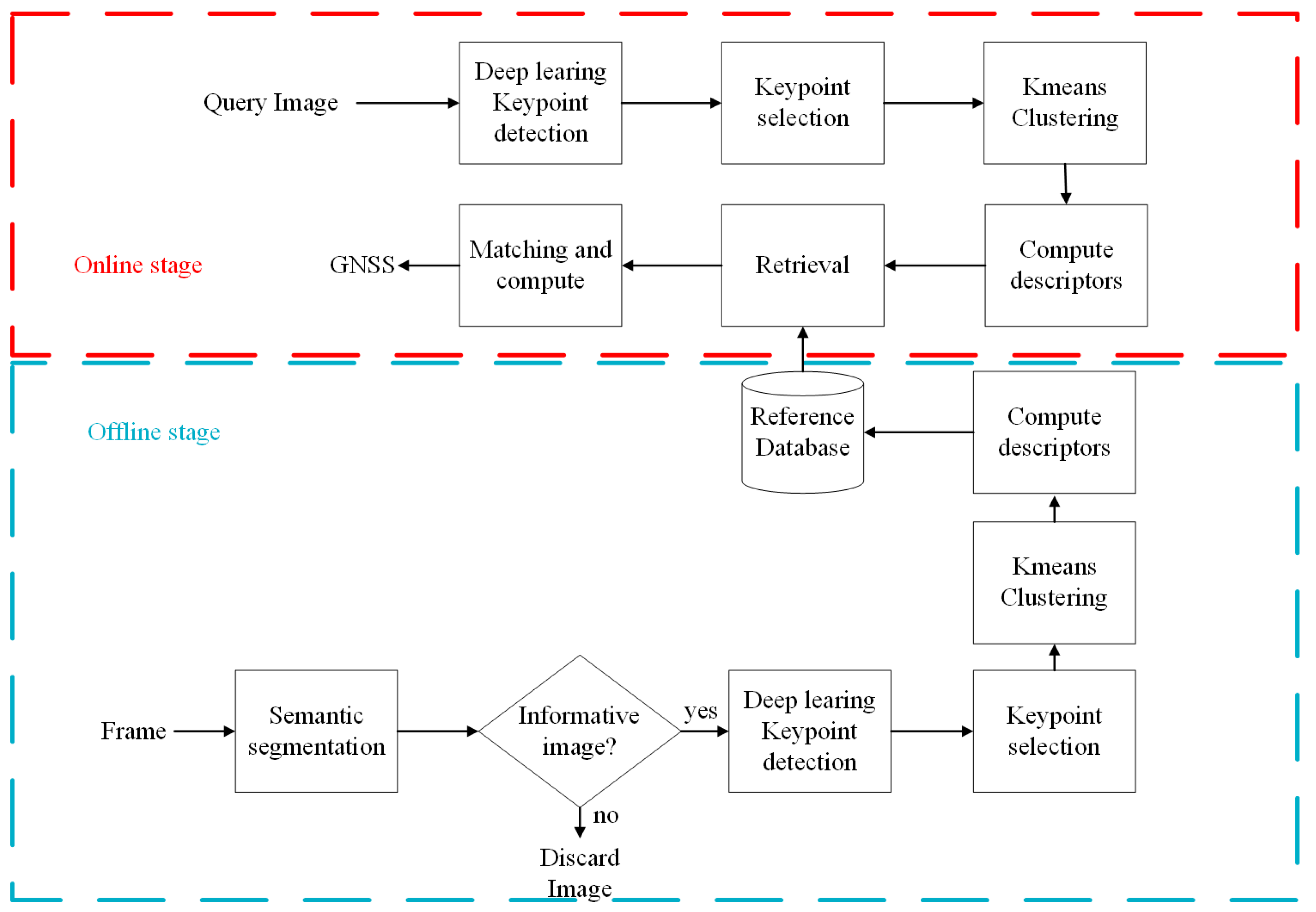
Although previous methods have also provided relatively accurate geographic location information, the proposed method provided the ability to maintain accurate geographic location information under the condition of environmental damage to road images. This is achieved through the design of reference dataset optimization and retrieval algorithms. The database optimization is performed by an improved semantic segmentation algorithm that automatically filters the information in it in batch. The proposed system consists of two key parts: an online part and an offline part, as shown in Figure 1. In the user’s daily work, the system is used to collect data of typical features that may be applied in urban, desert and Gobi environmental areas. After data training processing, a corresponding relationship can be established through the time information and the location information obtained by applying the multi-source navigation and positioning data fusion method to form a data pair and store it in the offline feature database. When the user cannot quickly obtain accurate positioning during emergency positioning, the online system can respond quickly and obtain high-precision positioning information. When the location is around the objects stored in the offline database. It can use the stereo data binocular vision fast matching method to calculate and match the similarity between the real-time captured image and the database image. At the same time, the spatial position information of the typical feature is read, and the relative position relationship between the database image shooting point and the online point to be measured is established according to the rotation matching matrix obtained by the visual method to transmit the position information, and finally, the positioning information is obtained.

2.1. Dataset Filtering and Damaged Territory Dataset Construction Based on Improved Semantic Segmentation Methods

2.1.1. Improved Semantic Segmentation Algorithm

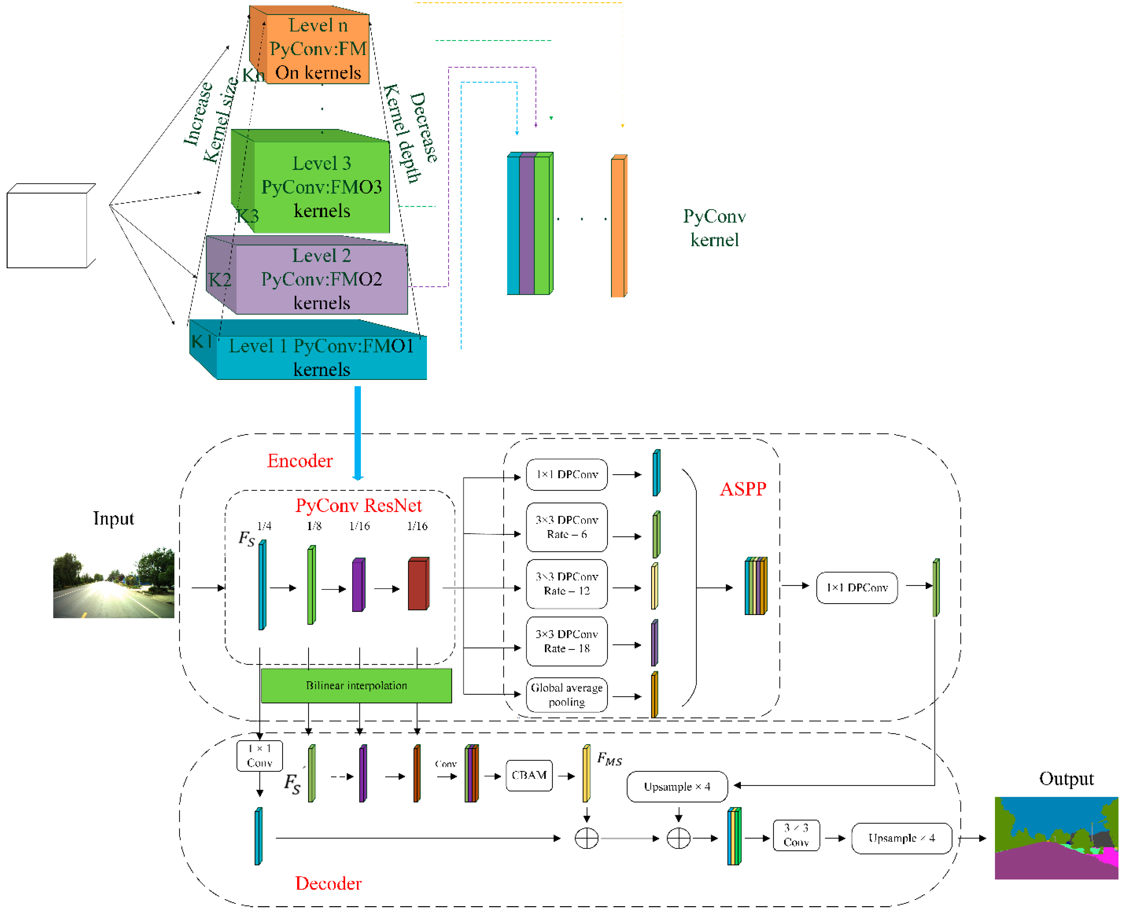
For the current Deeplab v3+ [32] semantic segmentation algorithm that does not use high-resolution shallow features, the phenomenon of wrong segmentation and omission of segmentation occurs. This paper uses the improved semantic segmentation algorithm proposed by the author [33]. The improved Deeplab v3+ network structure is shown in Figure 2. Compared with the original Deeplab v3+ algorithm, the main structure is still the encoder–decoder structure, and the backbone network used in the original algorithm is ResNet [34]. The purpose of the improved network is to improve the “loss” of information in the semantic segmentation task for damaged buildings and damaged road signs in damaged road images. The purpose of the improved algorithm is to segment the edge information of the damaged object more accurately and accurately and to improve or prevent this phenomenon of wrong segmentation and missing segmentation.

The main improvements are as follows:

• In the coding layer, the backbone network is improved, and PyConv [35] is introduced. The main idea of introducing PyConv is to divide the input features into different groups for pyramid convolution and perform convolution calculations independently. Compared with standard convolution, PyConv can enlarge the receptive field of the kernel without increasing the computational cost. It can also apply different types of kernels in parallel to process the input, with different spatial resolutions and depths. Along the Resnet network, we can identify four main stages based on the spatial size of the feature maps. The pyramid convolution kernel divides the output channels into four groups in the first stage of the network, each group uses the convolution kernel size of 3 × 3, 5 × 5, 7 × 7, 9 × 9, and the number of output channels is 64, 64, 64, 64. The corresponding grouped convolution group numbers are 1, 4, 8, and 16, respectively. The second stage divides the output channels into three groups, and each group uses convolution kernel sizes of 3 × 3, 5 × 5, and 7 × 7, respectively. The number of output channels is 128, 128, 256, respectively. The corresponding grouped convolution group numbers are 1, 4, and 8, respectively. The third stage divides the output channels into two groups. The size of the convolution kernels used in each group is 3 × 3 and 5 × 5, respectively, and the number of output channels is 512 and 512, respectively. The corresponding grouped convolution group numbers are 1 and 4, respectively. The fourth stage convolves all channels with a 3 × 3 convolution kernel, and the number of groups is 1. The specific parameter details of pyconv are shown in

  Table 1. Parameter table of each layer of pyconv.

  Layers	Pyconv Kernels	Pyconv Kernel Output Chanels	Pyconv_Groups
  Layer1	(3,5,7,9)	(64,64,64,64)	(1,4,8,16)
  Layer2	(3,5,7)	(128,128,256)	(1,4,8)
  Layer3	(3,5)	(512,512)	(1,4)
  Layer4	(3)	(2048)	(1)

  .
• Replace the normal convolution in atrous spatial pyramid pooling (ASPP) with depth-wise separable convolution. That is, all 3 × 3 convolutional layers are changed to 3 × 3 depth-wise separable convolutions, reducing the parameters of the network layer and speeding up the training efficiency with little impact on the running results.
• In the decoding layer, the original algorithm is improved mainly by combining the outputs of different stages of the backbone residual network. Since the feature maps generated by each layer of the backbone network are critical to the final segmentation map, while the original segmentation network Deeplab v3+ uses only the high-resolution features of the first layer, i.e., it uses a quarter-sized feature map. In this paper, the feature maps output by the second and third layers are used. The size of the feature maps is 1/8, 1/16 and 1/16, respectively, and the number of channels is 512, 1024 and 2048, respectively. The output of each feature layer is upsampled by a bilinear interpolation operation, and the number of channels is reduced to 64 by 1 × 1 convolution. The output three feature maps are channel superimposed into a feature map of 1/4 size and 128 channels, which is passed through the attention mechanism module CBAM [36]. This makes it easier for the network to focus on the key locations where features are extracted and increases the network’s ability to extract edge features. The feature map processed by attention mechanism is superimposed with shallow features and deep features after quadruple up-sampling, the number of channels is adjusted to 256 by 3 × 3 convolution, and finally, the feature map is restored to the original image size by upsampling, and the feature map is divided into pre-defined categories by the classifier and output.

This approach helps to encode both global and local environments due to the use of features learned at multiple scales to enrich the representation of shallow features. In this paper, we borrow the idea of multi-scale self-guided attention network design for medical image segmentation proposed by Sinha et al. [37]. A new combinatorial network of multi-scale attention mechanisms is proposed, which is embedded in the decoding layer of the original Deeplab v3+ through the attention mechanism CBAM after the combination. Specifically, in our setting, features at multiple scales are denoted as $F_S$, where S represents the number of layers where the feature map is located. Since the features of each layer have different resolutions, they are upsampled to the same resolution by bilinear interpolation, so that the output amplified feature map is denoted as $F_S^{\prime }$ and the corresponding S denotes the number of layers corresponding to the feature map. Then, without changing the original network structure, $F_1$ is output by 1 × 1 convolution, the subsequent $F_2^{\prime }$, $F_3^{\prime }$, and $F_4^{\prime }$ are connected to form a tensor (tensor), a multi-scale feature map is obtained by convolution, and then the output multi-scale feature map is passed through the CBAM module to obtain $F_{MS}$, where $F_{MS}$ is shown in Equation (1):

$$F_{MS}=CBAM(Conv(F_2^{\prime }+F_3^{\prime }+F_4^{\prime }))$$

(1)

2.1.2. Database Optimization

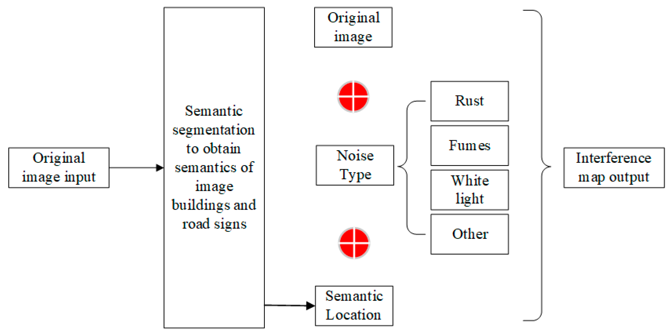
Using an improved semantic segmentation algorithm based on deep learning can segment semantic information from images and identify what different regions of the image represent. Buildings and road signs play an indispensable role in road image matching and localization. Relatively speaking, static and dynamic objects in complex scenes of road images, such as pedestrians, vehicles, trees, etc., contribute unstable or even almost meaningless to the matching and recognition effects of road images. The semantic segmentation approach is proposed to address this problem, and in this paper, its main contribution is to identify the effective feature regions in the image and to identify the portion of buildings and road signs in the image.

The filtering of the data is achieved by removing privacy-infringing, duplicate and unfocused images from the data through semantic segmentation and eliminating images where buildings and road signs make up too small a proportion of the images before the dataset is built. The specific method is as follows. The images are fed into the network for segmentation process to obtain the classification matrix of the images. The number of pixel points belonging to buildings and landmarks in the image is counted and compared with a fixed threshold. The comparison result is used to determine whether the image should be sieved or not. For a 2048 × 1080 image, the pixel threshold is 10,000 for buildings and 5000 for landmarks, and when the number of corresponding pixel points is less than the threshold, it is determined that the image has less content, and the image is excluded. Otherwise, it will be kept.

2.1.3. Destruction Area Dataset Construction

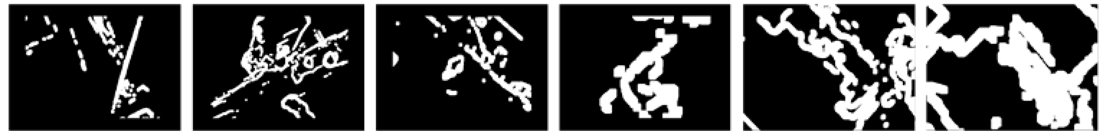
The damaged road condition studied in this paper refers to the road environment under various regional conditions. Landmarks are difficult to identify in images due to thick smoke, fog, or rust, later man-made damage to road signs and buildings on both sides of the road. Many of these regional conditions include highway sections, urban roads, and rural sections. In this case, ordinary image search and localization algorithms will face great challenges. In order to simulate the above-mentioned damaged area conditions under realistic conditions, this paper uses partial masks from the irregular mask dataset proposed in the paper by Nvidia [38] to constitute the damage condition dataset. The irregular mask dataset is generated by collecting random streaks and masks of arbitrarily shaped holes, the source of which is described in [39], using occlusion or de-occlusion mask estimation methods between two consecutive frames of the video result. This dataset has a total of six masks with different hole-to-area ratios of (0.01,0.1], (0.1,0.2], (0.2,0.3], (0.3,0.4], (0.4,0.5], and (0.5,0.6]. The mask images used in this paper are 48 images from these six classes of masks with different hole-to-area ratios selected randomly, with eight images selected from each class. The selected mask masks are distributed in the center and all around the periphery of the images, some of which are shown in Figure 3.

The damage condition dataset consists of the above irregular mask dataset, four kinds of mask maps simulating various masking factors in real environment and original images, where the mask maps include corrosion, light smoke, rust and smoke, etc. These mask maps are created by Photoshop software and saved in picture form by means of layers. The mask maps used in this paper are shown in Figure 4.

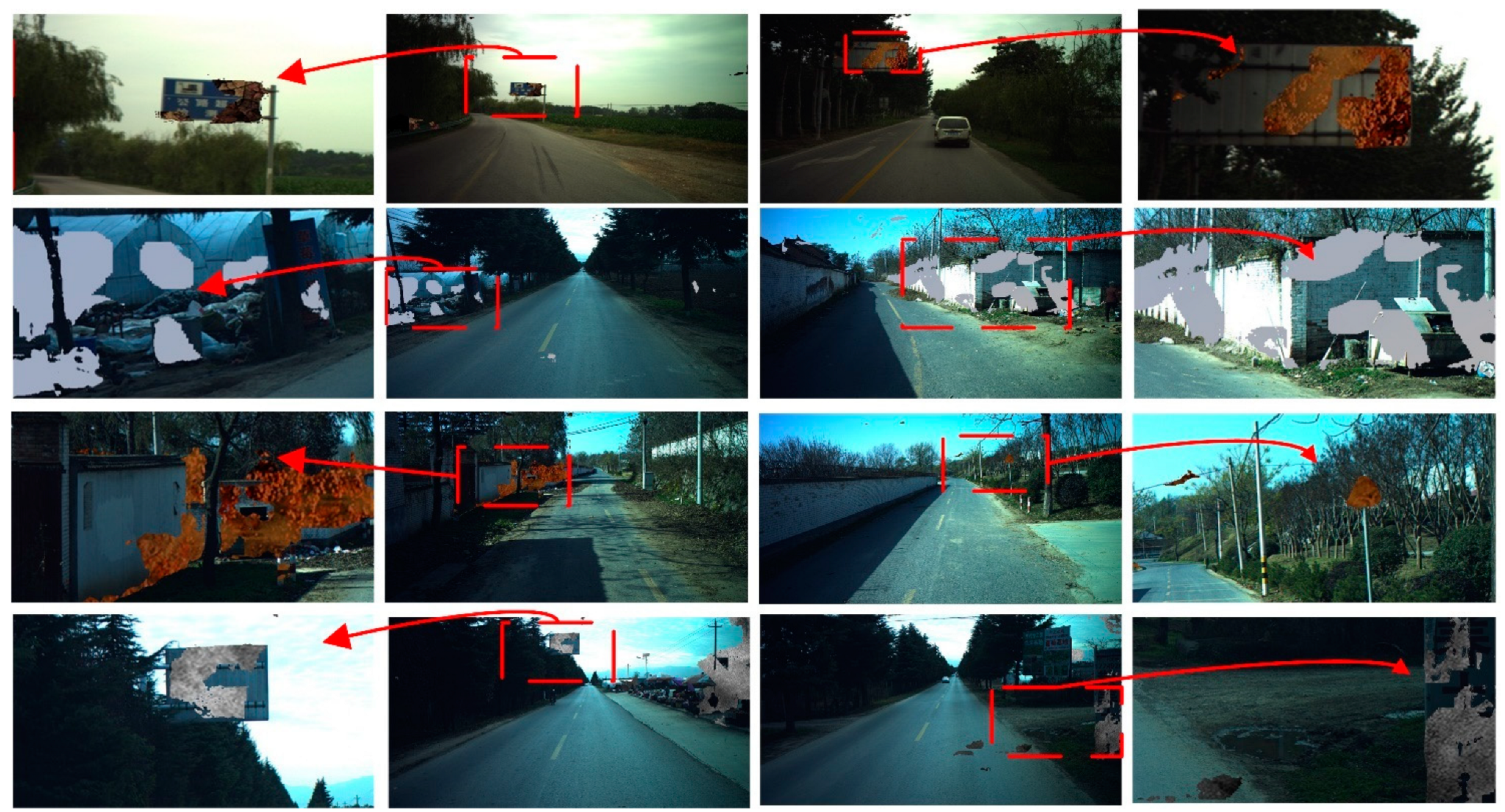
On the basis of the collected data set of a certain road section, it is damaged and processed. Road signs and buildings in the image are first identified using an improved semantic segmentation algorithm. These two types of information are not easily disturbed by seasonal and illumination factors, so they can be considered as valid information. The randomly generated “damage pollution” is used to cover the image, and the damage ratio of each group is calculated according to the area ratio of the occluded road signs and buildings to the whole image. Generate the damage image data set. The process of damage masking on the original image is shown in Figure 5. The part of the generated damaged geographical condition dataset is shown in Figure 6.

2.2. Coarse Geo-Location Based on Image Retrieval

In order to perform accurate geolocation calculations, coarse geolocation based on image retrieval is performed first in the online phase after optimizing the dataset using an improved semantic segmentation algorithm. The purpose of coarse localization by image retrieval is to find the best match for the query image.

In this paragraph, we will describe the process of image retrieval using our method. This includes using deep learning feature points for image retrieval. First, we input the images into the neural network. Reliable and repeatable feature points and descriptors are extracted by this algorithm. The feature point and descriptor extraction method used in this paper refers to the feature point detection method proposed by Jerome Revaud [40] et al. in 2019. 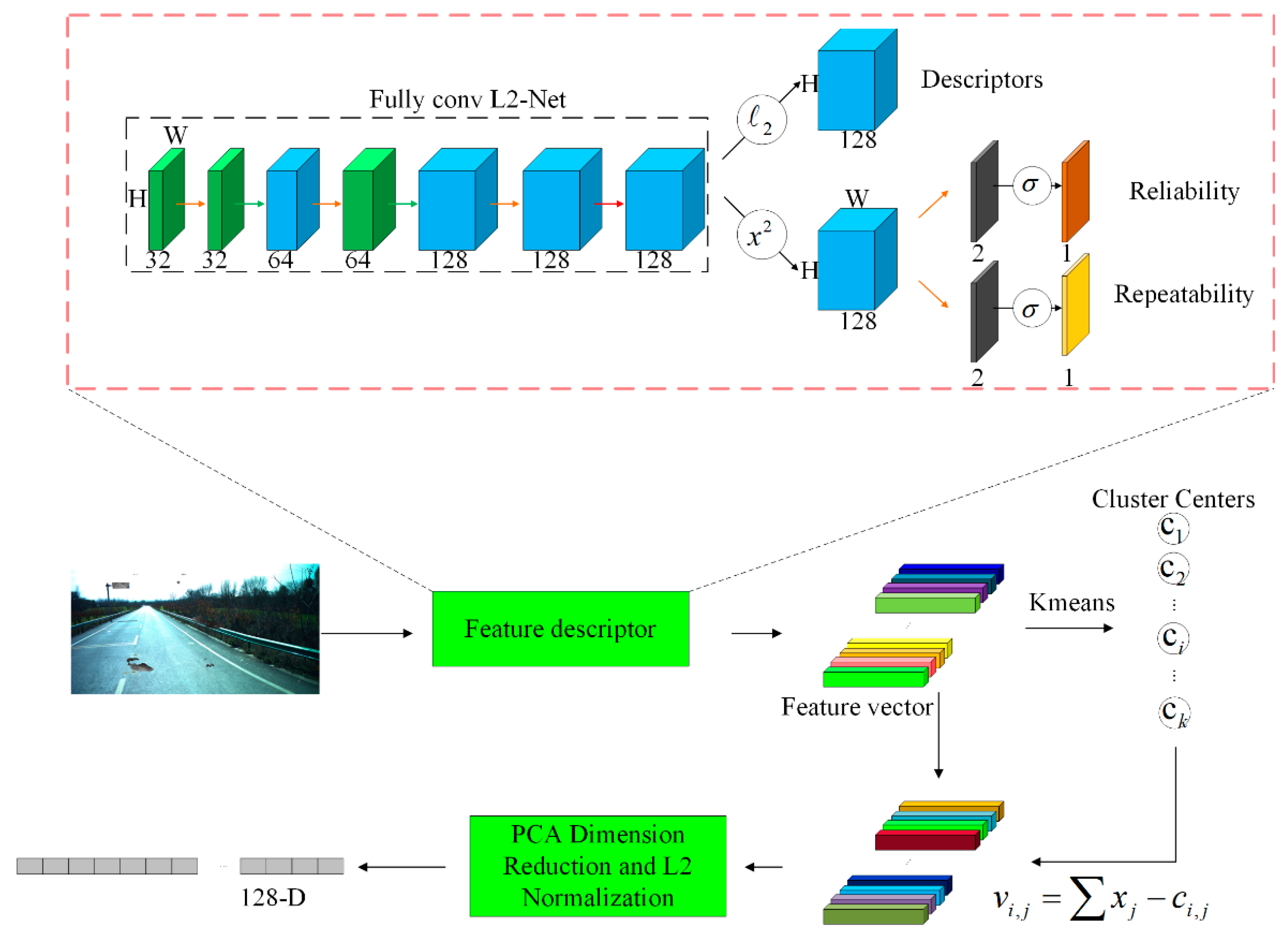The introduced model is shown in Figure 7. Among them, repeatable feature points can still be detected in various shooting angles, light, and seasonal changes, and reliable ones can make the descriptors match correctly. This feature point extraction method believes that descriptors should be learned only in regions with high confidence because good keypoints should not only be repeatable, but also discriminative. Therefore, in the learning process, the detection and description processes are seamlessly combined to learn, thereby improving the reliability of the descriptor because the damaged road image content targeted in this paper is subject to external interference and occlusion. Using content-based retrieval methods will reduce the retrieval accuracy in the cases addressed in this paper. Using this feature point detection method can adapt to the situation that the image content is changed due to damage and man-made damage under the damaged condition, and the damaged road section can also be considered as the situation where the content in the image is occluded. Using the introduced method can extract more reliable and effective feature points and descriptors in this case. Damaged images can be expressed more effectively. After that, the clustering method can be used to train the codebook, the features of each image can be accumulated with the nearest cluster center to obtain a feature matrix, and then a feature vector can be created from the matrix. Finally, the PCA dimension reduction and normalization operations are performed on the accumulated descriptors.

The feature extraction process in image retrieval is shown in Figure 7. The specific process is as follows.

• Reliable and repeatable feature points and descriptors are extracted using a feature point extraction network. These descriptors are later clustered using the KMeans algorithm and the training codebook;
• The features of each image are accumulated with the nearest cluster center;
• PCA dimension reduction is performed on the accumulated feature vectors, and they are normalized;
• A shortlist of the top-matched images is generated based on the feature vector;
• The images in the shortlist are re-ranked by local descriptor matching using the Hamming distance and by checking the geometrical consistency using the distance ratio coherence.

The backbone network is L2-Net [41], and two modifications have been made. The first is to use extended convolution to replace the original down-sampling at the down-sampling place, so that the original resolution of the feature map is maintained at each stage. The second is to replace the final 8 × 8 convolution with three 2 × 2 convolutions.

The output of the backbone network is a 128-dimensional feature map, followed by three outputs. (1) The descriptor X of each pixel is obtained by L2 normalization; (2) S is obtained by a square operation, 1 × 1 convolution, and softmax; (3) R is obtained by the same operation as (2).

The three outputs of this network are as follows.

• $X\in {ℝ}^{H\times W\times D}$ corresponds to the descriptor;
• $S\in {[0,1]}^{H\times W}$ corresponds to feature descriptor location (repetitiveness);
• $R\in {[0,1]}^{H\times W}$ corresponds to descriptor reliability.

The network outputs dense local descriptors and two associated repeatability and reliability confidence maps. One of them estimates keypoints to be repeatable, and the other estimates that their descriptors are separable. Finally, keypoints are taken from where the response is maximized for these two graphs.

2.3. Fine-Grained Geographic Alignment Implementation Based on Feature Matching

Our method usually uses the same camera with two images taken at two locations. Let the coordinates of the space point P in the world coordinate system be P. Because the world coordinate system and the camera coordinate system of the left view overlap, the coordinates are also P in the left camera coordinate system and RP + t in the right view camera coordinate system.

R and T are calculated from the essential matrix and fundamental matrix. The calculation method is shown in Equations (2) and (3).

$$E=t^{\wedge }R$$

(2)

$$F=K^{-T}\cdot t^{\wedge }R{K}^{-1}$$

(3)

where K represents the camera’s internal parameter matrix, R represents the external parameter rotation matrix, and t represents the external parameter translation matrix.

After solving the above equation for F or E, and decomposing F and E to obtain R and t, the rotation matrix R and the translation vector t can be solved to find the distance of translation and the angle of rotation between the two images. Assume that the GNSS information of the first image is already known, such as latitude and longitude information and heading angle. The latitude and longitude information of the second image can be calculated by the distance of translation and the angle of rotation. The formula for calculating the latitude and longitude is as Equations (4) and (5).

$${\phi }_2=\arcsin \left(\sin {\phi }_1\times \cos \delta +\cos {\phi }_1\times \sin \delta \times \cos \theta \right)$$

(4)

$${\lambda }_2={\lambda }_1+\arctan 2\left(\sin \theta \times \sin \delta \times \cos {\phi }_1,\cos \delta -\sin {\phi }_1\times \sin {\delta }_2\right)$$

(5)

where φ is the latitude, λ is the longitude, θ is the azimuth (clockwise from north), δ is the angular distance d/R; d is the distance traveled, and R is the radius of the earth.

3. Experimental Results and Discussion

3.1. Dataset

For our geo-location experiments of damaged road images, we constructed and used a dataset consisting of urban, rural, and technopark segments. For each reference image in the database, a combined inertial guidance device was used to compute the velocity, heading angle and position information in the navigation coordinate system at the moment the image was taken, which can be used to compute GNSS information during the shooting process.

In this paper, the calculation method of the occlusion rate of the image is proposed as shown in Equation (6).

$$O_{cc}=1-\frac{C_{pixel}}{C_{mask}}$$

(6)

$C_{mask}$ is the total number of pixels occupied by the object to be calculated (such as buildings, street signs) when it is not blocked and disturbed.

$C_{pixel}$ is the number of pixels of the object to be calculated in the image after partial occlusion.

Our test images generate 19 sets of damaged road images using our damaged image generation method, with the damage ratio of each set increasing by 5% of the total damage ratio as the number of sets increases. A total of 26,468 images of damaged roads ranging from 5% damage to 95% damage. We randomly select 400 images from each group as a test set of damaged images for each damage ratio. Additionally, our test images consist of 400 uncorrupted images.

3.2. Implementation Details

For the semantic segmentation algorithm, the stochastic gradient descent (SGD) optimization algorithm is used for training on the CityScapes dataset due to equipment performance limitations, with momentum set to 0.9, weight decay set to 0.0001, base learning rate set to 0.1, and learning rate decay using the “Poly” decay strategy is used for end-to-end training by back propagation. When training on the public dataset CityScapes, the maximum number of iteration steps is set to 50,000. We use a pre-trained model trained on ImageNet with PyConvResNet-50 to initialize our network weights and fine-tune them on this basis. In this way, the problems of gradient disappearance and gradient explosion can be effectively prevented, and the training speed and convergence speed of the network can be made faster, which saves the learning time and improves the learning efficiency.

Cross-entropy is used for the training loss function, which is mainly used to measure the variability between two probability distributions. The formula of the multiclassification cross-entropy loss function is described in Equation (7)

$$L=\frac{1}{N}{\displaystyle \sum _l}-{\displaystyle \sum _{c=1}^M{y}_{ic}\log (p_{ic})}$$

(7)

where M is the number of categories. $y_{ic}$ is the indicator variable. If the category and the category of sample i are the same, it is 1; otherwise, it is 0. $p_{ic}$ is the predicted probability that the observed sample i belongs to category c.

For the image retrieval algorithm, when we process the query image and the reference image, we select 1000 feature points and descriptors with repeatability and reliability for clustering and subsequent use to extract descriptors in order to improve computational efficiency.

3.3. Evaluation Measure

We declare that the latitude and longitude, actual location and estimated location in this article are in the BD-09 coordinate system used by Baidu, which is a coordinate system formed by encrypting and offsetting again on the basis of GCJ-02 coordinate system and is only applicable to Baidu maps. The true locations of these query images are the coordinates obtained by field mapping with the help of distinctive features (such as intersections and street lights) at the time the photos were taken. GNSS information acquired by smart devices is not used. This is because this information tends to produce significant errors in the positioning of urban buildings.

In this study, the validation data used are the latitude and longitude coordinates of the query image, and we use the total error to evaluate the accuracy of our proposed geo-location method by calculating the horizontal distance between the actual location and the estimated location. If the horizontal distance is smaller, the accuracy is higher.

In the related literature [42,43], an image is assumed to be correctly localized if one of the first K retrieved images is within d = 25 m from its true position error. At the same time, the percentage of correctly localized queries according to the top K candidates is a general evaluation measure from the literature.

3.4. Performance Analysis

In this section, we will list the experimental results for discussion and analysis. The final correct localization rate of all experiments is shown in

Table 2. Correct rates of images location with different damage rates.

Damage Rates	Metadata_SIFT	Deeplab v3+_SIFT	Ours_SIFT	Metadata_Resnet	Deeplab v3+_Resnet	Ours_Resnet	Metadata_R2D2	Deeplab v3+_R2D2	Ours_R2D2
0	0.82	0.804	0.772	0.744	0.762	0.796	0.892	0.898	0.898
5	0.784	0.722	0.732	0.646	0.696	0.734	0.892	0.922	0.936
10	0.752	0.663	0.756	0.608	0.684	0.716	0.882	0.942	0.956
15	0.698	0.696	0.72	0.672	0.672	0.726	0.874	0.966	0.968
20	0.726	0.702	0.738	0.676	0.652	0.688	0.858	0.926	0.97
25	0.746	0.698	0.736	0.632	0.662	0.676	0.864	0.916	0.926
30	0.752	0.732	0.728	0.626	0.686	0.696	0.896	0.899	0.896
35	0.752	0.72	0.752	0.618	0.642	0.662	0.876	0.906	0.926
40	0.740	0.728	0.74	0.606	0.626	0.658	0.886	0.912	0.914
45	0.732	0.726	0.738	0.632	0.636	0.65	0.884	0.878	0.894
50	0.762	0.716	0.736	0.626	0.696	0.686	0.886	0.836	0.862
55	0.702	0.712	0.724	0.596	0.634	0.646	0.878	0.866	0.848
60	0.710	0.746	0.736	0.612	0.618	0.658	0.892	0.862	0.896
65	0.702	0.734	0.726	0.616	0.606	0.622	0.876	0.862	0.876
70	0.7	0.716	0.722	0.632	0.604	0.634	0.892	0.84	0.854
75	0.722	0.642	0.688	0.588	0.598	0.65	0.862	0.806	0.846
80	0.612	0.632	0.646	0.522	0.64	0.636	0.812	0.856	0.874
85	0.6	0.594	0.612	0.526	0.612	0.624	0.806	0.798	0.862
90	0.662	0.652	0.696	0.462	0.636	0.662	0.876	0.932	0.95
95	0.642	0.636	0.688	0.496	0.656	0.622	0.872	0.962	0.968

. Metadata_SIFT represents the test set to perform experiments on datasets that have not been filtered for semantic segmentation. Coarse geolocation is performed using SIFT feature point retrieval. Deeplab v3+_SIFT represents the test set and conducts experiments on the dataset constructed by the segmentation and screening of the Deeplab v3+ algorithm. Coarse geolocation is performed using SIFT feature point retrieval. Ours_SIFT represents the test set for experiments on the dataset constructed by screening our improved semantic segmentation algorithm. Coarse geolocation is performed using SIFT feature point retrieval. Metadata_resnet represents the test set for experiments on datasets that have not been filtered for semantic segmentation. A feature vector database is built using resnet. Finally, the retrieval experiment is carried out using Euclidean distance comparison to complete the process of rough geolocation. Deeplab v3+_resnet and Ours_resnet represent pre-screened datasets using Deeplab v3+ and our method, respectively. After that, the experimental results of resnet feature vector retrieval of images are determined. Metadata_R2D2 represents the test set for experiments on datasets that have not been filtered for semantic segmentation. The R2D2 deep learning feature points are used to replace the traditional SIFT feature points for retrieval experiments to complete the experimental results of coarse geolocation. Deeplab v3+_R2D2 and Ours_R2D2 represent pre-screened datasets using Deeplab v3+ and our method, respectively. After that, the experimental results of R2D2 deep learning feature point retrieval image are carried out. Our proposed Ours_R2D2 method uses an improved semantic segmentation algorithm to segment the dataset. An image with better edge segmentation effect can be obtained, which is convenient for subsequent retrieval. Additionally, we use deep learning feature points instead of traditional hand-crafted feature points and descriptors. The time spent for single image retrieval and localization is shown in

Table 3. Positioning takes time.

Damage Rates	Metadata_SIFT	Deeplab v3+_SIFT	Ours_SIFT	Metadata_Resnet	Deeplab v3+_Resnet	Ours_Resnet	Metadata_R2D2	Deeplab v3+_R2D2	Ours_R2D2
0	1.395	1.325	1.195	1.782	1.667	1.613	1.801	1.566	1.373
5	1.437	1.338	1.166	1.733	1.683	1.614	1.766	1.608	1.402
10	1.455	1.335	1.172	1.708	1.678	1.621	1.779	1.603	1.374
15	1.435	1.327	1.182	1.731	1.681	1.619	1.775	1.652	1.379
20	1.433	1.328	1.182	1.757	1.661	1.628	1.743	1.629	1.401
25	1.429	1.332	1.184	1.747	1.672	1.627	1.753	1.624	1.375
30	1.463	1.354	1.175	1.73	1.669	1.603	1.764	1.595	1.351
35	1.471	1.327	1.177	1.684	1.651	1.622	1.752	1.583	1.399
40	1.484	1.338	1.174	1.73	1.669	1.621	1.778	1.582	1.375
45	1.461	1.344	1.189	1.721	1.676	1.628	1.776	1.616	1.362
50	1.437	1.303	1.181	1.735	1.664	1.643	1.762	1.594	1.353
55	1.443	1.312	1.173	1.746	1.673	1.653	1.797	1.608	1.377
60	1.463	1.321	1.166	1.732	1.705	1.648	1.774	1.615	1.351
65	1.469	1.339	1.195	1.718	1.701	1.657	1.731	1.589	1.384
70	1.451	1.331	1.162	1.742	1.667	1.633	1.739	1.587	1.368
75	1.462	1.296	1.165	1.733	1.704	1.616	1.744	1.53	1.357
80	1.456	1.342	1.156	1.717	1.674	1.641	1.733	1.584	1.371
85	1.464	1.318	1.161	1.718	1.694	1.628	1.778	1.592	1.373
90	1.435	1.312	1.142	1.733	1.684	1.594	1.767	1.562	1.388
95	1.414	1.306	1.165	1.751	1.691	1.636	1.785	1.581	1.367

.

3.4.1. Comparison of Time Cost

The cost of time is one of the important indicators to measure the positioning method. The time for geo-location includes image retrieval time and precise geo-location calculation time. We list in the table below the time spent for localization using different retrieval algorithms. Each queried image includes image retrieval, matching and exact geo-location calculation. Additionally, the positioning time also includes judgment time, that is, calculating the distance between the estimated query image position and the actual position. We consider a correct localization result only when the distance is less than a threshold value of 25 m. Due to the computational complexity of our experiments and the large amount of data used in the experiments. This results in a longer operation time for the overall experiment, which causes the experimental equipment to overheat. The operation speed of the device will be reduced due to factors such as overheating. After many experiments, we found that the overall operation time of the first part of each experiment is relatively low. Therefore, our algorithm selects the average time of the first 100 images of each experiment as the single image processing time of the algorithm. The specific positioning time is shown in

Table 4. Time consumption of different features.

Feature	Time of Feature Extraction	Time of Image Retrieval	Precise Geo-Location Calculation
SIFT	0.323	0.570	0.775
Resnet	0.032	0.076	0.793
Ours	0.348	0.576	0.923

below.

In our experiments, the neural network extracts feature vectors showing its advantage in terms of time cost. and its time overhead in applying image feature retrieval is low. The matching time without the method is shown in Table 4, and the time cost using SIFT feature points is shorter than our method. However, the overall situation is similar, the average time to extract deep learning feature points using our method is 0.025 s longer than that using traditional feature points, but our method is 14.8% higher in retrieval accuracy than the retrieval method implemented by traditional feature points and 13% higher than the accuracy of applying deep learning feature vector retrieval.

3.4.2. Effectiveness of Semantic Segmentation

Reduce Storage and Speed Up Retrieval

As shown in

Table 5. Reduction in storage space of original dataset after semantic segmentation.

Feature	Number of Images	Filter Rate
Metadata	11,896	--
Deeplab_seg	10,736	0.10
Ours_seg	8620	0.28

, we will list the screening of the dataset after the semantic segmentation method used and separately list the screening of the storage space of the original dataset.

As shown in Table 5, the dataset images are significantly reduced by 10% compared to the original dataset by Deeplab v3+. Furthermore, our improved method reduces dataset images by 18% compared to Deeplab v3+.

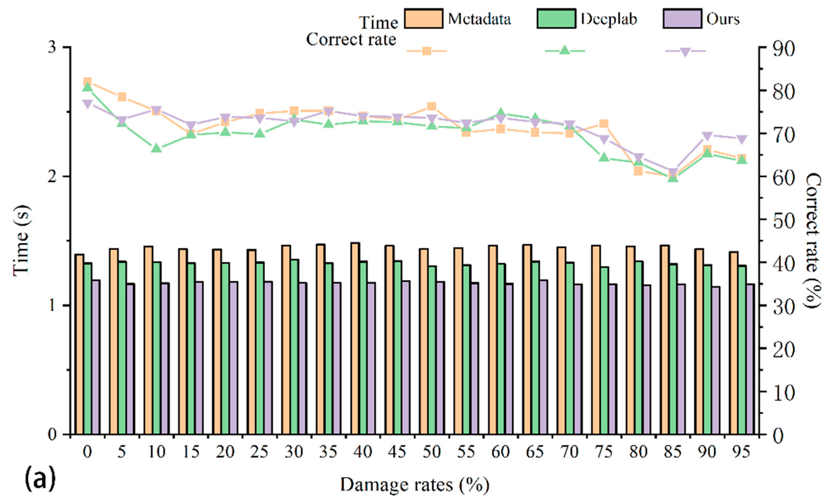
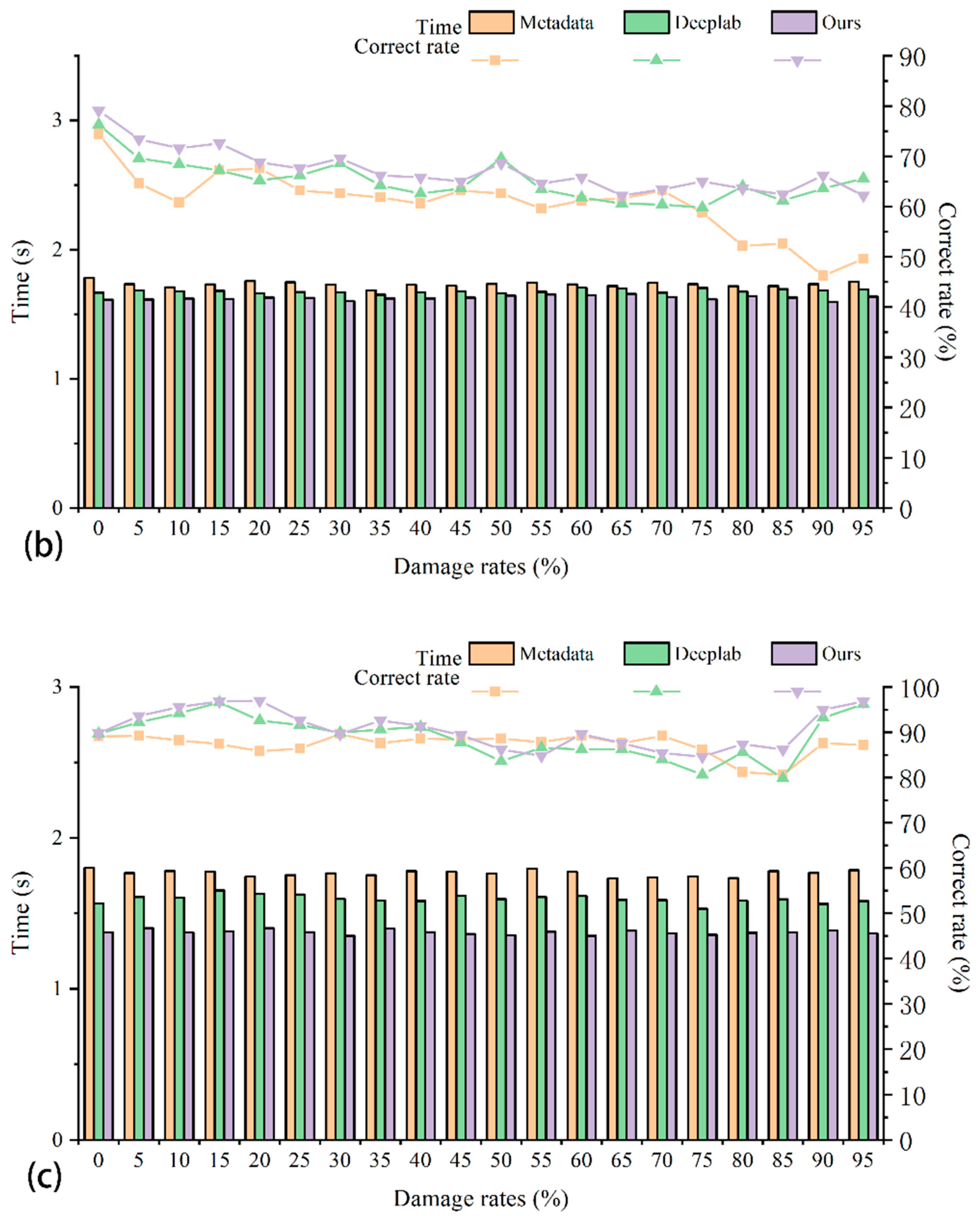
As shown in Figure 8, it can be concluded that as the number of images in the dataset increases, the final positioning time of several retrieval algorithms also increases. When using SIFT features and our deep learning feature points for localization, the time for retrieval and localization in the original database is significantly higher than the time for localization after semantic segmentation and screening of the dataset, while when using deep learning feature vectors for retrieval and localization, The time difference is not significant. This shows that reducing the number of datasets has a great effect on the retrieval and positioning time when using image feature points for retrieval and positioning tests. It can also illustrate that our method is more competitive in engineering applications at the metropolitan scale.

Effect on Positioning

The role of semantic segmentation in the whole localization process is to screen out images with too many interfering elements and less useful information, as shown in Figure 8. In Figure 8a–c, the retrieval effects of different retrieval methods on the pre-screened and post-screened datasets are basically similar, i.e., the method of reducing images with less useful information in the database by semantic segmentation has no or little effect on the retrieval and localization effects. It can be demonstrated that our method not only speeds up retrieval localization but also achieves better localization results without affecting the correct localization rate. These also prove the significance of our work.

3.4.3. Effectiveness of Improved Image Retrieval Algorithm

Reduce Storage

As shown in

Table 6. Memory size occupied by image retrieval and storage feature files.

	Dataset	Metadata	Deeplab_seg	Ours_seg
Feature
SIFT Feature		918 MB	807 MB	675 MB
Resnet		94.6 MB	82.9 MB	68.5 MB
R2D2 Feature		790 MB	693 MB	572 MB

, the neural network method of extracting feature vectors can effectively reduce the size of stored feature files. It can also be seen that the SIFT feature index requires more storage space, and from this point of view, our proposed deep learning-based feature point retrieval method outperforms the hand-crafted feature point extraction method.

The Effect on the Search Effect

In recent years, in the field of image recognition and matching, deep learning features often outperform artificial features. In Table 2, the results using deep learning features achieve higher accuracy than the experiments retrieved without deep learning methods. In all experiments, the highest value of almost every correct rate is obtained by our improved algorithm ours_r2d2.

Figure 9, Figure 10 and Figure 11 show the retrieval results of the query image in detail.

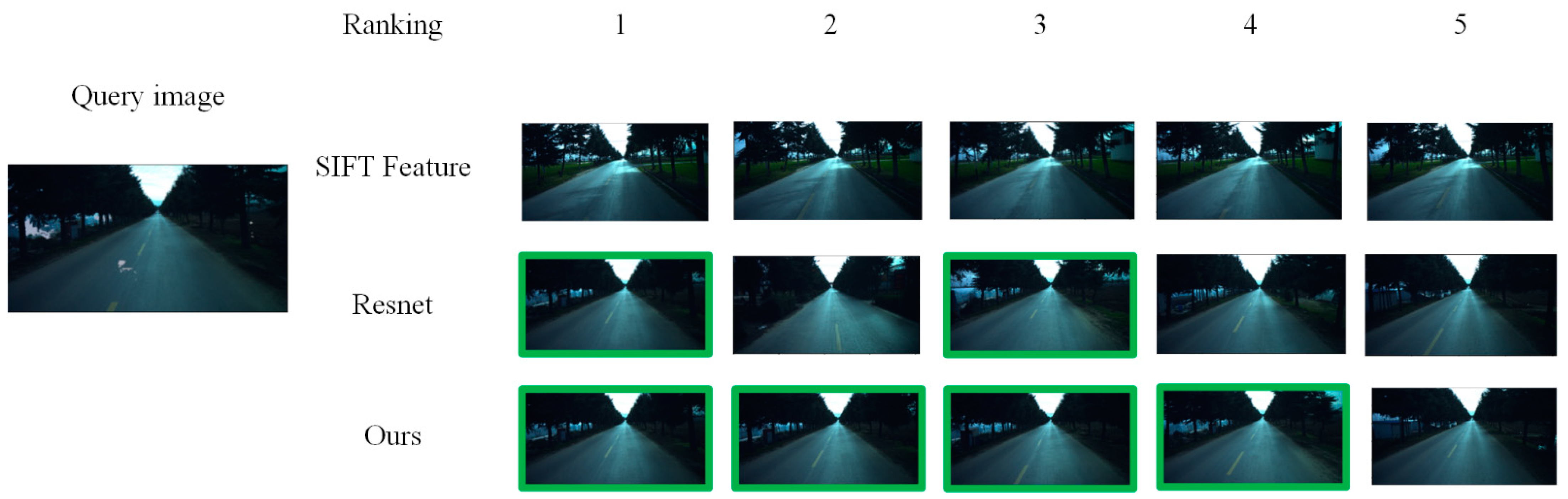
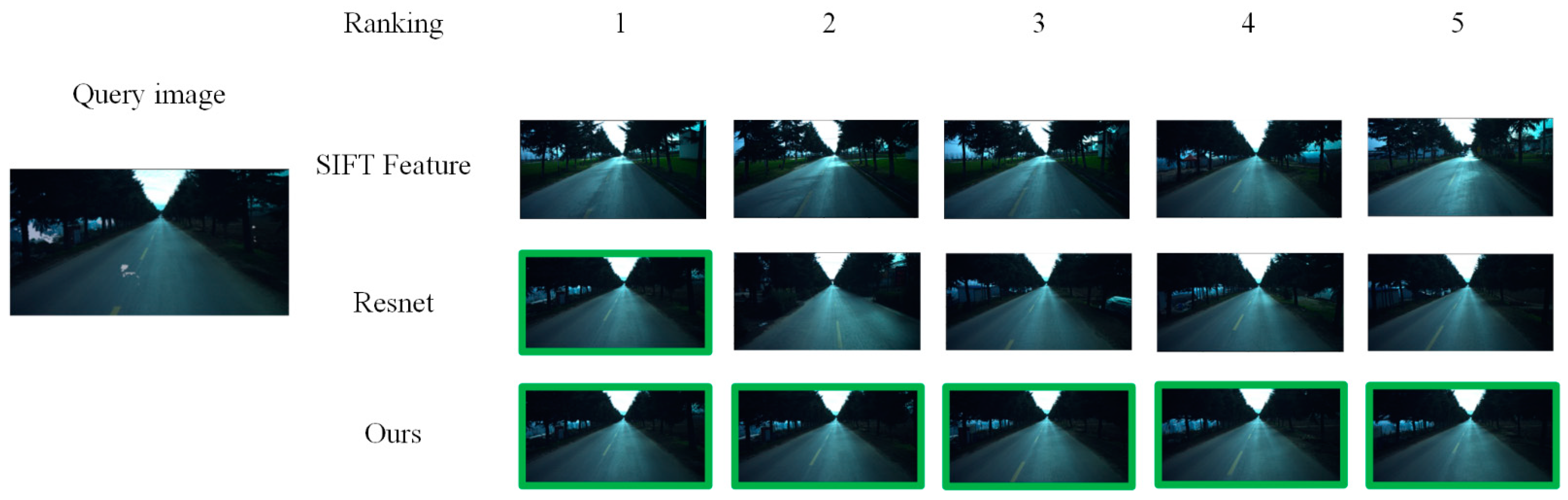
In Figure 9 and Figure 11, the localization task of the corrupted images is very difficult, and the top 5 retrieval results of SIFT and Resnet do not or only a few complete the localization task. However, after using our method, the retrieval of images was completed with correct results.

In Figure 9, Figure 10 and Figure 11, the result image of SIFT is not very similar to the original image. Additionally, in all search results, the correct result will be displayed in the top image list. According to the failure of SIFT feature retrieval caused by some damages in the figure, it shows that the damage area has great interference to SIFT features. This demonstrates the success of our adoption of deep learning feature points. The correct rate of retrieval results also proves the effectiveness of using deep learning feature points in adversarial damaged region retrieval.

This section may be divided by subheadings. It should provide a concise and precise description of the experimental results, their interpretation, as well as the experimental conclusions that can be drawn.

4. Conclusions

The goal of this paper is to perform geo-location in damaged road conditions. When dealing with the image-based localization task of damaged road sections, the existing methods do not specifically optimize the damaged road images in the feature extraction stage. Such complex scenes after buildings or road signs are damaged are not conducive to feature extraction. If the features extracted from the damaged image are used for matching, these features falling on meaningless objects will also affect the accuracy of the localization results. For this purpose, this paper describes a method for geo-location of damaged road images, which can achieve geo-location from non-geo-tagged to geo-tagged images in urban damaged areas. The method uses a variety of roadway images acquired by itself as the reference dataset constructs disturbed images using an improved semantic segmentation algorithm. An improved semantic segmentation algorithm is used to construct the disturbed images and use them as the damage dataset. The image localization task is accomplished by first rough geo-localization through image retrieval, and then fine geographic alignment through feature matching, thus adding accurate geotags to the damaged images. The main contribution of this paper is that the method has higher correctness and geo-localization speed than previous methods by using current road images and combining retrieval and matching algorithms, especially for road areas under damage and destruction conditions. Through experiments on the dataset, we fully demonstrate the effectiveness of the proposed algorithm and process. Compared with previous methods, our method improves the retrieval accuracy. Under the error requirement of 25 m, the correct rate of geolocation query images for damaged road images is higher than that of traditional algorithms. Our approach is very practical due to the metropolitan scale and data diversity of the datasets we use.