Performance Improvement of Image-Reconstruction-Based Defense against Adversarial Attack

Abstract

Deep Neural Networks (DNNs) used for image classification are vulnerable to adversarial examples, which are images that are intentionally generated to predict an incorrect output for a deep learning model. Various defense methods have been proposed to defend against such adversarial attacks, among which, image-reconstruction-based defense methods, such as DIPDefend, are known to be effective in getting rid of the adversarial perturbations injected in the image. However, this image-reconstruction-based defense approach suffers from a long execution time due to its iterative and time-consuming image reconstruction. The trade-off between the execution time and the robustness/accuracy of the defense method should be carefully explored, which is the main focus of this paper. In this work, we aim to improve the execution time of the existing state-of-the-art image-reconstruction-based defense method, DIPDefend, against the Fast Gradient Sign Method (FGSM). In doing so, we propose to take the input-specific properties into consideration when deciding the stopping point of the image reconstruction of DIPDefend. For that, we first applied a low-pass filter to the input image with various kernel sizes to make a prediction of the true label. Then, based on that, the parameters of the image reconstruction procedure were adaptively chosen. Experiments with 500 randomly chosen ImageNet validation set images show that we can obtain an approximately 40% improvement in execution time while keeping the accuracy drop as small as 0.4–3.9%.

1. Introduction

As research on deep learning has become active in recent years, DNNs [1] have been used in various fields, such as image classification, object detection [2], detecting the edge information of a high-resolution image [3,4] and Natural Language Processing (NLP) [5]. In particular, DNNs surpassed human performance in some tasks. However, these DNNs are known to be vulnerable to adversarial attacks. An adversarial attack is an attack that adds adversarial perturbation that causes the neural network to malfunction, while the attacked image cannot be distinguished by human visual recognition. Such adversarial attacks are hard to notice because the attacked image not only has robust features that human can distinguish well, such as cat ears and tails, but also non-robust features that are hardly noticeable by human vision. These can be fatal in cases where DNNs can cause serious problems in safety-related applications, such as self-driving cars [6] and medical devices [7,8,9].

In the past few years, as research on adversarial attacks has become active, several defense methods against these attacks have been proposed. There are two types of adversarial attacks, evasion and poisoning attacks, which are carried out in the test phase and training phases, respectively [10]. Examples of evasion attack include the Fast Gradient Sign Method (FGSM) [11] and Projected Gradient Descent (PGD) [12], whereas BadNets [13] is a poisoning attack. The most representative defense method against adversarial attacks is adversarial training [11], in which, a retraining is performed with a new training dataset that includes attacked adversarial examples with their true labels. There have also been several defense methods proposed to enhance the robustness of DNNs [14,15,16].

Dai et al. [17] proposed a unique approach called DIPDefend that does not enhance the DNN model but makes it reliable by reconstructing the input image. Such reconstruction-based defense methods usually have a trade-off between the accuracy and execution time. That is, it takes a longer time to reconstruct images in order to make it more reliable against adversarial attacks. While images have different properties in practice, DIPDefend does not considered these individual characteristics and simply assumes the same set of fitting coefficients, as will be shown in Section 2. In this work, on the other hand, we considered individual characteristics of the input image, based on which, the image reconstruction time is significantly reduced while keeping the accuracy reduction minimal.

2. Related Work

In this section, we describe an evasion attack, which we consider in this paper as a target adversarial attack, and image reconstruction, which we rely on as a defense against evasion attacks.

2.1. Evasion Attack

An evasion attack is one of the most common attacks in deep learning. This attack does not affect the training data but manipulates the test data during the testing phase to cause the neural network to predict an incorrect output. The manipulated images are referred to as adversarial examples. Table 1 [18] explains why evasion attacks are so successful. An adversarial example is created by adding adversarial perturbation to the original image, which consists of high-frequency (non-robust) features. That is, it can be said that adversarial examples are created by mainly manipulating non-robust features that are not easily distinguished by human vision. This is why it is not trivial to distinguish whether an image is attacked or not only with human visual inspection. In this paper, we used FGSM [11], which supports the fast generation of adversarial examples using the linearity of a deep neural network model.

Table 1. Image components.

Image Components	Feature
Robust Features	Characteristics that can be distinguished by human Low-Frequency E.g., tails of animals, ears of animals, etc.
Non-Robust Features	Characteristics that human cannot be distinguished well High-Frequency E.g., hair whorl of animals, etc.

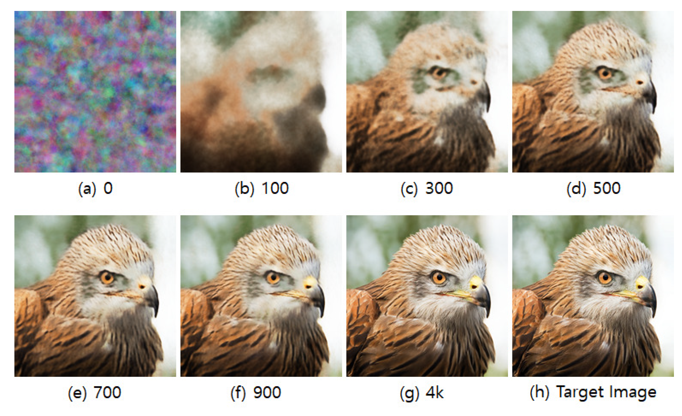
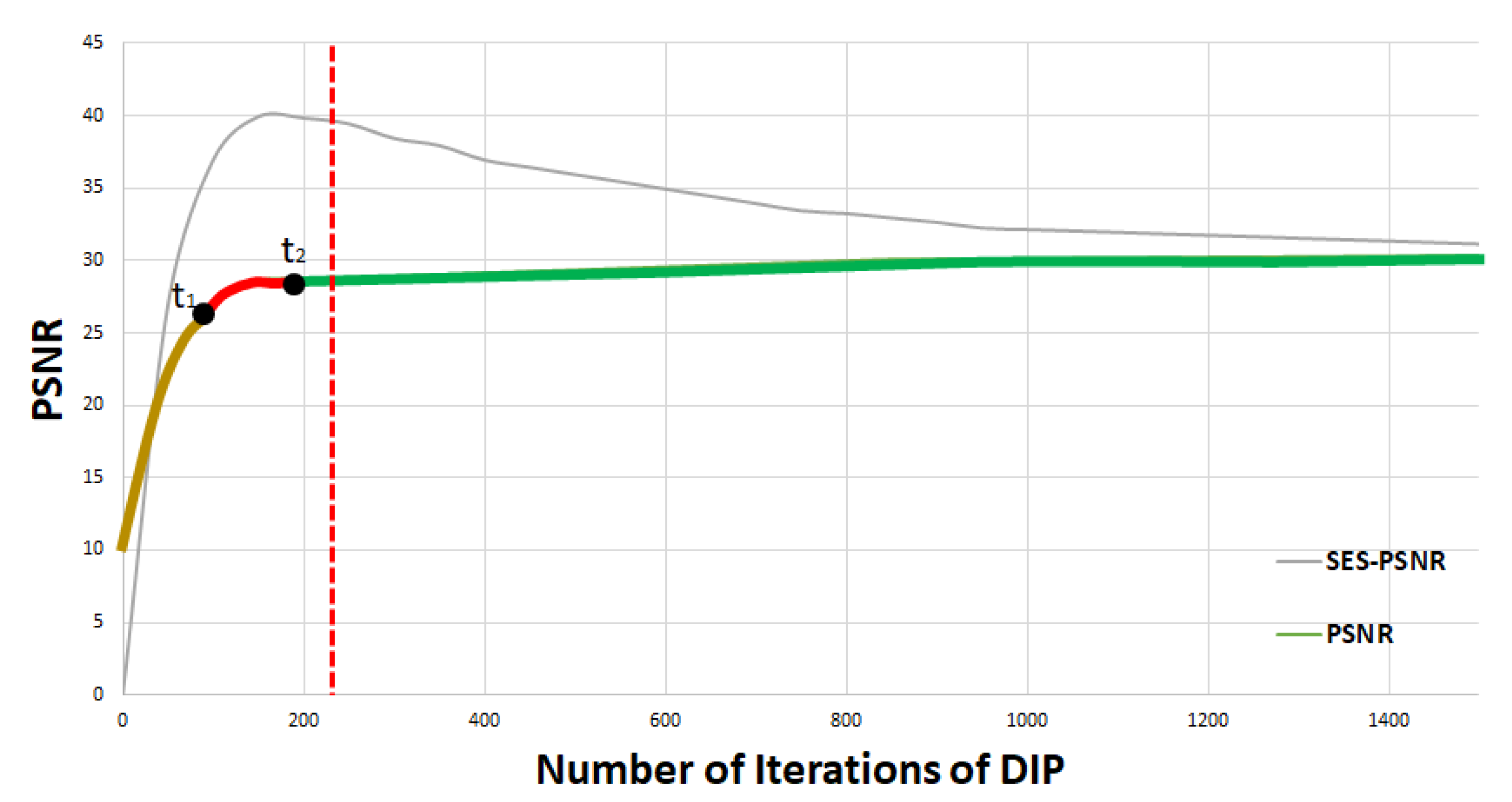
2.2. Deep Image Prior (DIP)

Deep Image Prior (DIP) [19] is an image reconstruction method that starts with random noise and reconstructs an image in an iterative way, gradually making it closer to the target image. In addition, DIP utilizes features of Convolutional Neural Networks (ConvNets) architecture to capture low-level features from images without training. Figure 1 shows the results of various image reconstruction methods for a noise-added image in comparison. It can be seen, even with human vision, that DIP could reconstruct the details (high-frequency features) of the image well compared to others.

Figure 1. Comparison of reconstructed images: (a) original image with noise, (b) low-pass filtered image, (c) reconstructed image using VDSR [20], and (d) reconstructed image using DIP.

Figure 2 illustrates the iterative procedure of DIP. It starts from a randomly initialized ConvNet (${\theta }_0$) that reconstructs an image from a randomly generated noise (z). DIP iteratively updates the ConvNet weights $\theta$ in a way so that the generated image is as close as possible to the target image $x_t$.

Figure 2. Overall procedure of DIP.

Figure 3 shows the example reconstructed images for different numbers of iterations in DIP. Comparing the reconstructed image after 700 iterations, Figure 3e, with the target image, Figure 3h, it can be seen that the image under reconstruction has much fewer high-frequency features (noise). This means that DIP can also be used to remove high-frequency features (noise). Thus, if one can decide on the number of iterations where only the robust features are reconstructed, DIP can successfully be used to filter out the injected perturbation in adversarial examples.

Figure 3. Image reconstruction by the number of DIP iterations.

Figure 4 shows how DIP can be used to defend against adversarial attacks. The image to be reconstructed in Figure 4 is an adversarial example $x_{adv}$ generated by an adversarial attack. The iterations of DIP can be divided into three stages. First, the image (between $t_0$ and $t_1$) is reconstructed, starting from random noise, independent of both the adversarial example $x_{adv}$ and the original image $x_{gt}$. In the second stage (between $t_1$ and $t_2$), the reconstructed image is similar to $x_{gt}$, with only robust features reconstructed out of $x_{adv}$. Lastly, the image generated later than $t_2$ contains abundant non-robust features in which adversarial perturbation is hidden. Therefore, it is important to determine the second stage ($t_1$ and $t_2$), during which, only robust features are reconstructed, in order to successfully filter out perturbation from an adversarial example.

Figure 4. DIP image reconstruction of an adversarial example.

DIPDefend [17] uses Second-order Exponential Smoothing (SES)-PSNR, a method of measuring PSNR trends in reconstructed images to determine the second stage ($t_1$ and $t_2$). This is a method that utilizes the fact that PSNR increases rapidly when reconstructing the robust features because most of the energy in the image is contained at a low frequency. Therefore, the point until which PSNR has risen rapidly and stopped increasing suddenly is most likely between $t_1$ and $t_2$, and this is the point where DIP needs to stop its iterations. Figure 5 shows how SES-PSNR and PSNR change as the number of iterations of DIP increases. In Figure 5, PSNR increases as it reconstructs the robust features in the early stages of DIP iteration, which tends to converge after $t_2$. Based on this, when the peak of SES-PSNR is found (between $t_1$ and $t_2$), DIPDefend stops reconstructing the image. SES-PSNR, denoted as $s_t$, can be obtained using Equation (1). Since there is no ground-truth image (i.e., original unattacked image) available, PSNR, denoted as $p_t$, is calculated using an adversarial example. $b_t$ used in Equation (1) represents a change in the tendency of the previous cycle and can be obtained using Equation (2).

$$s_t=\alpha ·p_t+(1-\alpha )·(s_{t-1}+b_{t-1})$$

(1)

$$b_t=\beta ·(s_t-s_{t-1})+(1-\beta )·b_{t-1}$$

(2)

Figure 5. SES-PSNR and PSNR by DIP iterations.

There are fitting coefficients $\alpha$ and $\beta$ in the above equations. Note that the most appropriate values for $\alpha$ and $\beta$ may differ from one adversarial example to another. In DIPDefend, these values are empirically determined and have been used for all images.

3. Proposed Method

This section describes the proposed technique that enhances the DIP-based defense against adversarial attacks. In particular, it presents how to shorten the average execution time taken for image reconstruction by choosing the stopping point individually for each image.

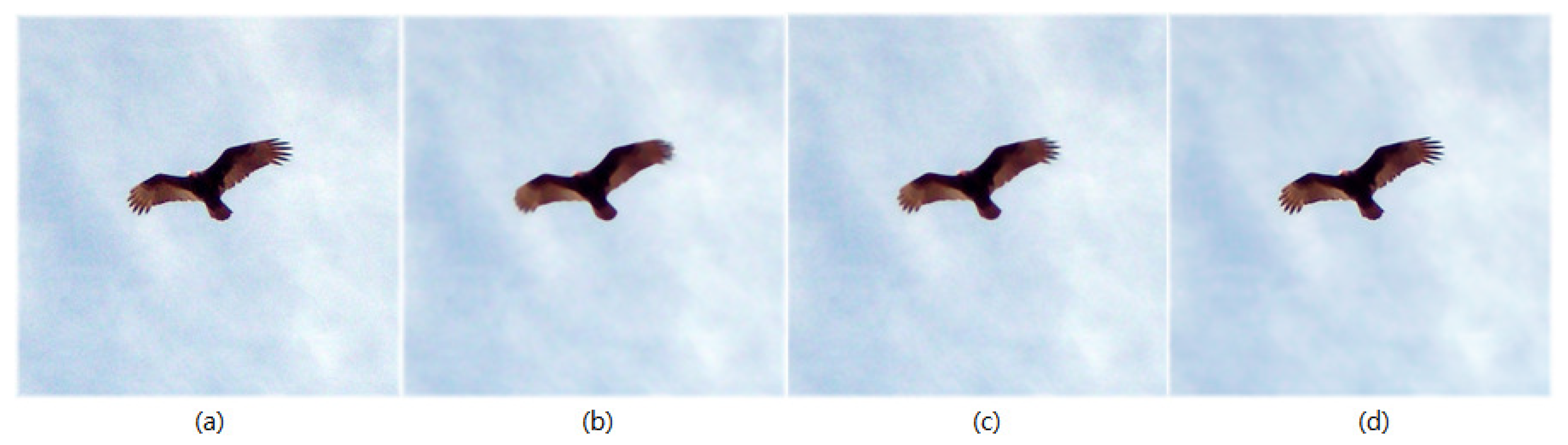
3.1. Searching for Ground-Truth Label Using Low-Pass Filter (LPF)

As stated earlier, each input image may have different property itself. Moreover, the degree of adversarial attack may also be different. In the proposed technique, we accounted for such individual properties by applying Low-Pass Filter (LPF) [21] to the input image before entering into the reconstruction stage. Typically, by applying LPF, an image is smoothed. That is, each pixel value is replaced with a weighted sum of neighboring pixels and the square grid that defines the weights of neighboring pixels is called kernel. For example, an LPF with a kernel size of 3 smoothens each pixel considering its $3\times 3$ surrounding pixels.

In order to illustrate how LPF could be used to defend against adversarial attacks, we observed how low-pass filtered adversarial images affect the accuracy of classification. For that, we used ResNet50 [22] and 500 randomly chosen images from ImageNet [1] validation set. Table 2, Table 3 and Table 4 report the accuracy of image classifications from adversarial examples generated with $ϵ$ of 2, 8, and 16 using FGSM, respectively. Note that $ϵ$ in FGSM can be seen as the degree of attack, i.e., a bigger $ϵ$ indicates a stronger attack. In each case, we varied the kernel size of LPF. These results show that LPF can slightly remove the adversarial perturbations hidden in features that are non-robust.

Table 2. Accuracy when applying an LPF to adversarial example of $ϵ$ = 2.

Kernel Size	No LPF	3	5	7	9	11	13
Accuracy (%)	17.4	55.2	57.8	55.2	47.8	38.8	33.0

Table 3. Accuracy when applying an LPF to adversarial example of $ϵ$ = 8.

Kernel Size	No LPF	3	5	7	9	11	13
Accuracy (%)	3.0	34.4	47.4	48.2	42.4	35.4	32.2

Table 4. Accuracy when applying an LPF to adversarial example of $ϵ$ = 16.

Kernel Size	No LPF	3	5	7	9	11	13
Accuracy (%)	2.4	20.6	35.6	38.6	36.2	32	27.8

As shown in the above results, the accuracy of the low-pass filtered adversarial examples depends on the kernel size. In addition, the size of the kernel with the highest accuracy depends on the $ϵ$. That is, the optimal kernel size was different for the three $ϵ$ values. This observation supports that it is important to take individual properties into consideration in the defense against adversarial attacks. Due to this difficulty, applying LPF cannot solely be a defense method by itself. Rather, in the proposed method, we used LPF to obtain a predicted label, which was used to optimize the execution time of image-reconstruction-based defense method later on (as is shown in Section 3.3).

Generally speaking, it tends to remove high frequency features of the image more aggressively as the kernel size of LPF gets bigger. Thus, we performed inferences iteratively on the low-pass filtered images while gradually increasing the kernel size from the smallest one. Then, we examined how the inference result changes over the varying kernel sizes. Firstly, we observed how many images result in no changes while varying the kernel size. As reported in Table 5, it has been observed that the lower the degree of attack, i.e., $ϵ$, the more proportions of images did not result in changes in the inference. To be more specific, approximately a third of the randomly chosen images did not show any changes in the inference results while varying the kernel size of LPF. For the other cases, we empirically observed that the probability that the first changed label we obtain by varying the kernel size of LPF happens to be the true label is approximately 5–6 times higher than that of the second (or later) changed label.

Table 5. Portion of images whose inference results do not change over the LPF kernel size changes.

Attack	No Attack	$\mathit{ϵ}=2$	$\mathit{ϵ}=8$	$\mathit{ϵ}=16$
Ratio (%)	32	32.4	25.6	18.2

3.2. Different Parameters for DIPDepend

DIPDefend [17] uses constant $\alpha$ and $\beta$ values for all examples to determine when to stop the DIP iteration. In order to illustrate the necessity of individual choice of coefficient in DIPDefend, we observed how different values of $\alpha$ and $\beta$ affect the accuracy of classification for adversarial examples. Again, we used ResNet50 [22] and 500 randomly chosen images from ImageNet [1] validation set for this experiment. Table 6, Table 7 and Table 8 show the average accuracy for the 500 randomly chosen images when $ϵ$ is 2, 8, and 16, respectively. To be more specific, we tested the following for coefficient choices:

Table 6. Accuracy when applying DIPDefend to adversarial examples of $ϵ$ = 2.

($\mathit{\alpha }$, $\mathit{\beta }$)	(0.01, 0.01)	(0.01, 0.001)	(0.001, 0.01)	(0.001, 0.001)
Accuracy (%)	13.0	38.6	49.2	65.4

Table 7. Accuracy when applying DIPDefend to adversarial examples of $ϵ$ = 8.

($\mathit{\alpha }$, $\mathit{\beta }$)	(0.01, 0.01)	(0.01, 0.001)	(0.001, 0.01)	(0.001, 0.001)
Accuracy (%)	13.4	38.0	48.2	61.8

Table 8. Accuracy when applying DIPDefend to adversarial examples of $ϵ$ = 16.

($\mathit{\alpha }$, $\mathit{\beta }$)	(0.01, 0.01)	(0.01, 0.001)	(0.001, 0.01)	(0.001, 0.001)
Accuracy (%)	13.4	34.4	45.8	52.2

• Mode 1: $\alpha =0.01$, $\beta =0.01$;
• Mode 2: $\alpha =0.01$, $\beta =0.001$;
• Mode 3: $\alpha =0.001$, $\beta =0.01$;
• Mode 4: $\alpha =0.001$, $\beta =0.001$.

As can be seen in the tables, the smaller the values of $\alpha$ and $\beta$, the higher the accuracy that could be obtained.

The improved accuracy, however, comes at the cost of increased image reconstruction time. Table 9 reports that smaller $\alpha$ and $\beta$ values result in bigger number of DIP iterations until stopping; thus, larger reconstruction time in DIPDefend. In other words, one has to explore a trade-off between reliability (accuracy) and execution time (taken for defense) when applying DIPDefend as a measure against adversarial attacks. Optimal choice of $\alpha$ and $\beta$ must be dependent upon the individual characteristics of the input image and the degree of attack, i.e., $ϵ$ in FGSM.

Table 9. Average number of DIP iterations taken for reconstruction for different $\alpha$ and $\beta$.

($\mathit{\alpha }$, $\mathit{\beta }$)	(0.01, 0.01)	(0.01, 0.001)	(0.001, 0.01)	(0.001, 0.001)
Number of DIP iterations	250	583	923	2514

In order to show the effectiveness of individually chosen coefficients of DIPDefend, we conducted the following experiment. For each input image, we tried all four combinations of $\alpha$ and $\beta$ listed above and considered them to be accurate if any of them inferred a correct label. In other words, we assumed that there is a method to choose ideal coefficient among the four and examine the highest achievable accuracy from this ideal choice. Table 10 reports the average accuracy of such ideal $\alpha$ and $\beta$ for 500 randomly chosen adversarial examples.

Table 10. Accuracy when applying ideal $\alpha$ and $\beta$.

$\mathit{ϵ}$	2	8	16
Accuracy(%)	69.2	66.4	61.8

Note that the accuracy of Table 10 (ideal choice of $\alpha$ and $\beta$) is higher than the cases with constant $\alpha =0.001$ and $\beta =0.001$ of Table 6, Table 7 and Table 8. This indicates that the smallest $\alpha$ and $\beta$ do not always result in the optimal defense. In what follows, we propose a method for reducing the image reconstruction time in DIPDefend while keeping the accuracy degradation minimal by choosing appropriate $\alpha$ and $\beta$ individually for each image.

3.3. Algorithm of Proposed Method

The proposed method consists of two different stages. First, we predicted the original (unattacked) label of the input image by applying LPF (Algorithm 1). Then, based on that, we tried to apply a suitable $\alpha$ and $\beta$ adaptively to reduce the image reconstruction time in Algorithm 2.

As stated in Section 3.1, some adversarial perturbations can be mitigated by applying LPF. As we do not know the degree of attack, we started from a small kernel size, 3, and gradually increased it to 13, applying LPF to the input example iteratively. Recall that our observation in Section 3.1 is that either the inferred label never changes or the first changed label is much likely to be the correct label as we increase the kernel size of LPF that is applied to the input image. In line with this, Algorithm 1 initializes its prediction to be the inference result made from the low-pass filtered image with kernel size of 3 (line 5). Then, we performed the inferences repeatedly as the kernel size of LPF gradually increased (lines 6–7). Whenever the inference result deviates from the initial prediction for the first time (line 8), we considered this as a predicted label. Otherwise, we just kept the initial prediction (line 13).

Algorithm 1 Prediction of the original label.

1: $x_{adv}$: Input image 2: $M(x_{adv},N)$: A new image obtained by applying LPF with kernel size N to $x_{adv}$ 3: $Y_N$: Inferred label of $M(x_{adv},N)$ 4:   5: $Y_3\leftarrow$ Inference result of $M(x_{adv},3)$ 6: forN in 5 to 13 do 7:     $Y_N\leftarrow$ Inference result of $M(x_{adv},N)$ 8:     if if $Y_3\ne Y_N$ then 9:         return $Y_N$ 10:     end if 11:     $N\leftarrow N+2$ 12: end for 13: return$Y_3$

Based on the prediction made by Algorithm 1, we determined a suitable set of parameters ($\alpha$ and $\beta$) that can reduce the execution time of the defense method while maintaining robustness. While we consider the following four modes in this work, it is worthwhile to mention that the proposed method can be applied to more parameters without loss of generality:

• Mode 1: $\alpha =0.01$, $\beta =0.01$,
• Mode 2: $\alpha =0.01$, $\beta =0.001$,
• Mode 3: $\alpha =0.001$, $\beta =0.01$, and
• Mode 4: $\alpha =0.001$, $\beta =0.001$.

The main idea is that we first try the defense from the biggest $\alpha$ and $\beta$ values (in this case mode 1) in favor of reduced execution time. Then, we check if the result obtained from this value is good enough by comparing the inference result with the predicted label. If this is good, we make an early termination; otherwise, we move on to the next values, which are smaller than the current parameters. This is how we propose to explore the trade-off between execution time and robustness (accuracy) in the image-reconstruction-based defense.

Algorithm 2 delineates this procedure. It starts by making a prediction of the label by invoking Algorithm 1 (line 8). Then, starting from mode 1 (the biggest $\alpha$ and $\beta$ (line 9)), it applies DIPDefend (lines 10–16). Whenever a SES-PSNR peak is found as the iteration continues (line 17), it examines whether the current reconstructed image results in the same inference result as the predicted one (line 18). If the current inference is the same as the predicted one, we terminate the DIP procedure early (line 19). If not, the $\alpha$ and $\beta$ values are updated with the next ones, with which, we start over a new DIPDefend procedure (line 21; by terminating the inner for loop, the next iteration of the outer for loop continues). When the peak is found in the last mode (mode 4 in this case), the entire procedure stops (line 18). As can be seen in the pseudocode, the algorithm has two nested for loops; thus, its time complexity is $O(N·T)$, where N and T denote the number of considered modes and the maximum number of image reconstruction steps, respectively.

Algorithm 2 Inference with adaptive $\alpha$ and $\beta$.

1: z: Random noise 2: $x_t$: Reconstructed image at iterations t 3: $p_t$: PSNR calculated from $x_t$ against $x_{adv}$ 4: $s_t$: SES-PSNR calculated for $x_t$ 5: $f_t$: DIP neural network at iteration t 6: $Y_p$: Predicted label by applying LPF 7:   8: $Y_p\leftarrow$ Algorithm 1                        ▹ Label prediction 9: for$n\leftarrow 1$ to 4 do                   ▹ From mode 1 to mode 4 10:     $x_0\leftarrow z,p_t\leftarrow 0,s_t\leftarrow 0,x_0\leftarrow f_t\left(x_0\right)$           ▹ DIP initialization 11:     for $t\leftarrow 0$ to ∞do                      ▹ DIP iterations 12:         $Y_t\leftarrow$ Inference result of $x_t$ 13:         $x_{t+1}\leftarrow f_t\left(x_t\right)$ 14:         $p_{t+1}\leftarrow PSNR$ 15:         $s_{t+1}\leftarrow \alpha ·p_{t+1}+(1-\alpha )·(s_t+b_t)$          ▹ Calculate SES-PSNR 16:         $b_{t+1}\leftarrow \beta ·(s_{t+1}-s_t)+(1-\beta )·b_t$ 17:         if $s_{t+1}$ < $s_t$ then               ▹ If a peak in SES-PSNR found 18:            if $Y_p=Y_t$ or $n=4$ then   ▹ coincides with the predicted label or mode 4 19:                return $Y_t$ 20:            else 21:                break                         ▹ To the next mode 22:            end if 23:         end if 24:     end for 25: end for

4. Evaluation

In this section, we present the experimental results that evaluate the proposed method in terms of the accuracy and execution time.

4.1. Experimental Settings

The neural network used to evaluate the proposed defense method was ResNet50 [22], which used a randomly selected 500 ImageNet [1] dataset. Figure 6 shows how the inference accuracy drops as the degree of FGSM attack $ϵ$ increases. The $ϵ$ values that we use in the following evaluations and their corresponding accuracies are summarized in Table 11.

Figure 6. Accuracy drop with various $ϵ$ values.

Table 11. Various $ϵ$ values used in the experiments and the average classification accuracy of attacked images in each $ϵ$.

$\mathit{ϵ}$	0 (No Attack)	2	8	16
Accuracy (%)	72.2	17.4	3.0	2.4

4.2. Results on the Accuracy and Performance

Table 12 compares the accuracy and execution time between DIPDefend and the proposed method of $ϵ$ = 2. DIPDefend achieves a maximum accuracy of 65.4% in mode 4 ($\alpha$ = 0.001, $\beta$ = 0.001), whereas the proposed method achieves an accuracy of 62.6%; the accuracy drop by the proposed method is 2.8%. However, the execution time taken for reconstruction could be significantly reduced from 224 s to 143.2 s by the proposed method (the execution time improvement is 41.3%).

Table 12. Execution time and accuracy of DIPDefend and the proposed method when $ϵ$ = 2.

DIPDefend					Proposed Method
($\mathit{\alpha }$, $\mathit{\beta }$)	(0.01, 0.01)	(0.01, 0.001)	(0.001, 0.01)	(0.001, 0.001)
Accuracy (%)	13.0	38.6	49.2	65.4	62.6
Execution Time (s)	24.30	56.52	89.49	244.0	143.2

We repeated the same experiment for $ϵ$ = 8 and $ϵ$ = 16, whose results are presented in Table 13 and Table 14, respectively. The same tendency was observed for both cases.

Table 13. Execution time and accuracy of DIPDefend and the proposed method when $ϵ$ = 8.

DIPDefend					Proposed Method
($\mathit{\alpha }$, $\mathit{\beta }$)	(0.01, 0.01)	(0.01, 0.001)	(0.001, 0.01)	(0.001, 0.001)
Accuracy (%)	13.4	38	48.2	61.8	60
Execution Time (s)	24.26	56.40	89.41	243.6	135.1

Table 14. Execution time and accuracy of DIPDefend and the proposed method when $ϵ$ = 16.

DIPDefend					Proposed Method
($\mathit{\alpha }$, $\mathit{\beta }$)	(0.01, 0.01)	(0.01, 0.001)	(0.001, 0.01)	(0.001, 0.001)
Accuracy (%)	13.4	34.4	45.8	52.2	51.8
Execution Time (s)	24.15	56.33	89.13	242.0	145.6

Table 15 summarizes the peformance of DIPDefend and the proposed method in comparison. It could be observed that the proposed method results in a smaller accuracy drop as the degree of attack ($ϵ$) increases while preserving the performance improvement as significant as approximately $40\%$.

Table 15. Comparison between DIPDefend and the proposed method with adversarial examples.

$\mathit{ϵ}$	2		8		16
Defense Method	DIPDefend	Proposed Method	DIPDefend	Proposed Method	DIPDefend	Proposed Method
Accuracy (%)	65.4	62.6	61.8	60	52.2	51.8
Accuracy drop (%)	2.8		1.8		0.4
Execution time (s)	244.0	143.2	243.6	135.1	242.0	145.6
Exec. improvement (%)	41.3		44.5		39.8

Lastly, we verified that the proposed method still remains effective in the case where the input image has not been attacked. We repeated the same experiment with the same set of images, but, this time, no adversarial attacks were applied to them. Table 16 compares the accuracy and execution time of the proposed method with those of DIPDefend to the original image without an adversarial attack.

Table 16. Comparison between DIPDefend and the proposed method with original (unattacked) images.

Defense Method	DIPDefend	Proposed Method
Accuracy (%)	66.0	62.1
Accuracy drop (%)	3.9
Execution time (s)	243.8	158.8
Exec. improvement (%)	34.9

5. Conclusions

In this paper, we proposed an improved image-reconstruction-based defense method against adversarial attacks The existing image-reconstruction-based defense methods, such as DIPDefend, need to determine the number of iterations taken to reconstruct images before inference. In doing so, they have considered neither individual characteristics of input images nor the degree of attack. Thus, they needed to have constant and conservative parameters ($\alpha$ and $\beta$) for determining the stop point of image reconstruction, for which, the execution time for defense was significant. On the contrary, the proposed method takes an adaptive approach to determine the stopping point of image reconstruction. Firstly, we propose applying low-pass filters with various kernel sizes to roughly predict the true label. Then, based on this, we tried to run DIPDefend with more efficient parameters that allow for faster image reconstruction. If the intermediate result was good enough, i.e., identical to the predicted label, we stopped the image reconstruction early in favor of a reduced defense execution time. With 500 randomly chosen images from the validation set of ImageNet, it has been shown that the proposed method could obtain up to a 44.5% improvement in execution time against the basic DIPDefend while keeping the accuracy drop as small as 0.4–3.9%.

References

- Krizhevsky, A.; Sutskever, I.; Hinton, G.E. Imagenet classification with deep convolutional neural networks. Adv. Neural Inf. Process. Syst. 2012, 25, 1097–1105. [Google Scholar] [CrossRef]
- Zhao, Z.Q.; Zheng, P.; Xu, S.T.; Wu, X. Object detection with deep learning: A review. IEEE Trans. Neural Netw. Learn. Syst. 2019, 30, 3212–3232. [Google Scholar] [CrossRef] [PubMed] [Green Version]
- Chen, Z.; Luo, X. Fuzzy Control Method for Synchronous Acquisition of High Resolution Image based on Machine Learning. Int. J. Circuits Syst. Signal Process. 2022, 16, 363–373. [Google Scholar] [CrossRef]
- Shylashree, N.; Anil Naik, M.; Sridhar, V. Design and Implementation of Image Edge Detection Algorithm on FPGA. Int. J. Circuits Syst. Signal Process. 2022, 16, 628–636. [Google Scholar] [CrossRef]
- Chowdhary, K. Natural language processing. In Fundamentals of Artificial Intelligence; Springer: Berlin/Heidelberg, Germany, 2020; pp. 603–649. [Google Scholar]
- Bojarski, M.; Testa, D.D.; Dworakowski, D.; Firner, B.; Flepp, B.; Goyal, P.; Jackel, L.D.; Monfort, M.; Muller, U.; Zhang, J.; et al. End to End Learning for Self-Driving Cars. arXiv 2016, arXiv:abs/1604.07316. [Google Scholar]
- Esteva, A.; Robicquet, A.; Ramsundar, B.; Kuleshov, V.; DePristo, M.; Chou, K.; Cui, C.; Corrado, G.; Thrun, S.; Dean, J. A guide to deep learning in healthcare. Nat. Med. 2019, 25, 24–29. [Google Scholar] [CrossRef] [PubMed]
- Caridade, C.M.R.; Roseiro, L. Automatic Segmentation of Skin Regions in Thermographic Images: An Experimental Study. WSEAS Trans. Signal Process. 2021, 17, 57–64. [Google Scholar]
- Vetova, S. A Comparative Study of Image Classification Models using NN and Similarity Distance. WSEAS Trans. Int. J. Electr. Eng. Comput. Sci. 2021, 3, 109–113. [Google Scholar]
- Chakraborty, A.; Alam, M.; Dey, V.; Chattopadhyay, A.; Mukhopadhyay, D. Adversarial attacks and defences: A survey. arXiv 2018, arXiv:1810.00069. [Google Scholar] [CrossRef]
- Goodfellow, I.J.; Shlens, J.; Szegedy, C. Explaining and harnessing adversarial examples. arXiv 2014, arXiv:1412.6572. [Google Scholar]
- Madry, A.; Makelov, A.; Schmidt, L.; Tsipras, D.; Vladu, A. Towards deep learning models resistant to adversarial attacks. arXiv 2017, arXiv:1706.06083. [Google Scholar]
- Gu, T.; Dolan-Gavitt, B.; Garg, S. Badnets: Identifying vulnerabilities in the machine learning model supply chain. arXiv 2017, arXiv:1708.06733. [Google Scholar]
- Goel, A.; Agarwal, A.; Vatsa, M.; Singh, R.; Ratha, N.K. DNDNet: Reconfiguring CNN for adversarial robustness. In Proceedings of the IEEE/CVF Conference on Computer Vision and Pattern Recognition Workshops, Seattle, WA, USA, 13–19 June 2020; pp. 22–23. [Google Scholar]
- Ye, S.; Xu, K.; Liu, S.; Cheng, H.; Lambrechts, J.H.; Zhang, H.; Zhou, A.; Ma, K.; Wang, Y.; Lin, X. Adversarial robustness vs. model compression, or both? In Proceedings of the IEEE/CVF International Conference on Computer Vision, Montreal, BC, Canada, 11–17 October 2019; pp. 111–120. [Google Scholar]
- Xu, W.; Evans, D.; Qi, Y. Feature squeezing: Detecting adversarial examples in deep neural networks. arXiv 2017, arXiv:1704.01155. [Google Scholar]
- Dai, T.; Feng, Y.; Wu, D.; Chen, B.; Lu, J.; Jiang, Y.; Xia, S.T. DIPDefend: Deep Image Prior Driven Defense against Adversarial Examples. In Proceedings of the 28th ACM International Conference on Multimedia, Seattle, WA, USA, 12–16 October 2020; pp. 1404–1412. [Google Scholar]
- Ilyas, A.; Santurkar, S.; Tsipras, D.; Engstrom, L.; Tran, B.; Madry, A. Adversarial examples are not bugs, they are features. arXiv 2019, arXiv:1905.02175. [Google Scholar]
- Ulyanov, D.; Vedaldi, A.; Lempitsky, V. Deep image prior. In Proceedings of the IEEE Conference on Computer Vision and Pattern Recognition, Salt Lake City, UT, USA, 18–23 June 2018; pp. 9446–9454. [Google Scholar]
- Dong, C.; Loy, C.C.; He, K.; Tang, X. Image super-resolution using deep convolutional networks. IEEE Trans. Pattern Anal. Mach. Intell. 2015, 38, 295–307. [Google Scholar] [CrossRef] [PubMed] [Green Version]
- Selesnick, I.W.; Graber, H.L.; Pfeil, D.S.; Barbour, R.L. Simultaneous Low-Pass Filtering and Total Variation Denoising. IEEE Trans. Signal Process. 2014, 62, 1109–1124. [Google Scholar] [CrossRef]
- He, K.; Zhang, X.; Ren, S.; Sun, J. Deep residual learning for image recognition. In Proceedings of the IEEE Conference on Computer Vision and Pattern Recognition, Las Vegas, NV, USA, 27–30 June 2016; pp. 770–778. [Google Scholar]
Publisher’s Note: MDPI stays neutral with regard to jurisdictional claims in published maps and institutional affiliations. |
© 2022 by the authors. Licensee MDPI, Basel, Switzerland. This article is an open access article distributed under the terms and conditions of the Creative Commons Attribution (CC BY) license (https://creativecommons.org/licenses/by/4.0/).