Abstract
Aiming at the scarcity of Low Earth Orbit (LEO) satellite spectrum resources, this paper proposes an algorithm of interference signal feature extraction and pattern classification based on deep learning to further improve the stability of satellite–ground communication links. The algorithm can successfully predict the interference signal pattern, start–stop time, frequency change range and other parameters, and has the advantages of excellent interference detection performance, high detection accuracy and small parameter prediction error, etc. It can be applied in the field of channel monitoring of communication satellite-to-ground communication links, and realize the repeated and efficient utilization of spectrum resources. Experiments show that the precision and recall of the algorithm for detecting five kinds of interference signals are all close to 100%, the prediction error of starting and ending time is less than 4 ms, and the prediction error of starting and ending frequency is less than 6 KHz.
1. Introduction
With the rapid development of satellite communication, LEO satellite systems have become an important supplement to ground communication systems, which are very advantageous in supporting mobile communication, basic communication in remote areas and high-speed user access [1,2]. LEO satellite systems can not only meet the access needs of the global non-popular Internet areas, but also promote industrial development and economic growth in various fields by integrating with 5G technology, Internet of Things, cloud data and smart cities [3,4,5]. In recent decades, with the continuous development of aerospace and communication technology, thousands of LEO satellite constellations, such as OneWeb and Starlink, have sprung up, which has greatly increased the number of non-geostationary orbit satellites declared in the International Telecommunication Union (ITU) [6,7]. In order to improve the efficiency of spectrum utilization, the frequency bands used by LEO satellites will inevitably overlap with other satellites. There are different degrees of spectrum compatibility problems between LEO satellite constellations, LEO satellites and geostationary satellites, and LEO satellites and terrestrial communication systems.
Therefore, it is necessary to perceive the characteristics of the space electromagnetic spectrum, search idle channels, identify enemy interference patterns, and build anti-interception communication links, so as to improve the robustness of space-based information support links [2,8]. Aiming at the scene in cooperative communication with external interference, this paper studies the interference signal recognition algorithm. The interference signals considered in the passage include single frequency interference, chirp interference and hopping interference. The algorithm in this paper, which is based on the monitoring method of interference energy, carrier position and bandwidth of power spectrum, can obtain the interference signal parameters and provide guidance for satellite-to-ground anti-interference communication link construction.
In recent years, with the vigorous development of artificial intelligence algorithms, deep learning algorithms have also been applied in the field of signal detection [9,10]. Convolutional Neural Networks (CNN), Recurrent Neural Network (RNN), Deep Belief Networks (DBN) and other methods have been used as signal classifiers.
The data input into the classifier can be the original sampled data or the processed features, such as instantaneous time features, statistical characteristics, spectral correlation function features, etc. Literature [11] studies the modulation classification problem of distributed wireless spectrum sensing network, and proposes a new data-driven automatic modulation classification model based on long and short-term memory (LSTM). The model learns the classification from the time–domain amplitude and phase information of the signal. Literature [12] selects 21 statistical features of the signal that showed good separation and variability in the empirical distributions of all the considered modulation formats (i.e., BPSK, QPSK, 8PSK, 16QAM and 64QAM) and inputs them into a fully connected neural network with three hidden layers. Literature [13] proposes an automated modulation classification method based on deep learning. The method combines spectral correlation function with deep belief nets, applied to pattern recognition and classification.
In addition to inputting one-dimensional features, the original signal can also be transformed into image features, such as a constellation map or a time-frequency map.
Deep learning has been effectively used in constellation-based automatic modulation classification methods. Literature [14] proposes a low-complexity graphical constellation projection algorithm for automatic modulation classification, where the recovered symbols are projected into artificial graphic constellations; subsequently, deep belief networks are used to learn the underlying features in these constellations and identify their corresponding modulation schemes. Literature [15] presents an intelligent constellation graph analysis method to realize modulation format recognition and optical signal-to-noise ratio estimation using deep learning techniques based on convolutional neural networks. CNN has the ability of feature extraction and self-learning, and it can process constellations in the form of raw data (i.e., pixels of the image) from the perspective of image processing, without manual intervention.
Short-Time Fourier Transform (STFT) is known as a classical time-frequency representation, and has been widely used for signal processing. Literature [16] proposes a hybrid radar and communication signal recognition and classification method based on a deep convolutional neural network for feature extraction and classification. The main idea of this method is to convert the modulated signal into a time-frequency map for recognition. To overcome the single-input single-output property of the CNN to output multiple labels of mixed signals, a repeated selection strategy is proposed that segment the time-frequency map and classify select regions by repeatedly utilizing deep convolutional neural networks. Literature [17] preprocesses time–domain signals into spectral waterfalls, describes the Long Term Evolution (LTE) uplink interference recognition problem as an image classification task, and designs a learning system based on a convolutional neural network to identify uplink interference. Literature [18] proposes a two-stage hybrid method combining short-time Fourier transform with convolutional neural networks. In the first stage, as a data source, the time–frequency information of these modulated signals has been extracted through STFT to obtain two-dimensional images. In the second stage, the obtained 2-D time–frequency information is used as input to the CNN algorithm to classify the modulation types.
The main contributions of this paper are in the following:
Firstly, only one deep learning network can obtain the predicted values of all parameters (including the style of the interference signal, start and ending time, frequency change range, capability and bandwidth), without additional network or computational overhead prediction parameters.In addition, the experiment proved that the method has excellent detection effect, the accuracy and recall rate of 5 types of interference signals are nearly 100%, the prediction error is less than 4 ms, and the prediction error is less than 6 KHz.
Secondly, the monitoring bandwidth range reaches 2 MHz. Existing deep learning-based signal detection methods basically identify signal categories in a single channel. The present method can detect interference in any frequency band within 2 MHz, including single-tone interference at a single frequency point, and sweep interference and frequency hopping interference in any frequency range.
In addition, it effectively solves the problem of large aspect ratio and large difficulty in detecting the change range. Due to the random duration and frequency change range of the signal, this will cause a large aspect of the signal on the time and frequency map and the change range, which causes great difficulties to the training of the network, and will lead to incomplete predictions or even unpredictable phenomena. This party has successfully solved the detection problem of long duration monotone interference and small slope interference, making the detection accuracy and recall rate close to 100%.
2. Satellite-to-Ground Communication System
Due to the complex electromagnetic environment in space, the communication link between the user and the satellite is subject to external interference. When the uplink or downlink of communication between users and satellites is disturbed, the communication between them will fall into a state of paralysis, which brings great challenges to space-based information support.
To solve the problem, this paper proposes an anti-interference communication system between users and satellites. As shown in Figure 1, the anti-interference communication system is different from the existing satellite communication system for it adding an additional interference monitoring and anti-interference decision-making module at the receiving end (blue area in the figure). At the same time, the system takes the determined waveform parameter information as a part of the source and sends it to the other end in the next round of communication. Both users and satellites monitor the channel with 2 MHz monitoring bandwidth.
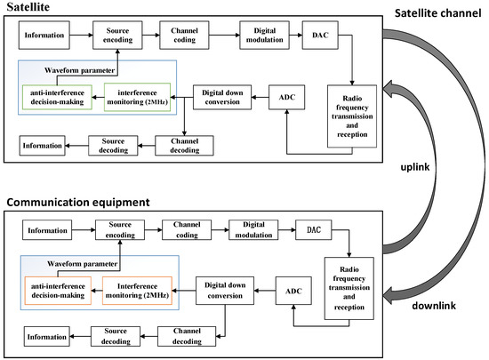
Figure 1.
Composition of anti-interference communication system.
The user monitors the downlink channel to perceive whether the satellite downlink data is interfered, and selects appropriate anti-interference waveform parameters through anti-interference decision-making technology. The waveform parameters are transmitted to the satellite through the uplink, based on which, the satellite adjusts the waveform to equip itself with the ability of anti-interference, thereby improving the communication quality and reliability of the downlink. Similarly, the satellite monitors the uplink channel and transmits the anti-interference waveform parameters to the user through downlink in the same way, so as to improve the user’s transmission waveform and improve the communication quality and reliability of the uplink.
To sum up, the anti-interference communication system between users and satellites can sense the characteristics of the space electromagnetic spectrum, search idle channels, identify enemy interference modes, and reconstruct the anti-interference communication link between users and satellites, so as to improve the reliability of emergency search. Both user and satellite use anti-interference and anti-interception technology, which includes three parts: interference monitoring technology, anti-interference decision technology and waveform generation technology. The waveform of the user terminal is generated according to the anti-interference decision-making parameters of the satellite and the waveform of the satellite is generated according to the anti-interference decision-making parameters of the user.
3. Interference Monitoring Research
Interference monitoring technology is an important part of anti-interference technology in communication systems. The interference monitoring technology in this study needs to judge whether the interference signal exists, and give the information such as the type of interference, the bandwidth range of the interference, the interference intensity and the interference frequency. Interference monitoring provides a priori information for communication anti-interference technology. It is not only the premise and foundation of cognitive and intelligent anti-interference systems, but also one of the key technologies.
In order to study the interference in satellite communication systems, this study first analyzes and models the satellite communication channel, and then analyzes the style and mathematical model of existing man-made interference signals [19]. Aiming at the problem of interference monitoring, this paper studies the advantages and disadvantages of the existing artificial feature extraction methods, and finally puts forward the interference monitoring technology based on deep learning.
3.1. Interference Signal
Interference signal is a broad concept, which is usually the general name of various signals harmful to useful signals. Generally, interference signals can be simply divided into human interference and non-human interference. Non-human interference is mainly determined by the communication environment. It is relatively stable in a certain area and a certain period of time, and the power is small and easy to suppress, which will not be studied by this paper. Human interference has great randomness, and the interference power is greater than that of non-human interference. Additionally, the interference frequency band is more targeted, which has a serious impact on communication.
The influence of interference signals on communication is different, and the frequency characteristics and time characteristics of different interference signals may also be different. According to the relative size of the spectrum width of interference and the spectrum width of spread spectrum signal, the interference in satellite communication systems can be divided into narrowband interference and wide band interference. The narrowband interference mentioned here refers to the interference signal whose bandwidth is far less than that of the spread spectrum signal, including continuous wave interference and other possible narrowband digital interference. Broadband interference refers to those interference signals whose bandwidth is comparable to that of spread spectrum signals, including continuous wave interference, linear frequency modulation interference, pulse interference, broadband comb-spectrum interference, frequency hopping interference and other spread spectrum signals [20,21].
3.2. Interference Monitoring Technology Based on Artificial Feature Extraction
The general process of interference monitoring technology is shown in Figure 2, including interference signal existence check, interference signal classification and interference parameter estimation. Firstly, the technology detects the interference of the received sampling data to judge whether the interference signal exists [22,23]. When there are interference signals, the interference is classified and the parameters are estimated. Finally, the results of detection and recognition are output.
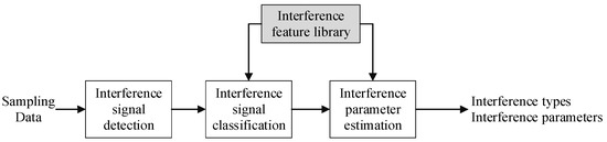
Figure 2.
Interference monitoring process.
3.2.1. Interference Signal Existence Check
Interference signal existence check is a typical binary hypothesis test problem, and its purpose is to judge whether the received signal contains interference. The interference detection algorithm mainly constructs a detection statistic with numerical difference between the presence and absence of interference signals, and judges the existence according to the statistic and given decision threshold.
Some typical detection statistics include carrier to noise ratio (CNR), sum of squares of CNR, average power, average value of each power spectrum, distribution difference of each frequency slice in the spectrum, ratio of maximum and secondary maximum eigenvalues of received signal correlation matrix, peak of cyclic spectrum, signal power ratio before and after interference suppression, peak frequency point power after median filtering, etc. [24,25].
The selection of decision threshold is mainly determined by the distribution of detection statistics and the detection performance requirements. However, the existing interference signal existence-checking algorithm can only judge whether there is interference in the received signal, and does not have the ability to estimate the interference position and interference parameters.
3.2.2. Interference Signal Classification
Interference signal classification (also known as interference detection or interference recognition) is actually a typical application of pattern recognition, which includes three steps: data pre-processing, feature extraction and classification.
The first is to pre-process the input data, that is, to preliminarily process the original signal data and map the signal from the signal space to the observation space. The process mainly includes: orthogonal down conversion, filtering, in-phase orthogonal decomposition, carrier estimation and carrier frequency component elimination. This step is to prepare for the feature extraction.
The second step is feature extraction. The purpose is to map the signal data of high-dimensional observation space to low-dimensional observation space, and extract the time domain characteristics, frequency domain characteristics, time frequency domain characteristics, transform domain characteristics and various statistical characteristics of the received signal. Selecting useful features is a very important step in the process of interference signal classification.
The third step is classification decision-making. The basic concept of classification decision-making is to classify the identified targets into certain categories through pattern recognition in feature space. Therefore, it is necessary to input the extracted feature parameters into the designed classifier, and then identify the corresponding signal categories. The process is divided into two steps: one is learning, which finds appropriate decision rules through known samples; The second is recognition, which uses the rule to design a classifier to realize the classification and recognition of unknown types of signals.
The data preprocessing is a relatively simple part, which will not be introduced here. And this paper focuses on feature extraction and classification decision-making.
3.2.3. Interference Parameters Estimation
The interference parameter estimation algorithm mainly analyzes the spectrum of the received signal to distinguish the interference frequency points from the non-interference frequency points. At present, some typical methods have been proposed to locate the frequency components of interference. These methods mainly include continuous mean elimination (CME) algorithm, forward continuous mean elimination (FCME) algorithm, FCME algorithm based on double threshold and FCME algorithm based on adjacent cluster merging (acc-fcme) [26]. With these methods, the frequency band, frequency bandwidth and Interference to noise ratio (Jnr) of interference can also be further estimated.
3.2.4. Advantages and Disadvantages
On the whole, there are many existing artificial interference features that can accurately reflect the physical characteristics of specific interference signals owing to long-term research on artificial feature extraction. The interference feature has clear mathematical definition and physical meaning. The structure of the classifier has good transparency and readability. Once there is an abnormal result, it is easy to locate quickly.
The disadvantage of the traditional artificial feature extraction method is that it requires manual selection of the appropriate feature parameters for specific interference types. When adding new interference, it needs to re-select the parameters and train the classifier. In addition, when there are many interference types, the process of manual feature selection will be very cumbersome and difficult to operate.
3.3. Interference Monitoring Technology Based on Deep Learning
In the face of multi type interference and complex scene, the traditional artificial feature extraction method is slightly weak. The interference monitoring technology based on deep learning can further improve the ability and effect of interference feature extraction, and solve the problem that the traditional artificial feature extraction lacks guidance on the selection and combination of multiple interference features due to the high data compression ratio of feature parameters. The deep learning method obtains the interference feature map or feature sequence through supervised learning, which enhances the representation of interference features at the expense of physical interpretability.
This section specifically introduces the interference monitoring technology based on deep learning proposed in this scheme, including method principle, network framework, data set construction, model training and experimental evaluation.
3.3.1. Overview of Method Principle
The deep learning method can predict the interference parameters, including the start and end time, start and end frequency, interference energy and bandwidth of the interference signal. The interference monitoring based on deep learning adopts the object detection method in image processing, inputs the time–frequency image of the signal, takes the interference signal as the detected target, and outputs the detection frame and prediction type of the interference signal. As shown in Figure 3, the image coordinates of the detection frame can be converted into the start and end time and start and end frequency corresponding to the interference signal according to the proportion. The brightness value of the interference signal in the detection frame and the width of the brightness area can be correspondingly converted into the energy and bandwidth information of the interference.
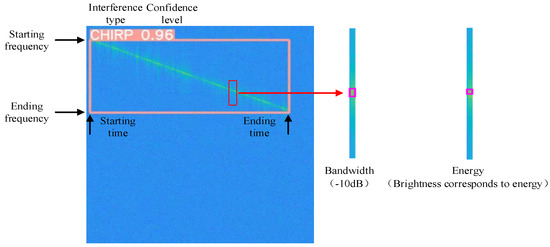
Figure 3.
Time frequency image interference monitoring results.
The time spectrum image of the input signal can be obtained by short-time Fourier transform (STFT). STFT Fourier transforms the signal by selecting a sliding window function, and then takes the square of the modulus of the transformed signal to obtain the energy distribution map in time and frequency domain, which is called spectrum. The short-time Fourier transform provides a general method for the analysis of non-stationary signals in the field of signal analysis. Through the window function, the spectrum analysis of the signal in any time period can be realized. The perfect combination of time domain analysis and frequency domain analysis of the signal is helpful to extract the time–domain characteristics and frequency domain characteristics of the signal at the same time.
Target detection technology based on deep learning has developed rapidly, and has exceeded the human level. In this scheme, the target detection algorithm is used to retrain the model through the self-made data set to make it have the ability to detect interference signals.
3.3.2. Network Structure
As shown in Figure 4, the network structure of this model is mainly composed of backbone network, neck network and head network. The backbone network mainly uses CSP (cross stage partial) darknet network and spatial pyramid pooling (SPP) structure, the neck network uses PANet structure, and the head network uses 1 × 1 Convolution
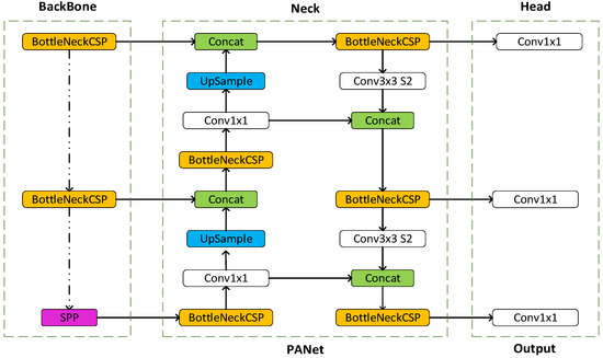
Figure 4.
Network structure.
The model uses CSP darknet as the backbone network to extract rich information features from the input image. CSP Net solves the problem of gradient information repetition in network optimization in other large convolutional neural network frameworks, and integrates the change of gradient into the feature graph from head to tail. Therefore, it reduces the amount of parameters of the model, which not only ensures the reasoning speed and accuracy, but also reduces the size of the model.
The neck network part of the model adopts PANet structure, and the neck network is mainly used to generate feature pyramid. The feature pyramid will enhance the detection of objects with different scaling scales, so that the same object with different sizes and scales can be recognized. PANet structure introduces bottom-up path augmentation structure on the basis of FPN. FPN mainly improves the effect of target detection by fusing high-level and low-level features, especially the detection effect of small-size targets. The bottom-up path enhancement structure can make full use of the shallow features of the network for segmentation. The network shallow feature information is very important for target detection, because target detection is a pixel level classification, and the shallow features are mostly edge shape and other features. PANet adds a bottom-up path enhancement structure on the basis of FPN, so that the top-level feature map can also share the rich location information provided by the bottom-level feature map, so as to improve the detection effect of large objects.
The head network of the model is a 1 × 1 convolution structure, and has three groups of output with different image feature rates. Finally, the anchor box will be applied to the output feature map, and the final output vector with category probability, confidence score and bounding box will be generated. On the anchor, the model distinguishes the positive and negative samples of the anchor by matching rules across the grid.
3.3.3. Dataset Construction
In the field of deep learning, the quality of data sets has a vital impact on solving problems. A high-quality dataset can often improve the quality of model training and the accuracy of prediction. Many researchers have spent a lot of effort on the creation and modification of data sets. However, in the practical application in specific fields, the public datasets play a limited role, and often cannot solve the problem with characteristics. The training effect on imagenet dataset with millions of samples may not be as good as the small dataset collected by researchers themselves. For the problem of interference information monitoring within 2 MHz monitoring bandwidth, it is very necessary to make a specific data set in this scheme.
An excellent dataset is composed of two characteristics: the distribution and diversity of the dataset is close to the real application scenario.
In order to ensure the diversity of data, this scheme makes diversified changes from three aspects: interference type, transformation range of interference frequency and interference duration. For the monitoring bandwidth of 2 MHz, the frequency conversion range of all interference signals designed in this scheme is 35 KHz to 1975 KHz. Since the time-frequency map is obtained from the sampled data per second through SIFT, the time corresponding to the abscissa of each time-frequency map is 1 s. In this scheme, the duration of all interference information is set in the range of 1 ms to 1000 ms.
The dataset is composed of four types of interference: single frequency interference, frequency hopping interference, frequency sweeping interference and unknown interference. Among them, there are two types of sweep interference: single sweep and round-trip sweep. In addition to normal single tone, single frequency interference also includes sweep frequency interference with small slope (aspect ratio greater than 20). As shown in Figure 5, the dataset has six types of interference patterns, which fully ensures the diversity of interference signals.
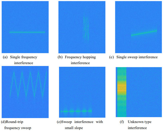
Figure 5.
Time frequency diagram of six kinds of interference. (a) Single frequently interference, (b) Frequency hopping interference, (c) Single sweep interference, (d) Round-trip frequency sweep, (e) Sweep interference, (f) Unknown type interference.
In addition, in order to make the data set close to the real scene, this scheme simulates and realizes three common channels: Gaussian channel, rice channel and Rayleigh channel according to the modeling of satellite communication channel in Section 3.1; Three different signal-to-noise ratios (SNR): 5 dB, 8 dB and 10 dB, are set to ensure the diversity of interference energy. Taking single tone interference as an example, Figure 6 shows the time–frequency diagram of single tone interference signal passing through three different channels under 10 dB signal-to-noise ratio; Figure 7 shows the time frequency diagram of single tone interference signal under three different drying ratios in Gaussian channel.
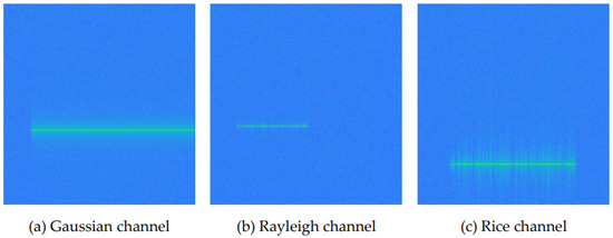
Figure 6.
Time frequency diagram of single frequency interference in different channels, SNR = 10 dB. (a) Gaussian channel, (b) Rayleigh channel, (c) Rice channel.
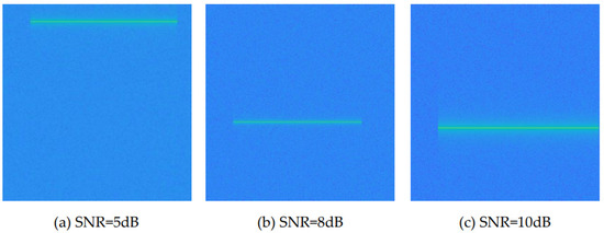
Figure 7.
Time frequency diagram of single frequency interference with different SNR in Gaussian channel. (a) SNR = 5 dB, (b) SNR = 8 dB, (c) SNR = 10 dB.
To sum up, the sample diversity of the data set can be expressed as follows:
- Interference type: single frequency, single sweep, round-trip sweep, small slope sweep, frequency hopping, unknown type interference
- Channel type: Gaussian white noise channel, Rayleigh channel, Rice channel
- Interference- noise ratio: 5 dB, 8 dB, 10 dB.
3.3.4. Model Training
The data is simulated by MATLAB, and the monitoring bandwidth is 2 MHz. The sampling data is stored in the format of binary bin file as the input of the model. The training set and test set data are divided by 10:1. There are 27,000 sample data in the training set and 2700 sample data in the test set.
Both the training set and the test set contain six kinds of interference patterns. Each group of data has 9 combination modes according to three channel types and three SNR. The training set consists of 500 samples × 9 species, a total of 4500 samples. Similarly, a set of data is tested by 50 samples × 9 species, a total of 450 samples.
The interference monitoring model uses self-made training set and test set to train the model parameters (Figure 8). Image size is 512 × 512 px, because the model needs 5 down samples, the length and width of the picture should be an integral multiple of 32. The number of iterations is set to 20, and 16 pictures are processed in batches each time. The learning rate is set to 0.01 and the weight attenuation rate is 0.0005.
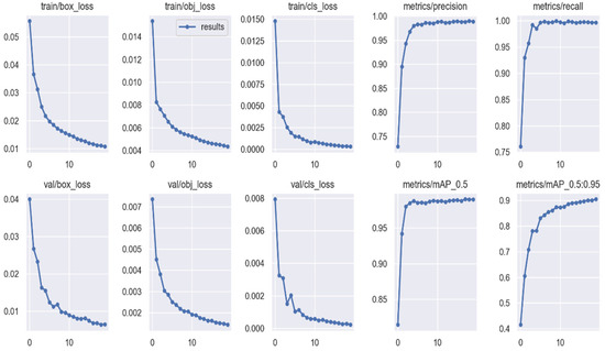
Figure 8.
Variation diagram of model loss function during training.
3.3.5. Experimental Evaluation
Evaluation Index
The Interference pattern evaluation index is demonstrated as follows:
The confusion matrix, accuracy and recall rate are proposed as evaluation indicators for interference patterns. The prediction accuracy of each type of interference and the recall rate of each type of interference are calculated to reflect the performance of the model. The classification results of all interference styles will be displayed in a confusion matrix to clearly show the relationship and distribution between the real value and predicted value of each type of interference.
Confusion matrix, also known as error matrix, is a standard format for accuracy evaluation, which is expressed in the form of matrix with n rows and N columns. In artificial intelligence, confusion matrix is a visual tool, especially for supervised learning. In the image accuracy evaluation, it is mainly used to compare the classification results with the actual measured values. The accuracy of the classification results can be displayed in a confusion matrix.
In the two classification model, the confusion matrix combines all the results of the predicted situation with the actual situation to form four situations: true positive, false positive, true negative and false negative, which are represented by , , and , respectively (T represents correct prediction and F represents wrong prediction).
Precision (P) also known as precision refers to the ratio of the number of correctly classified samples to the total number of classified samples. The formula is as follows:
Recall (R), also known as recall, shows the ratio of the number of correctly classified samples to the total number of samples that should be classified. The formula is as follows:
Here, the Interference parameter evaluation index is shown below.
The carrier position and interference start and end time in the interference parameters are analyzed quantitatively. The performance of the model prediction is characterized by calculating the root mean square error and average absolute error between the real value and the predicted value.
Root mean square error (RMSE) is used to measure the deviation between the observed value and the real value. The formula is as follows:
Mean absolute error (MAE) is the average of the absolute value of the deviation between all individual observations and the arithmetic mean. The average absolute error can avoid the problem of error cancellation, so it can accurately reflect the actual prediction error. The formula is as follows
where is the predicted value, is the real value, and N is the number of samples.
Model Performance Analysis
Some parameters are calculated to measure the model performance. The predicted value of the model is compared with the real value of the label. Accuracy and recall of the prediction are calculated, and the confusion matrix of interference pattern classification results are displayed. The root mean square error and average absolute error are also considered.
Figure 9 is a confusion matrix diagram of the classification results of four types of interference signals (single sweep and round-trip sweep are classified into the same category). It can be seen from the figure that the categories of interference signals are accurately predicted. Combined with Table 1, the accuracy and recall rate of interference signals are close to 100%.
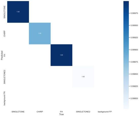
Figure 9.
Confusion matrix of interference pattern classification results.

Table 1.
Quantitative record of interference pattern test results.
Since the SIFT compresses the data, there is a quantization error of 2 ms in time and 4 KHz in frequency. Table 2 and Table 3 are the root mean square error and absolute error of interference signal prediction parameters respectively. Single frequency interference has only one carrier frequency. Since the frequency conversion range of small slope sweep interference is small, only its center frequency is predicted in this paper.
Table 2.
Root mean square error of interference identification parameter test.
Table 3.
Average absolute error of interference identification parameter test.
It can be seen from Table 2 that the root mean square error of predicting the start and end time of four types of interference signals is less than 4 ms. Among them, the end time prediction of sweep interference is the most accurate, and the root mean square error is 1.1 milliseconds. However the root mean square error of starting time prediction is the largest (3.7 ms). The root mean square error of the other three types is about 2 ms, which is basically caused by quantization.
In Table 2, the root mean square error of the start and end frequencies of the four types of interference information or the prediction of a single frequency point is less than 6 KHz. Among them, the prediction error of single tone interference frequency point is the smallest, followed by small slope sweep interference. The root mean square error of starting and ending frequency prediction of frequency hopping interference and frequency sweeping interference is large.
The results in Table 3 are consistent with the results in Table 2. The average absolute error of the end time of frequency sweeping interference is 2.2 ms and the average absolute error of the start and end time of other interference signals is less than 2 ms. In addition, the average absolute error of the prediction of the starting and ending frequency of the interference is the largest, followed by frequency hopping interference. The prediction error of single frequency interference and small slope sweep interference is the smallest. The average absolute error of the start and end frequency is less than 5 KHz.
3.3.6. Discussion
In the section, we present an external discussion. Firstly, the experiment proved that the algorithm has excellent detection effect, the accuracy and recall rate of 5 types of interference signals are nearly 100%, the prediction error is less than 4 ms and the prediction error is less than 6 KHz. Secondly, the monitoring bandwidth range reaches 2 MHz. In addition, the algorithm has successfully solved the detection problem of long duration monotone interference and small slope interference, making the detection accuracy and recall rate close to 100%.
4. Conclusions
The deep learning-based interference monitoring method proposed in this scheme outperforms other deep learning methods. Other deep learning methods typically only detect the interference styles, treating the problem as a classification problem. This method treats interference detection and parameter identification as target detection problems, and the main advantages are as follows:
At present, the interference signal detection and identification methods based on deep learning mainly aim at the interference signal detection and classification under the condition of single channel, but fail to realize the interference signal detection and classification under the condition of multi-channel broadband. At the same time, the existing research methods mainly identify the types of interference signals through correlation detection algorithms, which are not likely to identify the basic parameters such as the starting and ending frequency, energy and bandwidth of interference signals. Compared with the existing methods, the interference signal feature extraction and pattern classification algorithm based on deep learning proposed in this paper can complete the detection and classification of broadband interference signals and the parameter identification of interference signals.
In conclusion, the interference detection proposed in this scheme has excellent detection performance, high detection accuracy and small rate of error in parameter prediction, which can be used for communication satellite channel monitoring.
Author Contributions
Conceptualization, Y.Z. and J.Q.; methodology, J.Q.; software, J.Q.; validation, J.Q. and F.Z.; formal analysis, J.Q.; investigation, K.W. and J.Q.; resources, C.D.; data curation, J.Q., C.D. and J.Q.; writing—original draft preparation, J.Q.; writing—review and editing, J.Q. and Y.Z.; visualization, J.Q.; supervision, Y.Z.; project administration, Y.Z. All authors have read and agreed to the published version of the manuscript.
Funding
This research received no external funding.
Institutional Review Board Statement
Not applicable.
Informed Consent Statement
Not applicable.
Data Availability Statement
Not applicable.
Conflicts of Interest
The authors declare no conflict of interest.
References
- Shahid, S.M.; Teklay, S.Y.; Won, S.H.; Kwon, S. Load Balancing for 5G Integrated Satellite-Terrestrial Networks. IEEE Access 2020, 99, 1. [Google Scholar] [CrossRef]
- Jia, M.; Zhang, X.; Sun, J.Y. Intelligent Resource Management for Satellite and Terrestrial Spectrum Shared Networking toward B5G. IEEE Wirel. Commun. 2020, 27, 54–61. [Google Scholar] [CrossRef]
- Koroniotis, N.; Moustafa, N.; Slay, J. A new Intelligent Satellite Deep Learning Network Forensic framework for smart satellite networks. Comput. Electr. Eng. 2022, 99, 107745. [Google Scholar] [CrossRef]
- Petrovic, R.; Simic, D.; Cica, Z.; Drajic, D.; Nerandzic, M.; Nikolic, D. IoT OTH Maritime Surveillance Service over Satellite Network in Equatorial Environment: Analysis, Design and Deployment. Electronics 2021, 10, 2070. [Google Scholar] [CrossRef]
- Jiangyi, Q.; Wei, C. Coupling of an IOT wear sensor and numerical modelling in predicting wear evolution of a slurry pump. Powder Technol. 2022, 404, 117453. [Google Scholar]
- Li, G.; Wang, W.; Wu, Q.H. Cognitive Intelligent Spectrum Management and Control for Low-Earth-Orbit Satellite Systems. ZTE Technol. J. 2021, 27, 7–11. [Google Scholar]
- Lagunas, E.; Sharma, S.K.; Maleki, S.; Chatzinotas, S.; Ottersten, B. Resource allocation for cognitive satellite communications with incumbent terrestrial networks. IEEE Trans. Cogn. Commun. Netw. 2015, 1, 305–317. [Google Scholar] [CrossRef] [Green Version]
- Wu, Q.; Qiu, J.; Ding, G. Machine Learning Methods for Big Spectrum Data Processing. J. Data Acquis. Processing 2015, 30, 703–713. [Google Scholar]
- Zuo, Y.; Wu, Y.; Min, G.; Cui, L. Learning-based network path planning for traffic engineering. Future Gener. Comput. Syst. 2019, 92, 59–67. [Google Scholar] [CrossRef]
- Zuo, Y.; Wu, Y.; Min, G.; Huang, C.; Pei, K. An intelligent anomaly detection scheme for micro-services architectures with temporal and spatial data analysis. IEEE Trans. Cogn. Commun. Netw. 2020, 6, 548–561. [Google Scholar] [CrossRef]
- Rajendran, S.; Meert, W.; Giustiniano, D.; Lenders, V.; Pollin, S. Deep learning models for wireless signal classification with distributed low-cost spectrum sensors. IEEE Trans. Cogn. Commun. Netw. 2018, 4, 433–445. [Google Scholar] [CrossRef] [Green Version]
- Kim, B.; Kim, J.; Chae, H.; Yoon, D.; Choi, J.W. Deep neural network-based automatic modulation classification technique. In Proceedings of the 2016 International Conference on Information and Communication Technology Convergence (ICTC 2016), Jeju, Korea, 19–21 October 2016; pp. 579–582. [Google Scholar]
- Mendis, G.J.; Wei, J.; Madanayake, A. Deep learningbased automated modulation classification for cognitive radio. In Proceedings of the 2016 IEEE International Conference on Communication Systems (ICCS 2016), Shenzhen, China, 14–16 December 2016; pp. 1–6. [Google Scholar]
- Wang, F.; Wang, Y.; Chen, X. Graphic constellations and DBN based automatic modulation classification. In Proceedings of the 2017 IEEE 85th Vehicular Technology Conference (VTC Spring), Sydney, NSW, Australia, 4–7 June 2017; pp. 1–5. [Google Scholar]
- Wang, D.; Zhang, M.; Li, J.; Song, C.; Chen, X. Intelligent constellation diagram analyzer using convolutional neural network-based deep learning. Opt. Express 2017, 25, 17150–17166. [Google Scholar] [CrossRef] [PubMed]
- Liu, Z.; Li, L.; Xu, H.; Li, H. A method for recognition and classification for hybrid signals based on deep convolutional neural network. In Proceedings of the 2018 International Conference on Electronics Technology (ICET 2018), Chengdu, China, 23–27 May 2018; pp. 325–330. [Google Scholar]
- Ren, J.; Zhang, X.; Xin, Y. Using Deep Convolutional Neural Network to Recognize LTE Uplink Interference. In Proceedings of the 2019 IEEE Wireless Communications and Networking Conference (WCNC), Marrakesh, Morocco, 15–29 April 2019; pp. 1–6. [Google Scholar]
- Daldal, N.; Cömert, Z.; Polat, K. Automatic determination of digital modulation types with different noises using convolutional neural network based on time–frequency information. Appl. Soft Comput. 2020, 86, 105834. [Google Scholar] [CrossRef]
- Chang, H.; Zhao, X.; Shi, H. Joint FFT spectrum energy and correlation detection based fast spectrum sensing method and performance analysis. Syst. Eng. Electron. 2021, 43, 1406–1412. [Google Scholar]
- Quyen, N.X.; Duong, T.Q.; Vo, N.S.; Xie, Q.; Shu, L. Chaotic direct-sequence spread-spectrum with variable symbol period: A technique for enhancing physical layer security. Comput. Netw. 2016, 109, 4–12. [Google Scholar] [CrossRef]
- Fu, Y.; Guo, S.; Yu, Z. The modulation technology of chaotic multi-tone and its application in covert communication system. IEEE Access 2019, 7, 122289–122301. [Google Scholar] [CrossRef]
- Block, D.; Töws, D.; Meier, U. Implementation of efficient real-time industrial wireless interference identification algorithms with fuzzified neural networks. In Proceedings of the 2016 24th European Signal Processing Conference (EUSIPCO), Budapest, Hungary, 29 August–2 September 2016; pp. 1738–1742. [Google Scholar]
- Grimaldi, S.; Mahmood, A.; Gidlund, M. Real-Time Interference Identification via Supervised Learning: Embedding Coexistence Awareness in Io T Devices. IEEE Access 2019, 7, 835–850. [Google Scholar] [CrossRef]
- Jiang, G.; Sun, C.; Liu, X.; Li, M.; Jiang, G. Power spectral density estimation of ship-radiated noise based on multipath channel. J. Appl. Acoust. 2020, 39, 81–88. [Google Scholar]
- Chen, Y.; Wei, S.; Zhang, Y. Classification of heart sounds based on the combination of the modified frequency wavelet transform and convolutional neural network. Med. Biol. Eng. Comput. 2020, 58, 2039–2047. [Google Scholar] [CrossRef] [PubMed]
- Yu, G.; Wang, H.; Du, W. Cooperative Spectrum Sensing Algorithm to Overcome Noise Fluctuations Based on Energy Detection in Sensing Systems. Wirel. Commun. Mob. Comput. 2021, 2021, 5516540. [Google Scholar] [CrossRef]
Publisher’s Note: MDPI stays neutral with regard to jurisdictional claims in published maps and institutional affiliations. |
© 2022 by the authors. Licensee MDPI, Basel, Switzerland. This article is an open access article distributed under the terms and conditions of the Creative Commons Attribution (CC BY) license (https://creativecommons.org/licenses/by/4.0/).