A DASKL Descriptor via Encoding the Information of Keypoints and a 3D Local Surface for 3D Matching

Abstract

Three-dimensional matching is widely used in 3D vision tasks, such as 3D reconstruction, target recognition, and 3D model retrieval. The description of local features is the fundamental task of 3D matching; however, the descriptors only encode the surrounding surfaces of keypoints, and thus they cannot distinguish between similar local surfaces of objects. Therefore, we propose a novel local feature descriptor called deviation angle statistics of keypoints from local points and adjacent keypoints (DASKL). To encode a local surface fully, we first calculate a multiscale local reference axis (LRA); second, a local consistent strategy is used to redirect the normal direction, and the Poisson-disk sampling strategy is used to eliminate the redundancy in the data. Finally, the local surface is subdivided by two kinds of spatial features, and the histogram of the deviation angle between the LRA and the normal point in each subdivision space is generated. For the coding between keypoints, we calculate the LRA deviation angle between the nearest three keypoints and the adjacent keypoint. The performance of our DASKL descriptor is evaluated on several datasets (i.e., B3R, UWAOR, and LIDAR) with respect to Gaussian noise, varying mesh resolutions, clutter, and occlusion. The results show that our DASKL descriptor has achieved excellent performance in terms of description, robustness, and efficiency. Moreover, we further evaluate the generalization ability of the DASKL descriptor in a LIDAR real-scene dataset.

1. Introduction

In recent years, with the flourishing of low-cost sensors, such as Microsoft Kinect, Google Project Tango, and Intel RealSense, as well as high-speed computing systems, 3D data can be easily obtained, and the 3D computer vision area has been widely used in robots [1], reverse engineering [2], autopilot [3] and biometric systems [4,5], and other fields. In these aforementioned 3D applications, the description of local features is a fundamental and crucial step. With the advancement of descriptors, a variety of techniques have been used to construct local feature descriptors, mainly based on manual design and deep learning. The research on methods based on deep learning is mainly focused on the representation of point cloud inputs, taking the local feature descriptor of point clouds as an input or regularizing direct point clouds, after which a network structure is designed for the inputs (i.e., ClusterNet [6], SpinNet [7], RPM-Net [8], and PR-InvNet [9]). Although it has developed rapidly, it is limited by the deficiency of large point cloud datasets for specific tasks, computer resources, which are very costly, and edge devices that still may not be equipped with GPUs. Therefore, in current practical applications, methods based on manual design still play an important role; they are mainly constructed through the statistics of spatial and geometric properties or the representation of the relationship between points. For details on the existing local feature descriptors, readers can refer to a recent survey [10].

The research scope of this paper focuses on the local feature description of manual design. A local feature descriptor with good performance should have high descriptiveness and strong robustness, as well as efficient time performance [11]. Descriptiveness represents a descriptor’s ability to distinguish between different surfaces, while robustness shows a descriptor’s ability to resist disturbances, including noise, varying resolutions, and occlusion; for the invariance of translation, scaling, and rotation, the time performance requires the computational efficiency of the descriptor [12]. In the past two decades, many local feature descriptors have been designed, including FPFH [13], SHOT [14], and ROPS [15]; the local frame and feature coding are the two main parts that determine their performance. The local frame is a local axis or coordinate system used to align with a local surface, enabling the rigid transformation invariance of local feature descriptors. Additionally, feature coding means converting the geometrical and spatial information of a local surface into a feature vector representation.

Local frames can be divided into a local reference frame (LRF) and a local reference axis (LRA). The LRF consists of three axes, while the LRA consists of the z-axis. The repeatability of the x-axis and y-axis of the LRF is more easily affected by various disturbances (for example, noise, varying resolutions, and symmetric surfaces) than the z-axis, and more time is required to construct it than is required for the LRA [16]. The literature [16] combines the method based on the LRA and the method based on the LRF with different coding methods, and performs a large number of comparative experiments to prove that the method based on the LRA, combined with radial information and elevation information, has stronger robustness against all kinds of interferences. For LRA-based descriptors, the repeatability of the LRA directly affects the performance of these descriptors. In order to achieve the high repeatability of local reference frames, many methods have been proposed to construct LRF/As; among these methods, the LRA usually uses covariance analysis techniques in its construction, which represent the LRA as a standardized eigenvector corresponding to the minimum eigenvalue of the covariance matrix [17]. These methods have the problem of symbol ambiguity, for which Tombari et al. [1] proposed a disambiguation technique. In addition, they introduced an LRA based on a linearly weighted covariance matrix, it is robust against noise but its vulnerability to varying data resolutions. Guo et al. [15] proposed a new method to construct an LRA that needed to calculate the covariance matrix of each triangular mesh in the local neighborhood, so its efficiency was not high. Yang et al. [17] used a subset of the radius neighborhood to construct a covariance matrix, which improved its robustness against occlusion, clutter, and mesh boundaries. Zhao et al. [12] improved the LRA proposed by Yang, using a subset of radius neighborhoods to calculate directions and using all of the radius neighborhoods to eliminate symbolic ambiguity; although it reduces the robustness against grid boundaries, it improves the robustness against noise and varying resolutions. Therefore, the performance of the LRA calculated by different neighborhood scales was different, and the robustness against multiple disturbances cannot be obtained at the same time.

In a feature representation of a feature descriptor, the geometric information and spatial information of a local surface are usually encoded. Some existing descriptors only encode the geometric information of a local surface, and the angle of deviation between normals or LRAs and normals is an effective way to encode local geometric information; for example, Rusu et al. [18] have proposed point characteristic histograms (PFHs) based on the relationship between points, their k-neighbors, and their estimated normals, which are relatively robust but computationally inefficient. In order to improve the efficiency, they simplified the features and constructed a fast point feature histogram (FPFH) [13], which has a similar performance to the PFH and a higher efficiency, but only descriptors encoding geometric information usually show a poor performance in resisting noise, varying resolutions, etc. [10]. In contrast, some descriptors encode only spatial information on a local surface. Johnson et al. proposed the spin image feature (SI) [19], which uses normals as its LRA, after which each point within the support area is represented by two spatial distances, and, finally, the SI is generated by calculating the distribution of local points along both the spatial measures. The SI completely encodes local spatial information on an LRA but is sensitive to noise due to the low repeatability of its LRA [10]. Tombari et al. [20] proposed a unique shape context (USC) developed from a 3D shape context (3dsc) descriptor [21]. The USC completely encodes the spatial information on the LRF by compartmentalizing it locally in a 3D spatial manner along the orientation, elevation, and radial directions, showing great robustness against noise, hetero waves, and occlusion, but showing sensitivity to variations in data resolution [10]. There are also some descriptors that encode both geometric and spatial information, and Tombari et al. [14] proposed an LRF-based direction histogram (SHOT) descriptor signature method, which is highly descriptive but very sensitive to variations in grid resolution. Some other local feature descriptors encode projection information based on different orientations of the LRF, which acquires redundant information (e.g., ROPS [15] and TOLDI [22]). Regardless of how to encode local information, due to the existence of symmetric objects or similar surfaces, encoding only local information will inevitably suffer from ambiguity, which in practical three-dimensional matching introduces a large number of false positives. Shah et al. [23] proposed KSR encoded only between keypoints, independent of local surfaces, and realized three-dimensional modeling and recognition, demonstrating that information encoding between keypoints is also an effective way of expressing features, but is sensitive to occlusion comparisons with solely keypoint information.

For these concerns, we propose a novel local feature descriptor named deviation angle statistics of keypoints from local points and adjacent keypoints (DASKL). Specifically, we first calculated the LRA of different scales of keypoints and the normals of neighbor points; when calculating the LRA, we adopted a multiscale calculation strategy, and the appropriate LRA was selected according to the scale strategy in the matching stage, which made the LRA more robust against noise, varying resolutions, and boundary grids at the same time. When calculating the normals, Poisson-disk sampling was carried out on the local surfaces to remove redundant points and reduce the amount of calculation. Second, the geometric and spatial information of local spaces were encoded based on the LRA. Based on the local neighborhood of the keypoints subdivided by the LRA, the deviation angle between the normal of neighborhood points in each partition and the LRA was counted. The geometric information between keypoints was encoded; we calculated the distance between the keypoints of the local feature descriptor, obtained the two nearest neighbor keypoints of each keypoint, and then counted the deviation angle of the LRA between the keypoints. Finally, the statistical coding information was connected in the form of a histogram to generate the DASKL descriptor. The main contributions of this paper are summarized as follows:

(1)

By encoding geometric information in subdivision spaces and combining the geometric information of keypoints and the last three keypoints, we propose the DASKL descriptor, which is highly descriptive and robust against occlusion, noise, and varying resolutions.

(2)

The DASKL descriptor fully encodes the spatial and geometric information of local surfaces in addition to combining the geometric information of keypoints and adjacent keypoints, which improves the ability of the local feature descriptor to distinguish between similar surfaces.

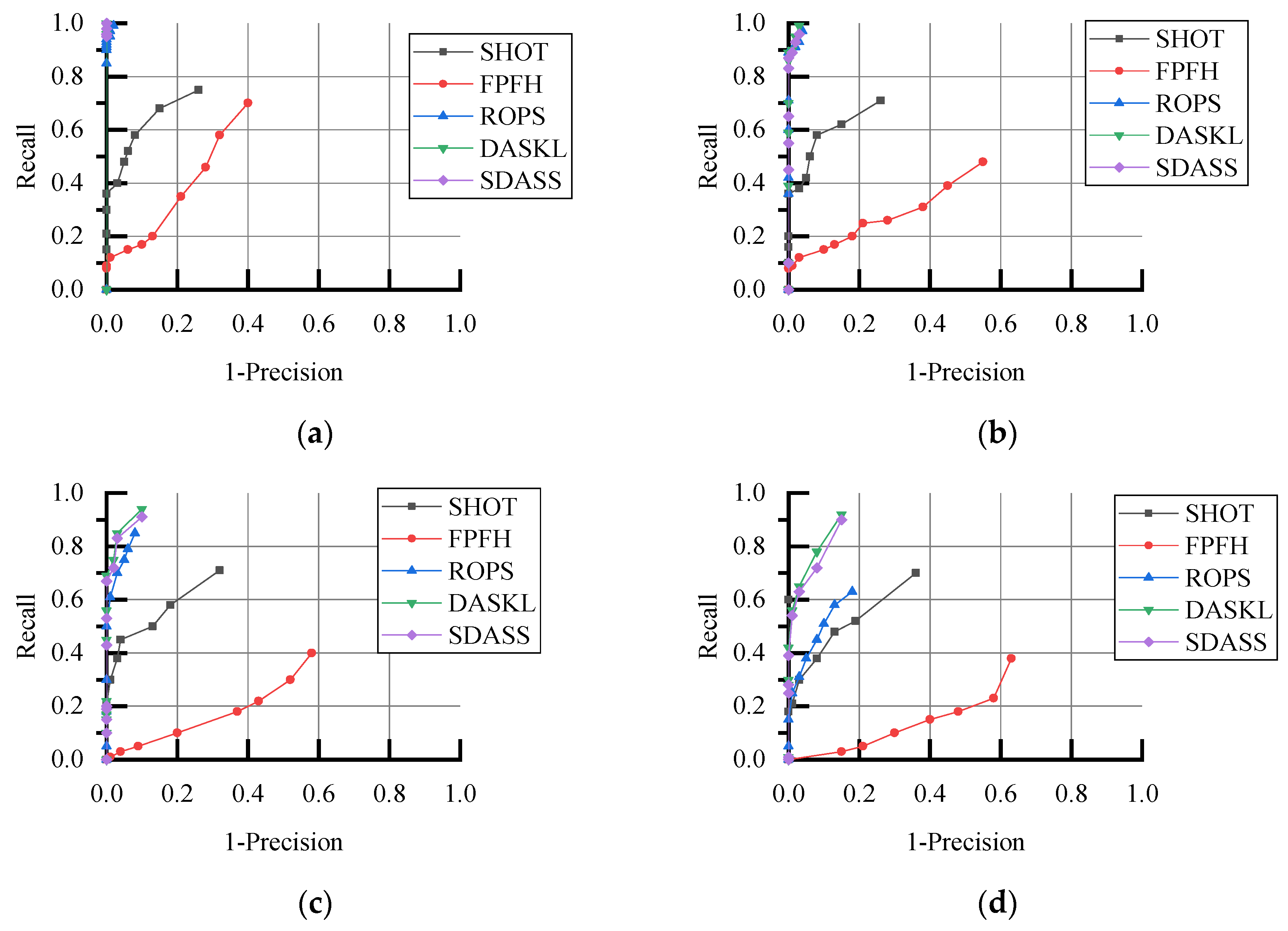
The rest of this paper is organized as follows: Section 2 describes the process of generating the DASKL descriptor in detail. Section 3 presents the evaluation results of our approach for two public datasets and a LIDAR real-scene dataset. Finally, conclusions and future work are provided in Section 4.

2. DASKL Local Feature Description

This section introduces some techniques involved in the DASKL descriptor in detail, including the construction of the LRA, the calculation of the normals, the coding between the keypoints and nearest neighbor keypoints, and the coding of the keypoints and local points, that is, to represent DASKL features by encoding the combination of the spatial and geometric information on the surface of an object.

2.1. Constructing the LRA

Our method chooses the LRA as the basis for space division at keypoints. Given a keypoint, p, and a support radius, R, all of the points in the radius range of the sphere are defined as neighborhood points of p points. These neighborhood points form a local surface:$Q=\left\{q_1,q_2,q_3,\dots \dots ,q_n\right\}$.

First, a subset of Q is defined as $Q_z=\left\{q_1^z,q_2^z,q_3^z,\dots \dots ,q_n^z\right\}$; to calculate the direction of the z-axis, the covariance matrix $\mathrm{Cov}\left(Q_z\right)$, based on $Q_z$, is defined as:

$$\mathrm{Cov}\left(Q_z\right)={\left[\begin{array}{c}{q}_1^z-\overline{q^z}\\ \dots \\ q_n^z-\overline{q^z}\end{array}\right]}^T\left[\begin{array}{c}{q}_1^z-\overline{q^z}\\ \dots \\ q_n^z-\overline{q^z}\end{array}\right],$$

(1)

where n is the size of $Q_z$, $\overline{q_z}$ is the center of gravity of $q_z$, and the eigenvector, $v\left(p\right)$, corresponding to the smallest eigenvalue of $\mathrm{Cov}\left(Q_z\right)$, is set to the z-axis. However, the direction of the eigenvector is random. In order to eliminate the ambiguity of $v\left(p\right)$, the LRA is generated by using the computational domain $R_s$:

$$\mathrm{LRA}\left(p\right)=\{\begin{array}{c}v\left(p\right),if v\left(p\right)·{\sum }_{i=1}^{n}p{q}_i\ge 0,\\ -v\left(p\right),others\end{array},$$

(2)

where n is the number of points in the computing field, $p{q}_i$ is the vector from $p$ to $q_i$, and the “·” between the vectors represents the dot product. The scope of the subset of $Q_z$ is defined as the computing domain $R_s:$

$$R_s =\mathsf{\lambda }\mathrm{R},$$

(3)

$\mathsf{\lambda }$ is a scale factor for adjusting the size of the computing domain. It is proven in [22] that the computational domain, $R_s$, used to estimate the z-axis is smaller than the supporting radius, R, which can improve the robustness of the LRA against clutter and occlusion, but it performs poorly in downsampled data. In [12], all of the radius neighborhoods are used to determine the direction of the LRA, and high robustness of varying data resolutions against noise and variation is obtained, but it is less robust against grid boundaries. Therefore, the selection of different scales affects the performance of the LRA. How to determine the appropriate calculation radius is a challenging task.

For the neighborhood subsets of the same scale of different data, the number of neighborhood points involved in calculating the z-axis is also different; for example, when LIDAR collects scenes’ data with long distances, the point clouds obtained are relatively sparse, that is, within the same radius the number of points in the scene is much smaller than that of the model, which is essentially related to the average data resolution of the point clouds. This is also reflected in the calculation of the LRF in [14,18]. The scene is consistent with the radius of the z-axis calculated by the model. On this basis, the scale factor, λ, is introduced to adjust the model and scene to improve the robustness against varying resolutions [24]:

$$\mathsf{\lambda }=\frac{s.mr}{c\times m.mr},$$

(4)

m.mr and s.mr are the average data resolutions of the model and the scene, respectively, and c is constant. Based on the experience of previous methods, we think that when the average resolution of the scene and the model is about the same, λ takes 3 as the best parameter, and R is the upper limit of the threshold. It should be emphasized that when the model descriptor is generated in the offline phase, the scene resolution is unknown. Therefore, the indexing strategy proposed in reference [24] is introduced to calculate the model descriptor of multiscale λ, and the model descriptor closest to λ, calculated by Formula (4), is selected in matching; thus, a nonfuzzy local reference frame LRA that is robust against scene interference is obtained.

2.2. Normal Calculation

At present, the common method of generating normals is to use principal component analysis (PCA) on the covariance matrix to calculate the normal of each point. The principal component analysis is based on the k-nearest neighbors of each point to create the covariance matrix. However, the normal direction calculated by PCA is not clear and is time-consuming. The local corresponding method in [25,26] is used to reorient the normal of each surface, such that the point is consistent with the direction of most normals in its radius neighborhood. For each point, pairi, and its original normal, nimi, as well as the k-nearest neighbors, $\left\{p_{i1},p_{i2},p_{i3},\dots ,p_{ik}\right\}$, calculate c_(pometi), that is, the centroid of the pairi neighborhood, as follows:

$$c_{p_i}=\frac{1}{k}{\sum }_{n=1}^k{p}_{in},$$

(5)

Next, define the normal after the ambiguity is eliminated:

$$n_i=\{\begin{array}{c}{n}_i, n_i·\left(c_{p_i}-p_i\right)\le 0\\ -n_i, n_i·\left(c_{p_i}-p_i\right)>0\end{array},$$

(6)

Using the above method, it is not possible to uniformly orient normals across the entire object, but this does not affect performance because it ensures that the normal directions of the corresponding points in the model and the scene are consistent, which improves the robustness of normal-based descriptors.

The adjacent points on the local surface have similar characteristics, which leads to a certain degree of information redundancy; therefore, as shown in [26,27], the Poisson-disk sampling algorithm is used to sample the model to retain the necessary description information and simplify the model.

2.3. Descriptor Generation

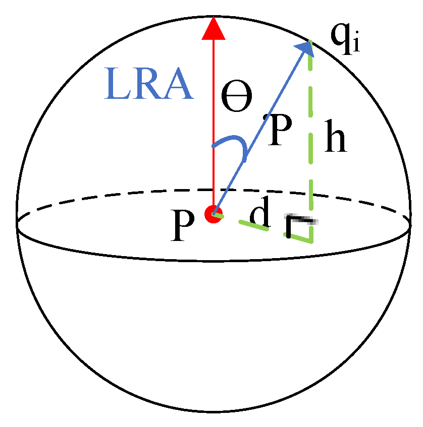
After constructing the LRA and normals, the spatial and geometric information are encoded on the local surface, and the geometric information of the keypoints and the three nearest keypoints are counted. In general, the spatial information of the local surface can be fully encoded on the LRA in two ways. It is verified by different spatial information methods in reference [1] that using projection radial distance and height distance to comprehensively encode the local spatial information of the LRA has the best performance. As shown in Figure 1, one method uses radial distance (ρ) and elevation (θ), and the other uses height distance (h) and projection radial distance (d). In this paper, projection radial distance and height distance are used to comprehensively encode the local spatial information of the LRA.

The local surface is determined by the feature point, p, and the support radius, R, and the local point cloud is defined as ${\mathrm{Q}=\{\mathrm{q}}_1{,\mathrm{q}}_2{, \dots ,\mathrm{q}}_{\mathrm{k}}\}$, as shown in Figure 2a. First, Q is transformed so that p coincides with the coordinate origin, and the LRA of the feature point is aligned with the z-axis, as shown in Figure 2b. Then, as shown in Figure 2c, the spatial information of the transformed local space is encoded. The spatial information coding method is to segment the local space along the LRA and the projection radial direction; ${\mathrm{N}}_{\mathrm{lh}}$ and ${\mathrm{N}}_{\mathrm{pr}}$ are the number of partitions along the LRA and the projection radial direction, respectively, and ${\mathrm{N}}_{\mathrm{ld}}$ is the number of partitions used to count the deviation angle. The division ranges of the LRA and projection radial direction are [0, 2r] and [0, r], respectively. After the partition of the local space is completed, the geometric information is encoded into each partition, as shown in Figure 2d.

In each partition, the geometric information is encoded using the statistics of the deviation angle between the feature point LRA and the normal of the adjacent points. The deviation angle between the normal and the LRA is calculated as follows:

$${\mathrm{nd}}_{\mathrm{i}}{(\mathrm{q}}_{\mathrm{k}})=\arccos (\mathrm{LRA}\left({\mathrm{p}}_{\mathrm{i}}\right){,\mathrm{n}}_{\mathrm{i}}{(\mathrm{q}}_{\mathrm{k}}\left)\right),$$

(7)

where LRA(p) represents the LRA; ${\mathrm{n}}_{\mathrm{i}}$ at the feature point, p, represents the normal at the local point, $q_k$; ${\mathrm{nd}}_{\mathrm{i}}$ represents the declination between the LRA (p) and n; and the range of ${\mathrm{nd}}_{\mathrm{i}}$ is [0,$\mathsf{\pi }$]. Encode the geometric information into a partition to generate a subhistogram of the statistical offset angle in that partition, called ${\mathrm{h}}_{\mathrm{i}}$. As shown in Figure 2e, after generating the subhistograms of all of the partitions, join all of the subhistograms into a single representation as ${\mathrm{H}=\{\mathrm{h}}_1{,\mathrm{h}}_2{, \dots ,\mathrm{h}}_{\mathrm{Nlh}*\mathrm{Npr}}\}$; the length of H is ${\mathrm{N}}_{\mathrm{lh}}{\times \mathrm{N}}_{\mathrm{pr}}{\times \mathrm{N}}_{\mathrm{ld}}$.

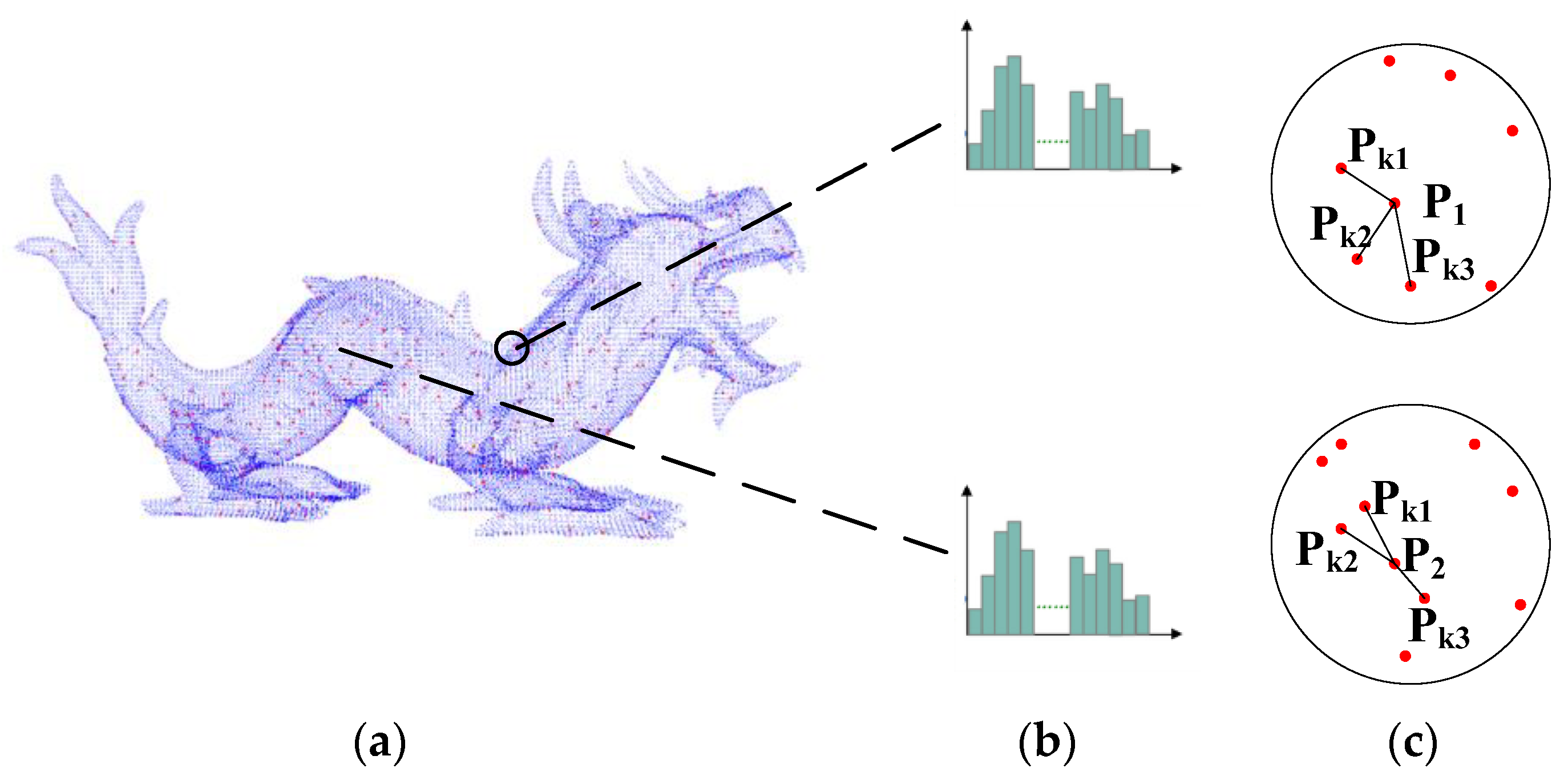
After coding the local surface of the feature points, as shown in (f) in Figure 2, the geometric information of p and the three nearest keypoints is counted. This step can be synchronized with the local features framed by dotted lines in Figure 2 to reduce the time overhead. Specifically, for the information coding between the keypoints, as shown in Figure 3a, the local surface information of the model “dragon” is taken as an example. First of all, if we only calculate the local surface features of the model “dragon”, we will obtain several similar descriptors, such as Figure 3b, which will lead to mismatching. However, as shown in Figure 3c for the surface similar keypoints, ${\mathrm{P}}_1$ and ${\mathrm{P}}_2$, the adjacent keypoints are ${\mathrm{P}}_{\mathrm{kn}}$, n = 1, 2, 3; ${\mathrm{P}}_1$ and ${\mathrm{P}}_2$ are different from the recent three keypoints, which increases the differentiation of their similar surfaces.

The following equation is used to calculate the distance between keypoints and other keypoints:

$$\mathrm{d}\left({\mathrm{P}}_{\mathrm{i}}{,\mathrm{P}}_{\mathrm{kn}}\right)=\sqrt{{\left({\mathrm{P}}_{\mathrm{i}}{-\mathrm{P}}_{\mathrm{kn}}\right)}^2},{\mathrm{P}}_{\mathrm{kn}}\in {\mathrm{R}}_{\mathrm{f}},$$

(8)

In order to improve the search efficiency, this paper sets the search radius, ${\mathrm{R}}_{\mathrm{f}}$, retrieves the nearest keypoints in the spherical domain within the search radius, and gradually expands the range of ${\mathrm{R}}_{\mathrm{f}}$ until the three nearest keypoints, ${\mathrm{P}}_{\mathrm{k}1}$, ${\mathrm{P}}_{\mathrm{k}2}$, and ${\mathrm{P}}_{\mathrm{k}3}$, are found.

After the three nearest keypoints are obtained, in order to further strengthen the differentiation between the keypoints, the deviation angle between the LRA at the keypoints is calculated to represent the geometric relationship between the keypoints. For a given feature point, (${\mathrm{P}}_{\mathrm{i}}$), the angle of deviation between its LRA is:

$${\mathrm{ld}(\mathrm{P}}_{\mathrm{i}}{, \mathrm{P}}_{\mathrm{k}}{)=\cos }^{-1}{(\mathrm{P}}_{\mathrm{i}}{, \mathrm{P}}_{\mathrm{k}}),$$

(9)

where ${\mathrm{ld}(\mathrm{P}}_{\mathrm{i}}{, \mathrm{P}}_{\mathrm{k}})$ indicates the deviation angle between the keypoints, and the range of the deviation angle is [0, π]. Finally, the information between the above keypoints is counted as a histogram, which is called ${\mathrm{H}}_{\mathrm{kp}}$, and the dimension is ${\mathrm{N}}_{\mathrm{kp}}$. The final length of the entire descriptor is ${\mathrm{N}}_{\mathrm{lh}}{\times \mathrm{N}}_{\mathrm{pr}}{\times \mathrm{N}}_{\mathrm{ld}}$+${\mathrm{N}}_{\mathrm{kp}}$; in order to achieve robustness against point cloud resolution, the whole descriptor is normalized to 1.

3. Experiments

In this section, we briefly introduce the Bologna 3D Retrieval (B3R) dataset [28,29], the UWAOR dataset [1,30], and a real-scene dataset, in addition to the evaluation criteria used in the experiments. The performance of the DASKL descriptor is also compared with several state-of-the-art methods (SDASS [12], FPFH [13], SHOT [14], and ROPS [15]) for rigorous evaluation. All of the experiments in this chapter were performed on computers equipped with an Intel Xeon Gold 6226R and 24 GB of RAM.

3.1. Datasets

3.1.1. B3R Dataset

The B3R dataset is a popular dataset in the field that is used to test 3D vision algorithms, such as feature description, recognition, registration, and so on. The B3R dataset consists of six different target types and 45 scenes, each of which consists of 3–5 randomly rotated and translated targets. All of the models come from the Stanford Repository, including the six models of Bunny, Dragon, Happy Buddha, Armdillo, ThaiStatue, and AsianDragon, as shown in Figure 4. In this paper, we will test the performance of the descriptor in different scene types (such as no noise, 0.1 mr Gaussian noise, 0.3 mr Gaussian noise, 0.5 mr Gaussian noise, 1/2 downsampling, 1/4 downsampling, and 1/8 downsampling).

3.1.2. UWAOR Dataset

The UWAOR (UWA Object Recognition) dataset is used to test the performance of local feature descriptors under occlusion. The UWAOR dataset consists of 5 object models with complete viewpoints and 50 scenes with specific viewpoints. Each scene is generated by placing four or five objects together randomly; for each object in the scene, the ground truth pose is a 4 × 4 transformation matrix. The total number of scene instances in the dataset is 188 (50 chef objects, 48 chicken objects, 45 Parasaurolophus objects, and 45 T-rex objects). The sample scene and objects are shown in Figure 5.

3.1.3. LIDAR Real Dataset

The LIDAR real dataset is used to test the matching performance of the DASKL descriptor in real complex environments. We use the RS-LiDAR-M1 LIDAR to gather data from different angles and distances. The dataset collects ground scenes containing 3 kinds of rigid targets, including 3 models and 25 complex ground scenes, which are a cannon, a tank missile vehicle, and a transport vehicle, respectively. Each scene is composed of a target model, the surrounding environment, including a variety of different targets, and the scene. Examples of a scene and object are shown in Figure 6.

3.2. Evaluation Criteria and Comparison Methods

The precision–recall curve (PRC) is a popular method for evaluating the matching performance of feature descriptors. We compare our method with several typical descriptors, including FPFH, SHOT, and ROPS, to evaluate performance under interference, including noise, different data resolutions, and occlusion. In the experiment of this paper, first, the logarithm of the corresponding keypoints is extracted according to the ground truth information of the dataset, after which uniform sampling is used to extract the keypoints of the scene and the model, and then the model features and scene features are calculated based on these keypoints. Finally, the total matching point pairs are obtained by feature matching, and the correct matching points are obtained by using the NNSR matching method [31] to set the threshold.

The 1-precision of feature descriptor matching is defined as the ratio of the mismatched logarithm to the total matching logarithm, as the horizontal axis:

$$1-\mathrm{precision}=\frac{\mathrm{No}:\mathrm{of} \mathrm{false} \mathrm{matches}}{\mathrm{No}:\mathrm{of} \mathrm{matches}},$$

(10)

The recall rate is defined as the ratio of the correct feature matching logarithm to the corresponding feature matching logarithm, as the vertical axis:

$$\mathrm{recall}=\frac{\mathrm{No}:\mathrm{of} \mathrm{false} \mathrm{matches}}{\mathrm{No}:\mathrm{of} \mathrm{corresponding} \mathrm{features}},$$

(11)

By changing the matching threshold, the Recallvs1–Precision curve is obtained. For a good feature descriptor, the PRC curve should be concentrated in the upper-left corner of the graph, that is, the feature descriptor has high recall and accuracy at the same time.

3.3. Performance Evaluation of DASKL

3.3.1. Matching Performance on Different Noise Levels

The scene of the B3R database contains different levels of Gaussian noise, and the standard deviation distribution is {0.1, 0.3, 0.5} pr. Eighteen scenes with different noise levels were randomly selected to match the model, and the PRC results are shown in Figure 7. From the point of view of robustness against noise, looking at Figure 7, we can see that DASKL still maintains high performance with the increase of noise level, followed by SDASS. In the experiments without noise, 0.1 pr and 0.3 pr, ROPS maintains a performance similar to DASKL, but when adding 0.5 pr of noise the performance decreases. With the improvement of the noise level, SHOT maintains a stable performance, but there is an obvious gap between DASKL and SDASS. FPFH is very sensitive to noise, and the performance decreases significantly after increasing noise, mainly because it only uses normals to extract geometric information. The influence of noise on the spatial distribution of point clouds is small, but it changes obviously on the geometric properties of point clouds, so the robustness against noise of DASKL, ROPS, and SHOT using spatial distribution information is higher than that of FPFH, which only extracts geometric information.

3.3.2. Matching Performance on Different Downsampling Levels

Eighteen scenes with different downsampling levels were randomly selected to match the model, and the downsampling levels were 1/2, 1/4, and 1/8, respectively, and the PRC image is shown in Figure 8. The performance of each descriptor has different degrees of performance degradation as the downsampling level increases, and the performance gap becomes more and more obvious because when the point cloud is too sparse the geometric edges of the object are not obvious and the number of points in the local neighborhood is significantly reduced. The DASKL descriptor in this chapter achieves better performance in 1/2 and 1/4 downsampling scenario, owing to the scale control strategy adopted by the LRA in the descriptor and the high descriptiveness brought by the spatial partitioning. While SDASS is very close to DASKL matching performance in resisting data varying resolutions, followed by Rops. In the 1/8 downsampling scenario, the recall rate of DASKL and SDASS is similar. The geometric attribute of sdass coding is LMA (the normal of a larger local region), which improves the robustness to noise. However, the precision of daskl is higher than sdass, this is due to the fact that DASKL combines the geometric information between keypoints, which avoid introducing more mismatching. ROPS descriptor is subdependent on the number of projection points, while the number of neighborhood points is significantly reduced after 1/8 downsampling; therefore, its performance decreased obviously.

3.3.3. Matching Performance under Different Occlusion Levels

The UWAOR database contains the descriptors of the scene with different occlusion degrees of the target, and matches with the complete target, and the RPC curve is shown in Figure 9. In the case of different occlusion, the performance of daskl is close to that of SDASS. Different from the ranking under the interference of noise and varying data resolution, FPFH performs well for occlusion. Occlusion has more influence on the SHOT that finely encodes local surface spatial information, and the performance of SHOT with good performance under noise and varying resolution is significantly degraded, while SDASS keeps better performance by counting the deviation angle between LRA and LMA. Although DASKL also encodes geometric information in the subdivision space, DASKL features are more discriminative by encoding not only local surfaces, but also incorporating information about keypoints, this further illustrates the superiority of local surface coding combined with key point information.

3.3.4. Matching Performance on Real Scenes

Twenty-five scenes in the LIDAR real scenes are randomly selected and matched with the targets to be identified in the database, and the PRC results are shown in Figure 10. Looking at Figure 10, we can see that in the complex ground scene database, and the performance of FPFH is higher than that of SHOT and ROPS. It can be inferred that different interferences will have different types of effects on the descriptors. DASKL has achieved the best performance in the real scene, because the LRA described in this paper is multi-scale and can cope with different interference scenes.

3.3.5. Combined Matching Performance Evaluation of Keypoint Detection Algorithms

In order to verify the matching performance of the DASKL descriptor and any existing feature point detection algorithms, this paper selects four advanced feature point detection algorithms, including Harris3D, SIFT, a uniform sampling algorithm, and an ISS feature point detection algorithm. In order to ensure the fairness and accuracy of the experiment, the parameters of the three kinds of feature point detection algorithms are set by the default parameters of the PCL database; five scenes in the B3R database are randomly selected, and the PRC curve is shown in Figure 11.

After analyzing the PRC image, the proposed descriptor and the four detectors have achieved good performance, which shows that DASKL can be combined with the existing feature point detection algorithms. Specifically, the combined performance of the ISS and Harris detectors is similar, mainly because the feature point detection performances of the two algorithms are similar, but the combination performance with uniform sampling is slightly lower than the other three; this is because uniform sampling only simplifies the point cloud and ignores the geometric features, so the performance of the keypoints is poor, which affects the result of feature matching. This also fully shows that the performance improvement of feature matching can not only rely on improving the performance of feature descriptors, but a good feature point detection algorithm can also bring beneficial effects.

3.3.6. Time Efficiency

This section randomly selects 1000 points from each model in the B3R database, tests the time of feature extraction from point cloud data with different resolutions, and calculates local characteristic descriptors with a support radius scale of {1, 5, 10, 15, 20, 25, 30} pr, respectively, using OPENMP acceleration. The average computing time of local feature descriptors is recorded and compared, and the generation time of feature descriptors corresponding to different neighborhood radii is shown in Figure 12.

As can be seen from Figure 12, when the neighborhood radius is [1, 5] pr, the operation efficiency of the four descriptors is very high; when the neighborhood radius is [5, 30] pr, the operation times of SHOT and FPFH increase in an obvious manner. Although SDASS is simple to calculate, as the radius increases, the cost of calculating the LMA increases. However, at each scale, the feature descriptor of this paper is slightly higher than ROPS, and the calculation is efficient; this is because the construction of the descriptor is simple and reduces the time consumption of computing normals.

4. Conclusions

In this paper, we used the geometric relationship between keypoints and adjacent keypoints in addition to the spatial and geometric relationships between keypoints and neighborhood points to construct the DASKL feature descriptor. The DASKL descriptor divided the subspace along the direction of the LRA and radial projection, counted the deviation angle between the normal of each subspace and the keypoint LRA, and added the deviation angle information between the LRA of keypoints and the LRA of the two nearest neighbor keypoints. These aspects made the descriptor highly descriptive and robust, and provided it with the ability to distinguish between similar surfaces. Our method can achieve high recall and accuracy in the B3R, UWA, and real-scene datasets at the same time. The experimental result showed that the proposed method achieved a better balance between speed and matching performance, and was robust against noise, occlusion, and varying resolutions. In future work, the part of DASKL keypoint information representation can be combined with other descriptors to continue to explore more efficient ways to encode local surface and keypoint information to form local feature descriptors with better performance.

References

1. Bayro-Corrochano, E. Motor algebra approach for visually guided robotics. Pattern Recognit. 2002, 35, 279–294. [Google Scholar] [CrossRef]
2. Williams, J.; Bennamoun, M. A multiple view 3d registration algorithm with statistical error modeling. IEICE Trans. Inf. Syst. 2000, 83, 1662–1670. [Google Scholar]
3. Lai, K.; Fox, D. Object recognition in 3D point clouds using web data and do-main adaptation. Int. J. Robot. Res. 2010, 29, 1019–1037. [Google Scholar] [CrossRef]
4. Sesa-Nogueras, E.; Faundez-Zanuy, M. Biometric recognition using online uppercase handwritten text. Pattern Recognit. 2012, 45, 128–144. [Google Scholar] [CrossRef]
5. Khan, S.H.; Akbar, M.A.; Shahzad, F.; Farooq, M.; Khan, Z. Secure biometric template generation for multi-factor authentication. Pattern Recognit. 2015, 48, 458–472. [Google Scholar] [CrossRef] [Green Version]
6. Chen, C.; Li, G.B.; Xu, R.J.; Chen, T.S.; Wang, M.; Lin, L. ClusterNet: Deep Hierarchical Cluster Network with Rigorously Rotation-Invariant Representation for Point Cloud Analysis. In Proceedings of the 2019 IEEE/CVF Conference on Computer Vision and Pattern Recognition (CVPR), Long Beach, CA, USA, 15–20 June 2019; pp. 4989–4997. [Google Scholar]
7. Ao, S.; Hu, Q.; Yang, B.; Markham, A.; Guo, Y. SpinNet: Learning a General Surface Descriptor for 3D Point Cloud Registration. In Proceedings of the 2021 IEEE/CVF Conference on Computer Vision and Pattern Recognition (CVPR), Nashville, TN, USA, 20–25 June 2021; pp. 11748–11757. [Google Scholar]
8. Zi, J.Y.; Lee, G.H. RPM-Net: Robust Point Matching using Learned Features. In Proceedings of the 2020 IEEE/CVF Conference on Computer Vision and Pattern Recognition (CVPR), Seattle, WA, USA, 13–19 June 2020; pp. 11821–11830. [Google Scholar]
9. Yu, R.; Wei, X.; Tombari, F.; Sun, J. Deep Positional and Relational Feature Learning for Rotation Invariant Point Cloud Analysis. In Proceedings of the 2020 IEEE/CVF Conference on Computer Vision and Pattern Recognition (CVPR), Glasgow, UK, 23–28 August 2020; pp. 217–233. [Google Scholar]
10. Han, X.F.; Sun, S.J.; Song, X.Y.; Xiao, G.Q. 3D Point Cloud Descriptors in Hand-crafted and Deep Learning Age: State-of-the-Art. arXiv 2020, arXiv:1802.02297. [Google Scholar]
11. Guo, Y.; Bennamoun, M.; Sohel, F.; Lu, M.; Wan, J.; Kwok, N.M. A comprehensive performance evaluation of 3D local feature descriptors. Int. J. Comput. Vis. 2016, 116, 66–89. [Google Scholar] [CrossRef]
12. Zhao, B.; Le, X.; Xi, J. A novel SDASS descriptor for fully encoding the information of a 3D local surface. Inf. Sci. 2019, 483, 363–382. [Google Scholar] [CrossRef] [Green Version]
13. Rusu, R.B.; Blodow, N.; Beetz, M. Fast point feature histograms (FPFH) for 3D registration. In Proceedings of the 2009 IEEE International Conference on Robotics and Automation, Kobe, Japan, 12–17 May 2019; pp. 3212–3217. [Google Scholar]
14. Salti, S.; Tombari, F.; Stefano, L.D. SHOT: Unique signatures of histograms for surface and texture description. Comput. Vis. Image Underst. 2014, 125, 251–264. [Google Scholar] [CrossRef]
15. Guo, Y.; Sohel, F.; Bennamoun, M.; Lu, M.; Wan, J. Rotational projection statistics for 3D local surface description and object recognition. Int. J. Comput. Vis. 2013, 105, 63–86. [Google Scholar] [CrossRef] [Green Version]
16. Zhao, B.; Chen, X.; Le, X.; Xi, J. A quantitative evaluation of comprehensive 3D local descriptors generated with spatial and geometrical features. Comput. Vis. Image Underst. 2019, 190, 102842. [Google Scholar] [CrossRef]
17. Yang, J.; Xiao, Y.; Cao, Z. Toward the repeatability and robustness of the local reference frame for 3D shape matching: An evaluation. IEEE Trans. Image Process. 2018, 27, 3766–3781. [Google Scholar] [CrossRef] [PubMed]
18. Rusu, R.B.; Blodow, N.; Marton, Z.C. Aligning Point Cloud Views using Persistent Feature Histograms. In Proceedings of the 2008 IEEE/RSJ International Conference on Intelligent Robots and Systems, Nice, France, 22–26 September 2008; pp. 3384–3391. [Google Scholar]
19. Johnson, A.E.; Hebert, M. Using spin images for efficient object recognition in cluttered 3D scenes. IEEE Trans. Pattern Anal. Mach. Intell. 1999, 21, 433–449. [Google Scholar] [CrossRef] [Green Version]
20. Tombari, F.; Salti, S.; Stefano, L.D. Unique signatures of histograms for local surface description. In Proceedings of the 2010 European Conference on Computer Vision(ECCV), Heraklion, Greece, 5–11 September 2010; pp. 356–369. [Google Scholar]
21. Frome, A.; Huber, D.; Kolluri, R.; Bülow, T.; Malik, J. Recognizing objects in range data using regional point descriptors. In Proceedings of the European Conferenceon Computer Vision(ECCV), Prague, Czech Republic, 11–14 May 2004; pp. 224–237. [Google Scholar]
22. Yang, J.; Zhang, Q.; Xiao, Y.; Cao, Z. TOLDI: An effective and robust approach for 3D local shape description. Pattern Recognit. 2017, 6, 175–187. [Google Scholar] [CrossRef]
23. Shah, S.A.A.; Ali, S.A.; Bennamoun, M.; Boussaid, F. Keypoints-based surface representation for 3D modeling and 3D object recognition. Pattern Recognit. 2017, 64, 29–38. [Google Scholar] [CrossRef]
24. Ao, S.; Guo, Y.; Tian, Y.; Li, D. A repeatable and robust local reference frame for 3D surface matching. Pattern Recognit. 2019, 100, 107186. [Google Scholar] [CrossRef]
25. Bro, R.; Acar, E.; Kolda, T.G. Resolving the sign ambiguity in the singular value decomposition. J. Chemom. 2008, 22, 135–140. [Google Scholar] [CrossRef] [Green Version]
26. Zhao, H.; Tang, M.; Ding, H. HoPPF: A novel local surface descriptor for 3D object recognition. Pattern Recognit. 2020, 103, 107272. [Google Scholar] [CrossRef]
27. Corsini, M. Efficient and Flexible Sampling with Blue Noise Properties of Triangular Meshes. IEEE Trans. Vis. Comput. Graph. 2012, 18, 914–924. [Google Scholar] [CrossRef] [PubMed] [Green Version]
28. Curless, B.; Levoy, M. A volumetric method for building complex models from range images. In Proceedings of the 23rd Annual Conference on Computer Graphics and Interactive Techniques, New Orleans, LA, USA, 4–9 August 1996; pp. 303–312. [Google Scholar]
29. Zaharescu, A.; Boyer, E.; Varanasi, K.; Horaud, R. Surface feature detection and description with applications to mesh matching. In Proceedings of the IEEE Conference on Computer Vision and Pattern Recognition, Miami, FL, USA, 20–25 June 2009; pp. 373–380. [Google Scholar]
30. Mian, A.; Bennamoun, M.; Owens, R. On the repeatability and quality of key- points for local feature-based 3D object retrieval from cluttered scenes. Int. J. Comput. Vis. 2010, 89, 348–361. [Google Scholar] [CrossRef] [Green Version]
31. Yang, J.; Xiao, Y.; Cao, Z.; Yang, W. Ranking 3D feature correspondences via consistency voting. Pattern Recognit. Lett. 2018, 117, 1–8. [Google Scholar] [CrossRef]
Figure 1. Two ways to encode spatial information by an LRA.
Electronics 11 02328 g001
Figure 2. Graphic representation of the descriptor (a) extract the local surface around the feature point p on the model. (b) Construct the LRA of the p point and align it with the z axis of the local surface. (c) Divide the local space along the LRA axis and projection radial. (d) Calculate the deviation between the LRA and the normal in the subdivision space. (e) Generate the histogram of the local surface. (f) Statistical feature point p and three nearest neighbor keypoints. (g) Generate sub-histograms of feature point information. (h) Connect all sub-histograms, generate DASKL descriptor.
Electronics 11 02328 g002
Figure 3. Geometric relationship between local surface similar keypoints and their adjacent keypoints (a) the model “dragon” (b) local surface features (c) keypoints features.
Electronics 11 02328 g003
Figure 4. B3R dataset model, (a) Bunny. (b) Dragon. (c) Happy Buddha. (d) Armadillo. (e) statuette. (f) Asian Dragon.
Electronics 11 02328 g004
Figure 5. UWA object model and four random scenarios in the dataset, (a) Chef; (b) Parasaurolophus; (c) chicken; (d) T-rex; (eh) four random scenes.
Electronics 11 02328 g005
Figure 6. Models and scenario of real data set, (a) Missile vehicle. (b) Cannon. (c) An armored carrier. (df) contains three scenarios of the model.
Electronics 11 02328 g006
Figure 7. Comparison of feature matching performance under different levels of noise. (a) Noise free. (b) Noise with a standard deviation of 0.1 mr. (c) Noise with a standard deviation of 0.3 mr. (d) Noise with a standard deviation of 0.5 mr.
Electronics 11 02328 g007
Figure 8. Comparison of feature matching performance with different downsampling levels (a) initial decimation.(b) 1/2 decimation. (c) 1/4 decimation (d) 1/8 decimation.
Electronics 11 02328 g008
Figure 9. Comparison of matching performance under different occlusion (a) Occlusion 60–70%. (b) Occlusion 70–80%. (c) Occlusion 80–90%.
Electronics 11 02328 g009
Figure 10. Performance comparison in real scene data.
Electronics 11 02328 g010
Figure 11. Combined performance of different keypoint detectors algorithms.
Electronics 11 02328 g011
Figure 12. Comparison of feature generation time of different features.
Electronics 11 02328 g012
Publisher’s Note: MDPI stays neutral with regard to jurisdictional claims in published maps and institutional affiliations.